Article

Development of a Robust Machine Learning Model to Monitor the Operational Performance of Fixed-Post Multi-Blade Vertical Sawing Machines

by
Stelian Alexandru Borz
1,*,
Gabriel Osei Forkuo
1,
Octavian Oprea-Sorescu
1 and
Andrea Rosario Proto
2
1
Department of Forest Engineering, Forest Management Planning and Terrestrial Measurements, Faculty of Silviculture and Forest Engineering, Transilvania University of Brasov, Şirul Beethoven 1, 500123 Brasov, Romania
2
Department of AGRARIA, Mediterranean University of Reggio Calabria, Feo di Vito snc, 89122 Reggio Calabria, Italy
*
Author to whom correspondence should be addressed.
Forests 2022, 13(7), 1115; https://doi.org/10.3390/f13071115
Submission received: 26 May 2022 / Revised: 8 July 2022 / Accepted: 14 July 2022 / Published: 15 July 2022

Abstract

:
Monitoring the operational performance of the sawmilling industry has become important for many applications including strategic and tactical planning. Small-scale sawmilling facilities do not hold automatic production management capabilities mainly due to using obsolete technology which is an effect of low financial capacity and focus their strategy on increasing value recovery and saving resources and energy. Based on triaxial acceleration data collected over five days at a sampling rate of 1 Hz, a robust machine learning model was developed with the purpose of using it to infer the operational events based on lower sampling rates adopted as a strategy to collect long-term data. Among its performance metrics, the model was characterized in its training phase by a very high overall classification accuracy (CA = 98.7%), F1 score (98.4%) and a very low error rate (LOG LOSS = 5.6%). For a three-class problem, it worked very well in classifying the main events related to the operation of the machine, with active work being characterized by an F1 score of 99.6% and an error of 3.6%. By accounting for the same metrics, the model was proven to be invariant to the sampling rates of up to 0.05 Hz (20 s) and produced even better results in the testing phase (CA = 98.9%, F1 = 98.6%, LOG LOSS = 5.5%, for a testing sample extracted at 0.05 Hz), while there were no differences in the share of class data irrespective of the sampling rate. The developed model not only preserves a high classification performance in the training and testing phases but it also seems to be invariant to lower sampling rates, making it useful for prediction over data collected at low sampling rates. In turn, this would enable the use of cheap data collectors to be operated for extended periods of time in various locations and will save human resources and money associated with data collection. Further tests would be required only for validation and they could be supported by collecting and feeding new data to the model to infer the long-term performance of similar sawmilling machines.

1. Introduction

Sawmilling facilities represent one of the key components of the wood supply chain, because they enable the first important transformation of roundwood into finite products, acting as a hub between the provision of raw wood materials and the markets [1]. With the growing demand for wood products and globalization in a relatively stable market, important changes occurred in the technology used to process the wood, favoring the establishment of large stakeholders who followed a trend of automating their business to a large extent. However, to be both resilient and efficient, such facilities depend largely on a steady supply and resource availability, therefore, they could be less flexible to significant fluctuations in provision.
On the opposite side, there are the small to medium-sized sawmilling facilities characterized by low processing capacities [2] and, typically, by the absence of automation [3,4]. With some exceptions, these use rather obsolete technology, are operated by a small number of workers and do not hold production planning and management capabilities [5,6,7,8]. Still, they support local economies by providing added value and by diversification in opportunities for employment, while also complementing the sawmilling capabilities of a region to valorize wood assortments which are less demanded by large processing facilities [9,10].
Due to the lack of production monitoring systems that comes with using obsolete technology, as well as due to limited financial ability to procure updated technology, such small to medium businesses may become fragile in a dynamic, changing and competitive market. The main reasons for still operating are those related to cutting down the investments in updated technology and struggling in value recovery and energy saving, which generally characterize the sawmilling operations [11,12] and which have lately turned out to be important parameters for optimization, particularly when facing new challenges in energy and resource security. In addition, these challenges might not be area- or technology-specific since some have found efficiency issues in rather well-established wood industries [13]. Consequently, the above-mentioned were among the reasons for which the usefulness of cheap solutions was researched in previous studies with the aim of providing data and tools to support operational planning and management, although they were externally generated and implemented. The rationale behind developing them was that once data could be extracted, or part of the functions of a system could be automated, they would positively be contributing to the overall efficiency, either by developing models in a traditional way with the aim of predicting efficiency or as an effect of function automation, as proved by other studies [14]. For instance, concepts of using different kinds of sensors to automate the extraction of useful data were described for rather more complicated operations and equipment [15,16]. In relation to sawmilling operations, the beginning of operational monitoring was most likely characterized by the use of manual solutions based on the concepts of traditional time-and-motion studies [17,18], which aimed at characterizing the productive performance in small-to-medium sawmilling operations of various configurations [3,5,6,7,8,19]. However, these became less practical to implement due to the resources spent to collect and process large amounts of data [20], the reluctance of operators when facing observation, and the capability limits of the observers [21]; in addition, manual data collection procedures hold a limited ability to capture the pattern in operational performance over a long term, restricting the applicability of the developed statistics in a range of variations from which they were built [18]. As potential solutions to the above limitations, cheap sensor systems [4] and methods of computer vision [22] associated with machine learning techniques were tested. Although they were found to be very useful and accurate, by their application, they were intended to externally monitor the sawmilling performance, serving more the science, although practical applications could have been supported, assuming that business holders were willing to internally implement such systems to monitor their operations. While this may not change, and despite the fact that it is not formally acknowledged, the interest in monitoring the long-term performance of several facilities and operations has increased lately, mainly because such information is required in strategic and tactical planning of the wood processing sector. In addition, getting long-term data at a low cost would support optimization or at least help in identifying and characterizing in the time frame those factors which cause variation in sawmilling efficiency. However, this would require several systems or data loggers and significant resources to be spent by researchers conducting observations in several locations when opting for a very fine sampling rate.
A typical example is that of using accelerometer data loggers, which were found to be very sensitive to motion and vibration, making them very versatile in getting useful information in many disciplines. There are already many examples of studies using accelerometer data, which were implemented in forestry and other sectors with the aim of solving specific problems, mainly those related to operational activity recognition [4,23,24,25,26,27,28,29,30], proving that acceleration data may be successfully used in many tasks. As a fact, electronics have increasingly been used in forestry [31] to find efficient solutions to the current challenges. For some applications which are known to yield high vibrations, which are typical of many sawmilling configurations, patterns in acceleration were found to be useful in inferring specific events, as well as to feed machine learning algorithms able to predict the operational behavior in sawmilling operations [24,25,32,33]. Once an accurate machine learning model is trained, more data could be brought on a regular basis to feed the models and to build an overview of performance over very long time periods and at low costs. This would require a robust model which nowadays can be built by using freely available tools [34,35] as well as some lower degree programming in commonly used office tools such as Microsoft Excel® (Microsoft, Redmond, WA, USA). In relation to data collectors, however, this would require enough memory on a given device and a sufficient life span of the power source to be able to run the observation in the long term. Currently, most of the affordable offline data loggers come with rather a limited memory availability and time span of the batteries. With the above-mentioned in mind, solutions need to be researched so as to build a robust machine learning model able to accurately classify the most important events in the time domain while being invariant to the data collection location. In addition, it is important to check what sampling rate would be sufficient to enhance the performance in memory and battery use while preserving the timeshare of events, which is typically dependent on the monitored equipment and underlying process [36].
Previous studies integrating signal data collection and machine learning have focused on rather more flexible band saws [4,22], which tend to replace the older, fixed sawmilling equipment due to the possibility of enhancing value recovery. However, they could require more energy to be spent per processed unit, given their typical operational pattern which requires returning the cutting frames before starting new cuts and readjusting the logs during processing [3,4,22]. On the other hand, fixed-post cutting frame equipment holds the advantage of feeding the logs into the sawing blades, therefore log processing is carried out in one turn, although the sawing speed may be lower. Such sawmilling machines are made of a steel frame that supports the vertical cutting device, enabling the adjustment of the sawing thickness by the distance at which the blades are fixed on a vertically moving frame, therefore they require a rather exact sawing pattern that is established a priori.
The goal of this study was to explore the possibility of building a robust machine learning model able to accurately work in classifying triaxially collected acceleration data to predict three main operational events which are characteristic of fixed-post, multi-blade vertical sawing machines while providing the opportunity for collecting long-term data. The first objective was that of inferring the best machine learning model and its architecture by a trial-and-error hyperparameter tuning of two popular machine learning model classes, namely Neural Network (NN) and Random Forest (RF). The second objective was to see how much variation would be in the classification performance in relation to the amount of data used to train the model, and if there are significant differences in classification performance between the training and testing phases brought by the amount of data used, with the aim of validating the general model. The third objective was to check if there are high variations in classification performance due to the variation in sampling rate with the aim of extending data collection capabilities to longer periods of time.

2. Materials and Methods

2.1. Machine Description, Observed Functions and Data Collection

A fixed-post electrically-powered, multi-blade vertical sawing machine (Figure 1) was selected for observation based on two reasons. First of all, in Romania, this kind of equipment still accounts for an important share in use in both private and state companies; secondly, this kind of equipment is lacking the functions of operational monitoring and production management.
For this type of machine, during operation, the logs are continuously fed into a vertical go-forth displacing blade frame that converts them into pre-processed lumber. Width of the resulting lumber can be adjusted by the way and distance at which the blades are fixed on the frame. For a given time window, the machine can be identified in four possible states related to its operation, namely off, when the engine is off and the blades are not moving (hereafter, OFF), turning on—the engine is turned on and the blades start to move until full speed and displacement (hereafter, TON), on—the engine is turned on and the blades are moving at full speed and displacement, which is the operational state in which the machine is working and the logs are sawn (hereafter, WORK), and turning off—the engine is turned off and the speed and displacement of the blades start to decrease until full stop (hereafter, TOFF). For simplicity, TON and TOFF events were merged together in a machine state switching event (hereafter SWITCH).
Machine monitoring data were collected over five operational days by the means of a VB300 tri-axial acceleration data logger (Extech® Instruments, FLIR Commercial Systems Inc., Nashua, NH, USA). The data logger was set to collect time-labeled acceleration data at 1 Hz, and it was placed on the machine’s frame (Figure 1) in a location that was chosen by considering several criteria such as that of collecting a good signal characterizing the underlying process (closeness to the active blades), possibility to reproduce the experiment in each day of observation as well as on long term, avoiding the variance in the collected signal by using the same location of the data logger and avoiding the obstruction of operations. In parallel, an HD 1080 Pro Black Box digital camera (Shenzen AISHINE Electronics Co. Ltd., Shenzen, China) was set up and used to continuously collect time-labeled video data over the observed period. It was placed in a location that enabled convenient monitoring of the machine.

2.2. Data Processing

The data collected by the accelerometer and video camera were downloaded to a personal computer at the end of each day of observation. A Microsoft Excel® spreadsheet (Microsoft, Redmond, USA) was used to merge, store the original tri-axial acceleration data and label the machine’s operational state for each observation. Following the removal of that data covering the setup and placement, as well as taking down the data logger from the machine, the labeled dataset contained a number of 78,707 observations, accounting for approximately 22 h of observation (Table 1). It included the identification number, responses on the x, y and z axis, vector magnitude (Euclidian Norm, which is the squared root of the sum of squared axial responses), measurement unit of acceleration (g) and a time and date label for each observation.
As shown in Table 1, the size of the daily collected datasets was relatively even in terms of number of observations collected and share in the labeled dataset. The data also show a rather low machine utilization rate (approximately 50% of the shift time), which is typical for such facilities and level of technology used. Data collected in the five days of observation were merged into a single file by keeping the order of data collection. Data labeling comprised a visual analysis of video files in the sequence used to collect them at the sawmilling facility as well as of the patterns in data (magnitude of Euclidian Norm plotted in the time domain), followed by data coding to account for the three operational states (OFF, SWITCH, WORK).
In data processing and machine learning tasks, the data in the form of Euclidian Norm (hereafter EN, g) was used as a feature and the classes OFF, SWITCH and WORK were used as target variables. Hereafter, this dataset was called the initial dataset (ID).
To answer the first objective of the study, a first data processing workflow (hereafter WF1, Figure 2) was that of using the initial dataset (ID) for checking which machine learning algorithm and what kind of architecture set for it could produce the best classification performance. For that reason, the ID’s data were fed into two popular machine learning algorithms (neural network and random forest, respectively) which were tuned by a trial-and-error approach, as described in Section 2.3, and the results were evaluated based on the performance indicators described in Section 2.4.
The best-performing machine learning architecture was then used to achieve the second objective of the study by implementing a second data processing workflow (hereafter WF2, Figure 3) which consisted of an iterative splitting of the initial dataset into a training (hereafter TRAIN) and a testing (hereafter TEST) subset. Data partitioning was based on a step of 10% of the data and was applied over the same sequence of data contained in the initial dataset. The procedure started by allocating the first 20% of the initial data to the TRAIN and the rest (80%) to the TEST subset, then it added and subtracted 10% of the data to and from the TRAIN and TEST datasets, respectively, resulting in a proportion of 30 to 70%, and so forth until reaching a proportion from 80 to 20% of the data in the TRAIN and TEST datasets, respectively. By doing so, in total, 7 new pairs of subsets were created and each time the best machine learning architecture was trained and tested on the respective subsets (Figure 3). Evaluation of the classification performance was carried out by the metrics described in Section 2.4 for both the training and testing phases.
Finally, to check the last objective of the study, a third data processing workflow (hereafter WF3, Figure 4) was implemented. The initial dataset was systematically resampled at 0.500, 0.333, 0.250, 0.200, 0.167, 0.143, 0.125, 0.111, 0.100, 0.067 and 0.050 Hz (from 2 to 10 s at a step of 1 s, 15 and 20 s, respectively). Then, the best-performing machine learning model obtained from WF1 (Figure 1) was used for testing the data from the newly created datasets (11 datasets); the evaluation of the classification performance considered the performance indicators described in Section 2.4.

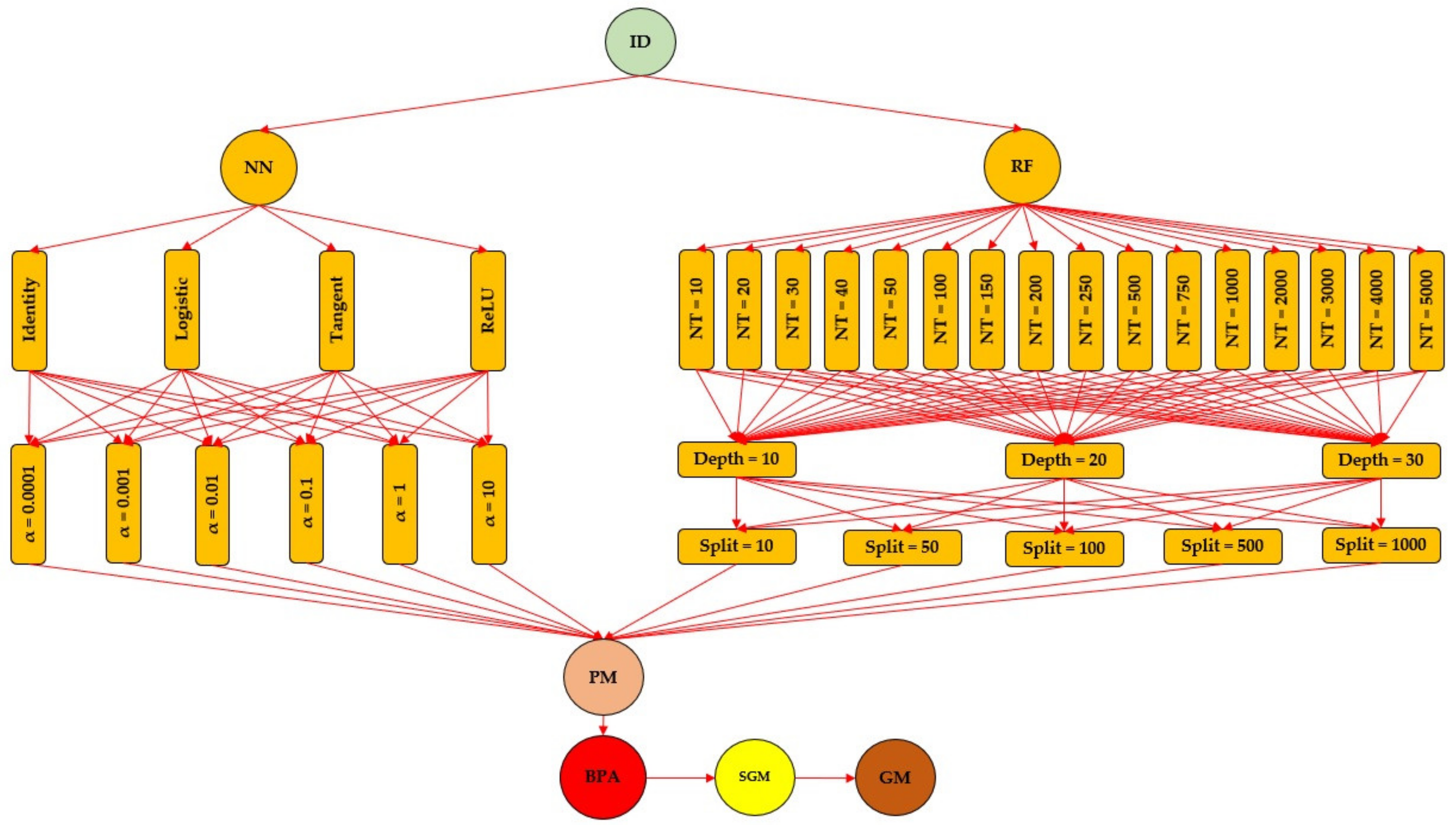
2.3. Machine Learning Algorithms

Two machine learning algorithms were considered, namely the Artificial Neural Networks (hereafter, NN) and Random Forests (hereafter, RF). The choice was based on the popularity of these two machine learning techniques [4,22,23,24,26,30,37] as well as on the capabilities and functionalities of the software used [34] to tune, train and test the models (Section 2.4). By the software used, NN models are implemented in the form of multilayer perceptrons with backpropagation [34,38]. They require tunning of several parameters, many of which were developed so as to increase the computational performance. RF is a machine learning algorithm proposed by Ho [39] and further developed by Breiman [40]. It has the advance of working well on high dimensional data and fast training. Both machine learning algorithms may be used for classification tasks.
Architecture of the NN machine learning algorithms is commonly described by the depth and width, where the depth stands for the number of hidden layers and the width stands for the number of neurons stored in the hidden layers. Recent findings on testing the performance of NNs over acceleration signal data [41] have indicated that developing the architecture towards a maximal one (i.e., increasing the number of neurons and of hidden layers) may contribute to increments in classification performance. In addition, neural nets were found to increase their representational capacity by increasing the number of neurons in them [42]. The maximum depth and width of the NN was used, as enabled by the used software [34], namely the number of hidden layers was set at 3 and the number of neurons was set at 100 per hidden layer. Providing a better chance to learn was also considered by setting the number of iterations to the maximal one enabled by the software [34], that is 1,000,000 iterations. Adam solver (the stochastic gradient descent optimizer) was set and used for all scenarios due to its enhanced performance [43]. Learning process of the NNs is typically controlled by the type of activation (transfer) function used, and by the value set for the regularization parameter. The activation function controls whether or not a neuron will produce an output. The software used for training and testing purposes enables the use of both linear and nonlinear activation functions [34]. In the first category, the software provides the Identity (Linear) activation function (hereafter Identity) whose output is not confined in a given range [44]. In the second category, the software enables the use of Logistic (hereafter Logistic), Hyperbolic Tangent (hereafter Tangent) and Rectified Linear Unit (ReLU, hereafter ReLU) activation functions. Logistic and Tangent activation functions hold output ranges between 0 and 1 and -1 and 1, respectively [44]. ReLU has become the most used activation function due to its high performance [45,46]. For values less than 0 it returns 0 and for values higher than 0, it returns the actual value [44]. All of the above-described functions were considered in the first workflow used to infer the best architecture of the NN model. The second component of the learning process is the regularization parameter, a hyperparameter which controls the shape of decision functions [44]. For the NN machine learning model, and for all the activation functions, the parameter of the regularization term (α) was tuned to take values of 0.0001, 0.001, 0.01, 0.1, 1 and 10 (Figure 2).
Typically, the architecture of the RF algorithm may be controlled at two levels, namely the tree and the forest level. There is a set of hyperparameters that can affect the performance of the model [47]. For instance, the depth of the RF algorithm is characterized by longest path between the root and leaf nodes, and higher depths may contribute to performance enhancement in the training phase but may also overfit the model. If not controlled, the number of splits that can happen in a model may reach to nodes which are completely pure, resulting in tree growth and model overfitting. Number of trees is an important parameter in RF, as more trees would help producing a more generalized result [47]. However, as the number of trees increases, similar to the depth and size of the NNs, the time complexity of the model will increase [47]. In this study, the number of attributes considered at each split was kept at the default value provided by the software, which is the square root of the number of attributes present in the data [48]. The models were trained by controlling two parameters of tree growth, namely the depth, which was set successively at 10, 20 and 30 nodes, and the subset splitting restriction, which was set successively at 10, 50, 100, 500 and 1000 observations (Figure 2). Acknowledging that significant changes in performance could be produced when using smaller numbers of trees, this parameter was varied from 10 to 50 with a step of 10, from 50 to 250 with a step of 50, from 250 to 1000 with a step of 250 and from 1000 to 5000 with a step of 1000 (Figure 2).
In total, 24 (4 activation functions × 6 values set for α) models were trained in the case of NN algorithm, and 240 (6 options for the number of trees × 3 values for the tree depth × 5 values for the split control) models were trained for RF which, together, took a computational time of close to 97 h. In both cases a cross-validation by five folds was used to evaluate the training performance. Evaluation of the best model architecture from each class as well as choosing the best model architecture were mainly based on the overall values of the log loss error function which was the first criterion to differentiate among the 264 models. The minimum values were those indicating the model to choose and, in case of ties, the values of F1 score were used for differentiation (maximum values). When there was a tie also for F1 score, the selection algorithm was repeated at the class level in the order WORK–OFF–SWITCH. Although the log loss error and F1 metric were used for selection, several other performance metrics such as the classification accuracy, precision, recall, and sensitivity were estimated as well (Section 2.4). Once the best architecture was inferred it was used over the training datasets from WF2 (Figure 3). For this purpose, the tuned parameters of the best-performing architecture were kept the same during the tests. Each time, and for each ratio of data in the training and testing datasets, a new model was saved with the purpose of testing it. Additionally, a general model was saved characterizing the inferred best architecture (Figure 2), which was then used to test the invariance of classification performance to systematic data sampling (Figure 4). For this purpose, the general model was tested over the systematically sampled datasets.

2.4. Computer Architecture and Software Used—Performance Evaluation

The tasks of training and testing the machine learning models were performed on a computer architecture that included the following features: system type—Alienware 17 R3, processor—Intel® Core™ i7-6700HQ CPU, 2.60 GHz, 2592 MHz, 4 cores, 8 Logical Processors, installed physical memory (RAM)—16 GB, operating system—Microsoft Windows 10 Home. Microsoft Excel ® (Microsoft, Redmond, WA, USA) was used to store and preprocess the data, including the tasks of dividing data into the necessary subsets, performing simple computations, and of resampling the data. Part of the artwork used in this study was built with the same software. The software used to train and test the machine learning models, as well as to build a part of the artwork, was the Orange Visual Programming Software, version 3.31.1 [34], which holds the necessary functionalities for building and running NN (multi-layer perceptron models with backpropagation) and RF models based on the creation of widget-based workflows. Data, Neural Network, Random Forest, Test and Score, Save Model, Load Model and Predictions widgets were used for training and testing purposes. Based on the multidimensional input data, Scatter Plot widget including its “color regions” and “jittering” graphical features were used to depict the relations between the parameter tuning options and key-selected classification performance metrics for both, NN and RF architectures.
Orange Visual Programming Software enables the computation of several classification performance metrics. The full list of metrics computed for the training and testing phases includes the training and testing time, area under the ROC (receiver operating characteristic, hereafter AUC), classification accuracy (hereafter CA), F1 score, which is the harmonic mean of the classification’s precision and recall (hereafter F1), precision (hereafter PREC), recall (hereafter REC), log loss (cross-entropy) error (hereafter LOG LOSS) and specificity (hereafter SPEC). All of these metrics were computed for all the training and testing tasks and the most important ones were reported where appropriate. For exemplification, however, performance metrics such as the LOG LOSS, F1 score and CA, were compared in more detail in the results section of the paper, including their differences as an effect of the parameters used for tuning (WF1), partition of the data in training and testing subsamples (WF2) and data resampling in the testing subsets (WF3), respectively. For reference, the performance of classifiers is discussed, for instance, in [49]. References on definitions and explanations of the classification performance metrics are given in [50]. Classification accuracy (CA) is one of the important metrics used for evaluating classification models. It is defined as the ratio of correct predictions to the total number of predictions. Recall (REC), or the hit rate [49,50], is defined as the ratio of correctly classified true positives (true positives) to the total number of positives (true positives + false negatives). Precision (PREC) is the ratio of correctly classified positives (true positives) to the total predicted positives (true positives + false positives) [49,50]. F1 score is a metric that balances precision and recall, being better adapted to class imbalance [50]. Orange Visual Programming software computes the LOG LOSS according to the equation given in [51]. Class level and overall ratio values of the performance metrics which characterize the training and testing datasets are typically multiplied by 100 to obtain a percent-based overview of the classification performance [50], an approach that was used in the Results and Discussion section.
In the testing phase, a given model operates over the test data by providing the probability of each instance being classified in a true class. Given the one-dimensionality of the input data, such probabilities were assigned to EN (Euclidian Norm) of the data in the testing datasets to map each instance in a given class (WORK, SWITCH, OFF).

3. Results

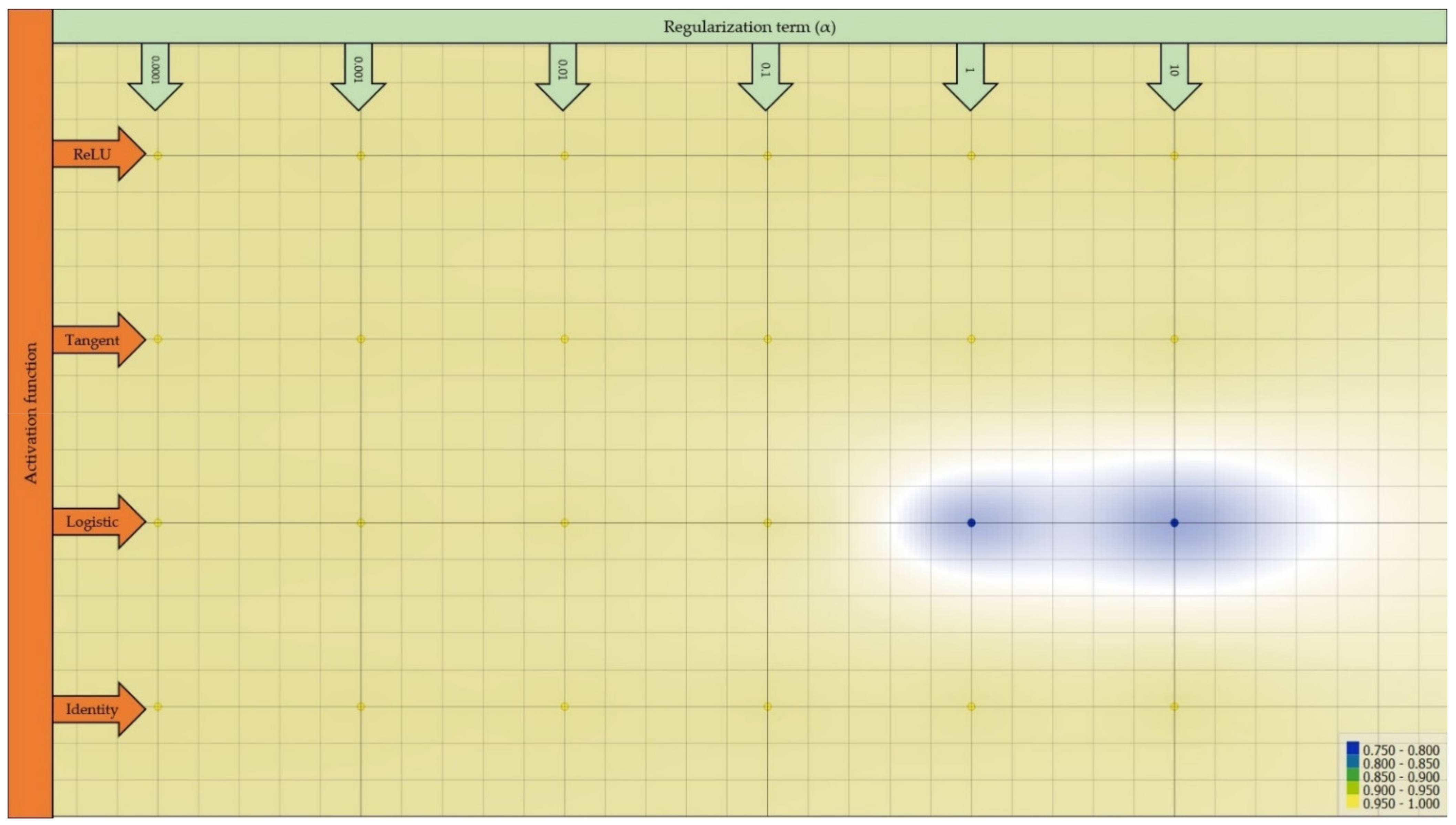
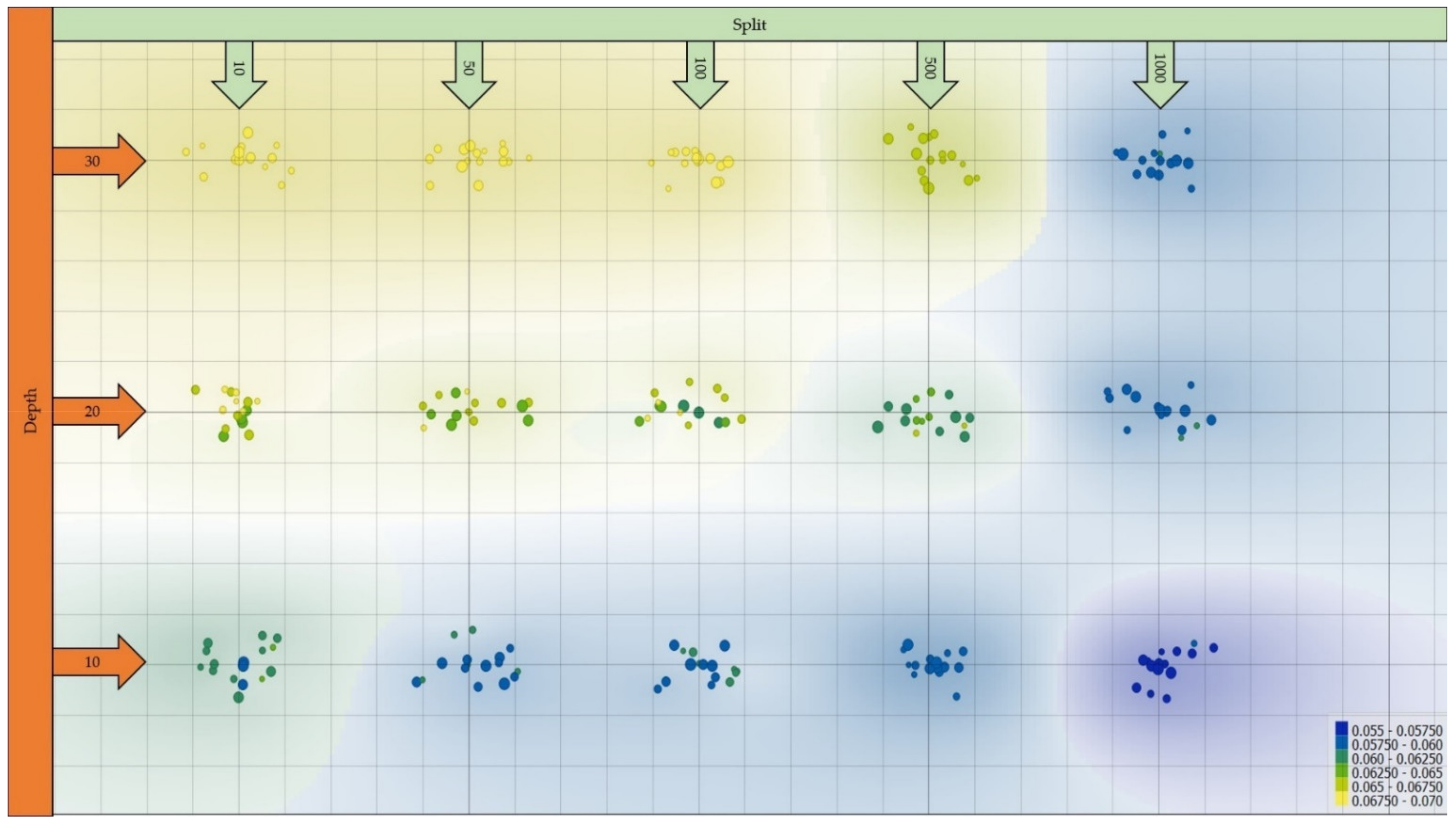
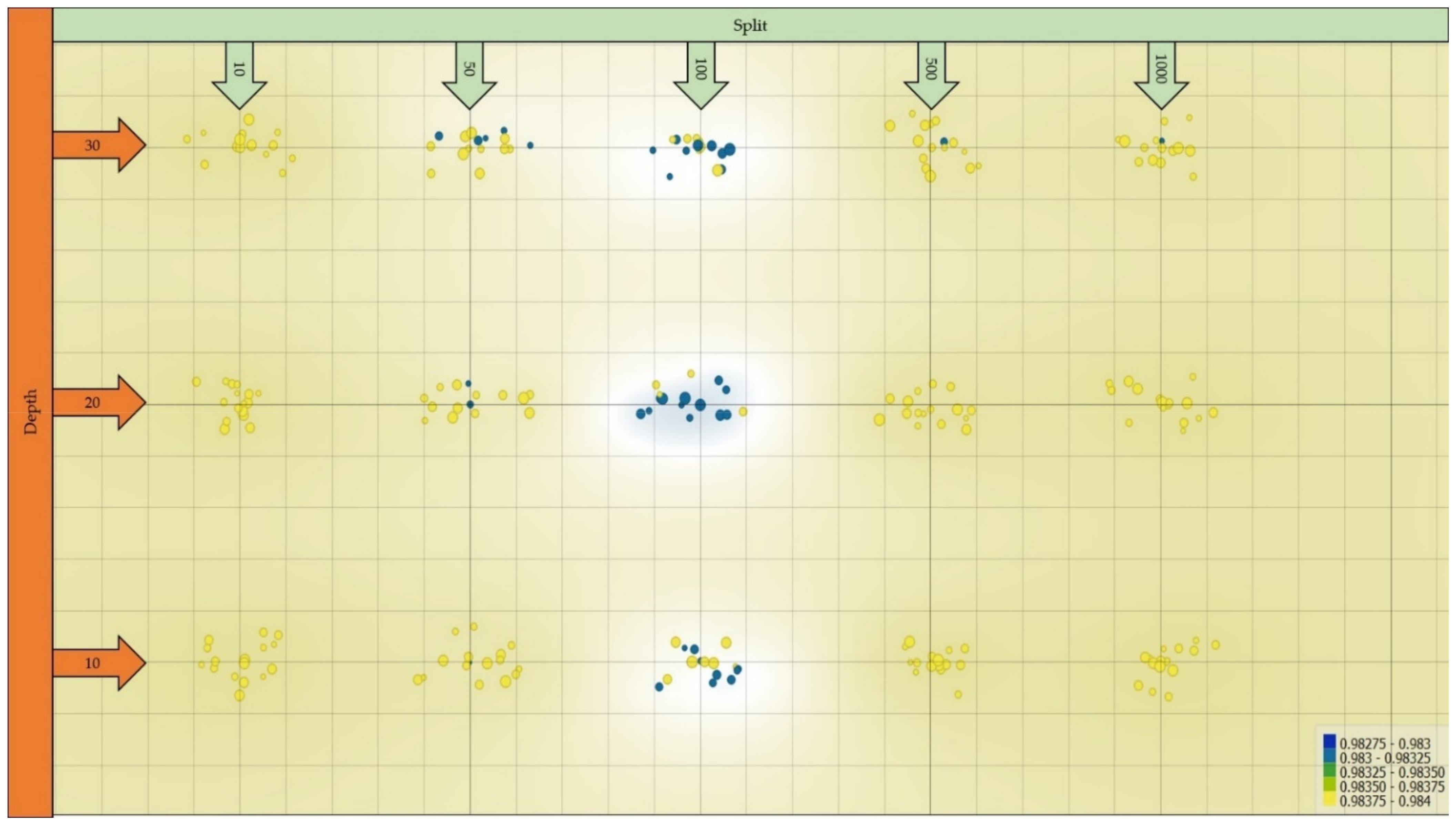
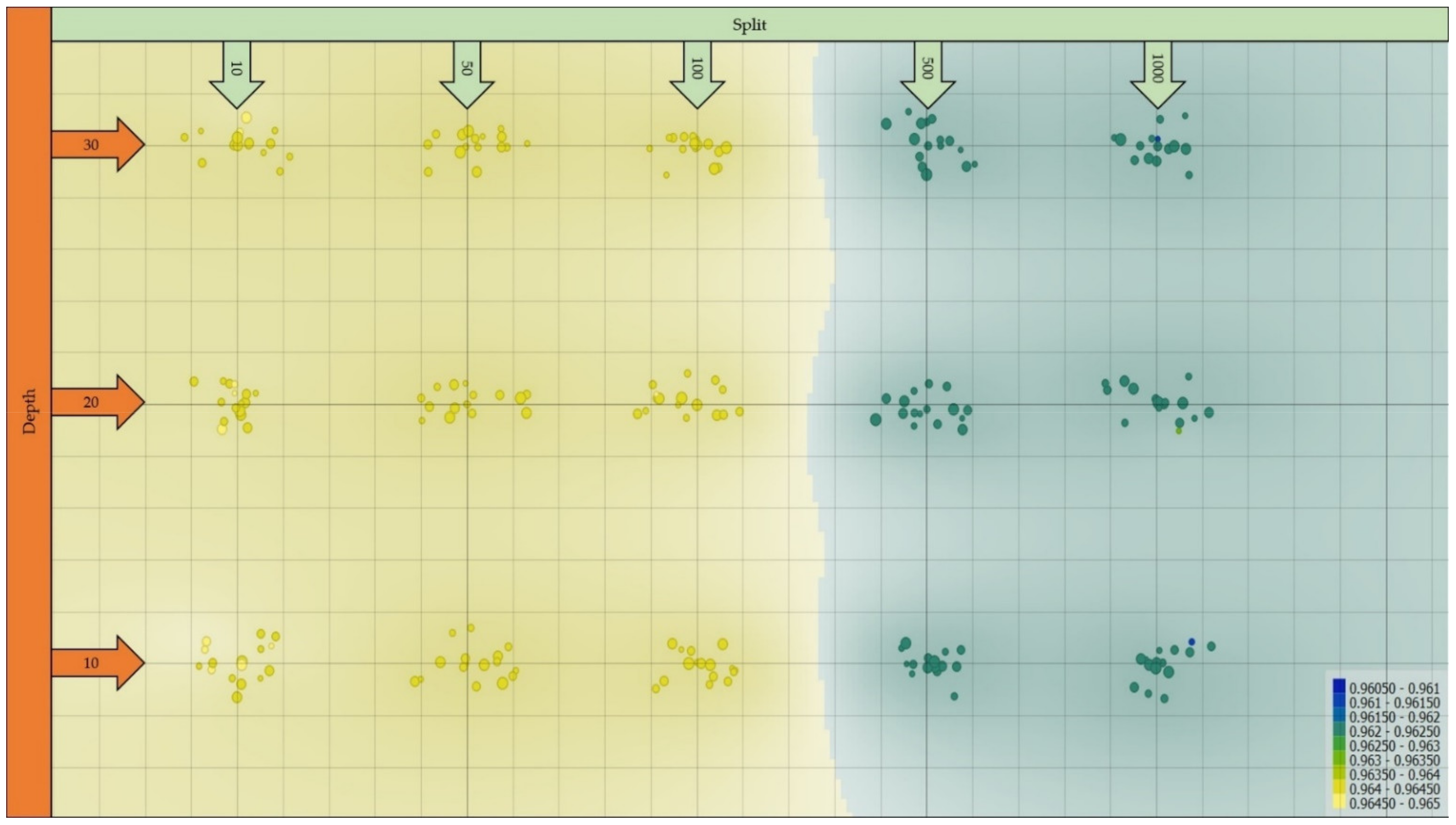
3.1. Best-Performing Model Architecture

The variation of the main classification performance metrics as a function of the models’ architecture is shown in Figure 5, Figure 6, Figure 7, Figure 8 and Figure 9. Figure 5, for instance, plots the LOG LOSS values against the activation functions and regularization terms used in the NN architecture.
There were no major differences in LOG LOSS except those returned by the Logistic activation function when using regularization terms set at 1 and 10 (less complex decision functions). In general, the values of LOG LOSS were in the range of between 5.6 and 6.3% for the 24 trained NN models. Figure 6 shows the variation in F1 score as a function of the models’ architecture, indicating a similar trend. In general, the values of the F1 score varied between 97.9 and 98.4%, indicating a high classification performance of the NN models. A similar data organization is shown in Figure 7, Figure 8 and Figure 9 for the RF model, where each dot stands for a model of a given architecture by jittering the data so as to be visible in the plots. Lower depths (Depth) of the RF model coupled with higher amounts of data preserved at node splitting (Split) were among the highest contributors to lower LOG LOSS errors (Figure 7), which was also generally true for the highest values of the F1 score (Figure 8). In terms of model specificity (Figure 9), there were found two classes, in which highly specific models were generally shaped by lower amounts of data preserved at splits. In general, the LOG LOSS values decreased as a function of the number of trees used to train the models. LOG LOSS and F1 score values varied between 5.8 and 6.9% and 98.3 and 98.4%, respectively. Based on the fixed parameters and criteria described in the Materials and Methods section, the best-performing architecture was identified for a NN machine learning model when using the ReLU activation function and the regularization parameter set at α = 0.01.

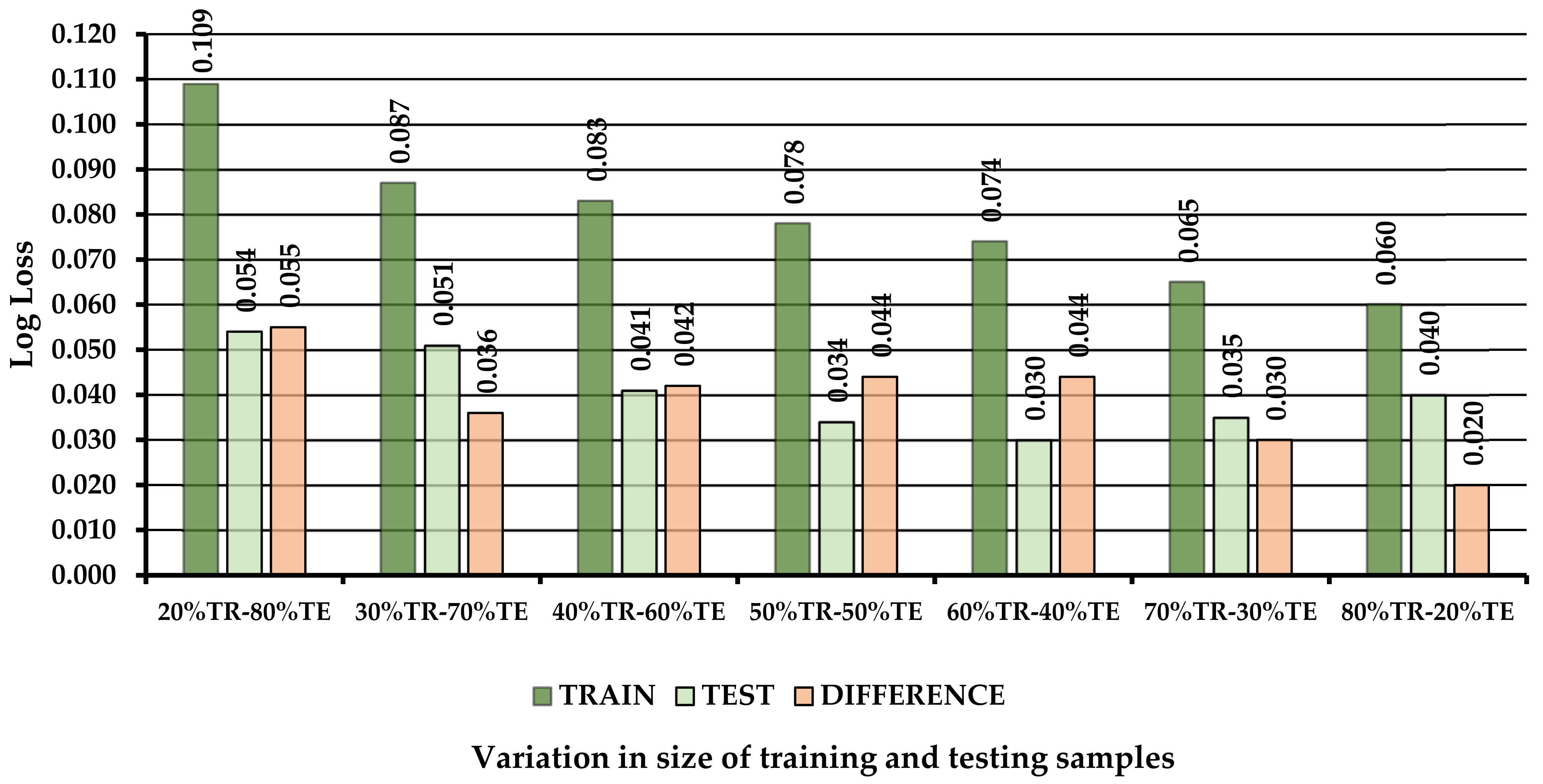
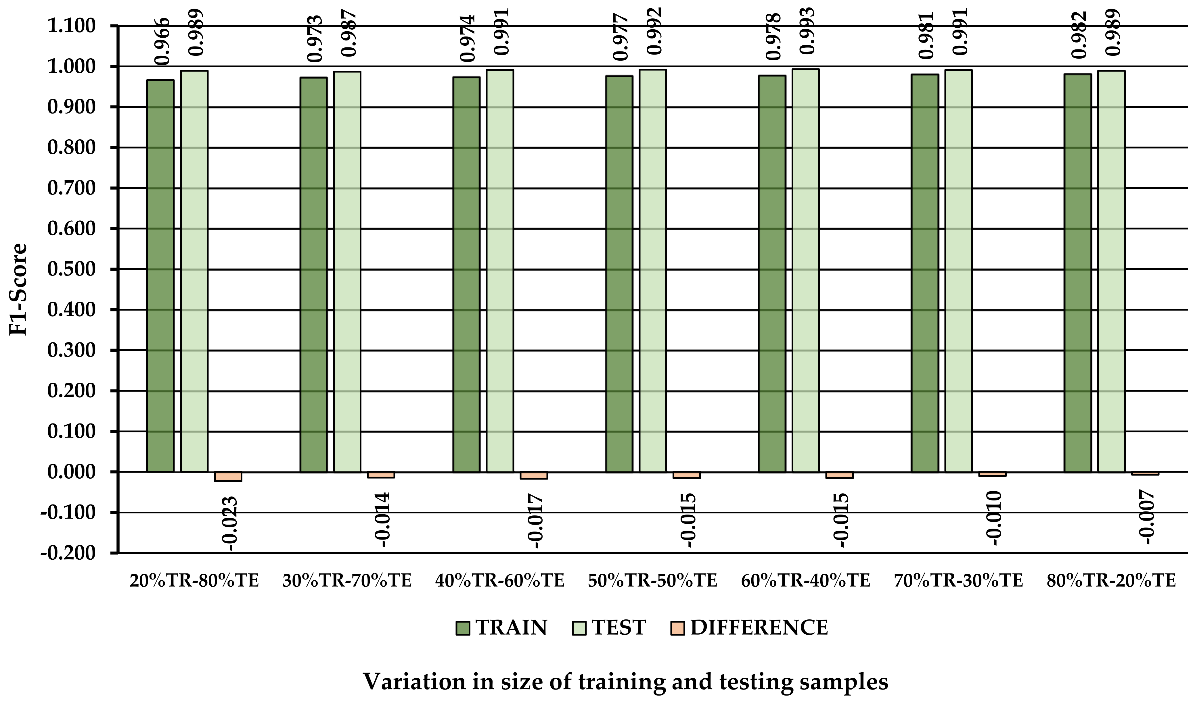
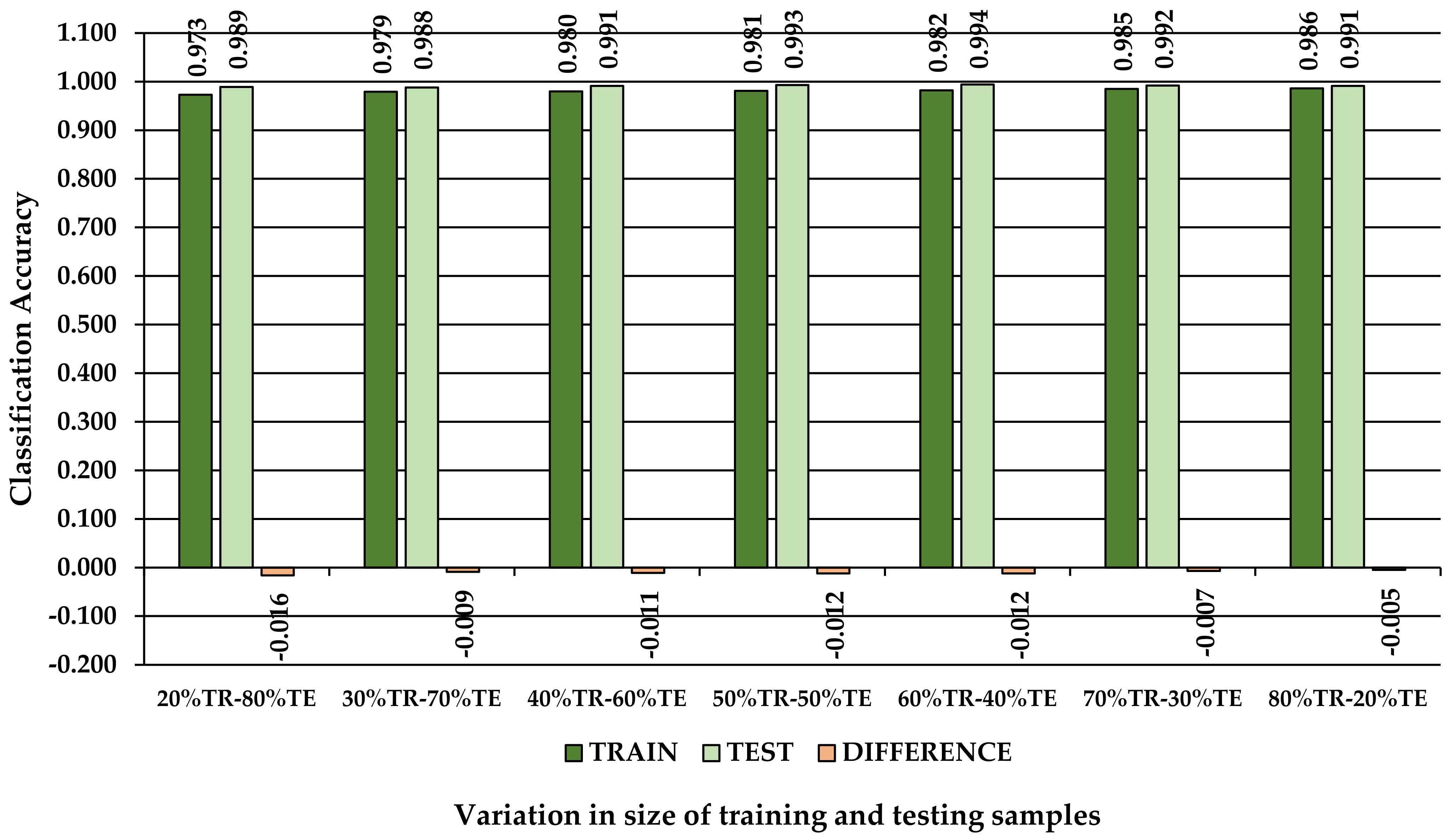
3.2. Effect of Data Share in the Training and Testing Subsets on Classification Performance

The results shown in Figure 10, Figure 11 and Figure 12 and in Table 2 are consistent with the rule of thumb of using a high share of data in the training (TRAIN, TR) as opposed to the testing (TEST, TE) dataset. For instance, Figure 10 shows the variation in LOG LOSS error in the training and testing datasets as well as the absolute differences in values as a function of the share of data used in the subsets divided according to WF2 (Figure 3). A share of 20%–80% has produced the most contrasting results in terms of LOG LOSS error, which was close to 11% in the dataset used for training and close to 6% in the dataset used for testing. However, a model trained on a small data partition (20%) was able to generalize very well on the rest of the data, as proved by the absolute differences between the training and testing values of LOG LOSS error, which was the highest among the tested options (5.4%).
As the share of data used for training increased, the classification error decreased, reaching a value of 6% for a share of 80%–20% in the training and testing datasets in the training phase, respectively (Figure 10). The range of LOG LOSS values also decreased as the amount of data used in the training sample increased. Irrespective of the share of data used for training and testing, the results show that the errors of the testing phase were much lower compared to those of the training phase (Figure 10), ranging from 2 (80%TR-20%TE) to 5.5% (20%TR-80%TE), a fact that proves that the learned models had a high generalization ability. This can be seen also in the variation of F1 (Figure 11) and CA (Figure 12) values which followed a similar trend of improvement as more data were fed into the training sample, with the most important differences occurring up to a data share of 50 to 50%. However, the absolute differences were smaller accounting for 0.7 to 2.3% in the case of F1 score (Figure 11) and for 0.5 to 1.6% in the case of classification accuracy (CA, Figure 12).
Table 2 summarizes the values of the main classification performance metrics computed for the two datasets and data sharing strategy, including the differences found between the values of the metrics.
Precision (PREC) and recall (REC), which are used to compute the F1 score, followed a similar trend in values and in differences as the F1 and CA did. In all, CA, F1, PREC, REC and LOG LOSS, the most important differences were between using a share of 20 to 80%. For the rest of the data partitioning strategies, the differences were much less, typically less than 1% in the case of TRAIN datasets and less than 0.5% in the case of TEST datasets. Altogether, these trends indicate important improvements, sustain the practice rules of data partitioning, show the variance of classification performance as a function of the strategy used for data partitioning and are useful in providing hints for data partitioning attempts.

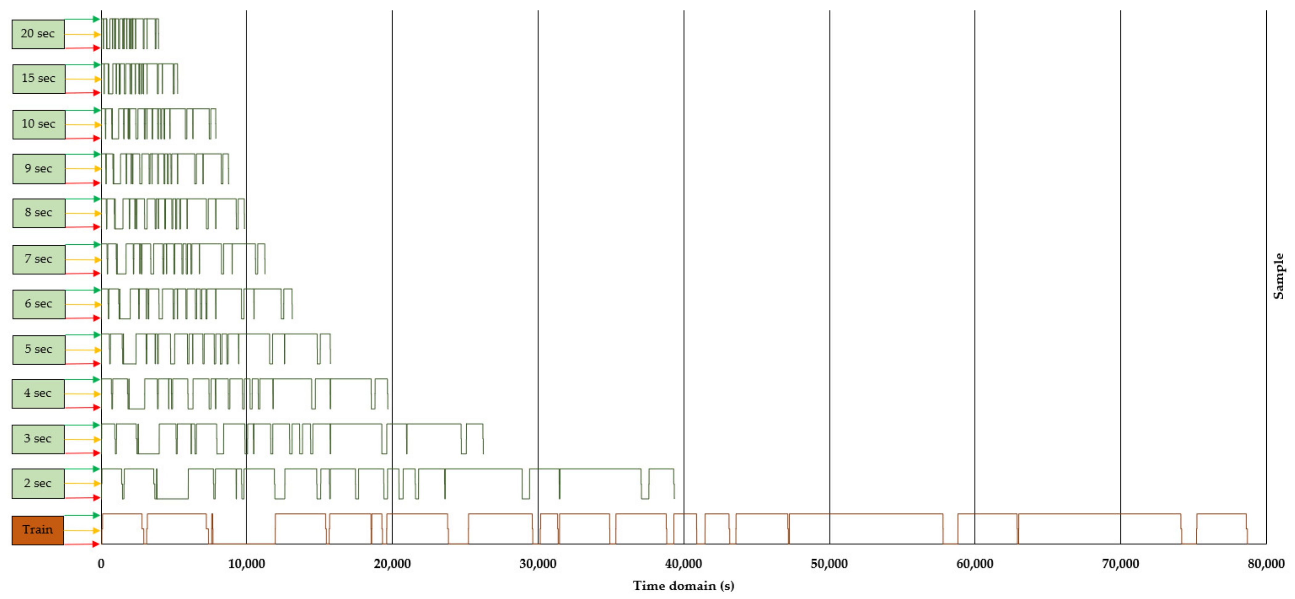
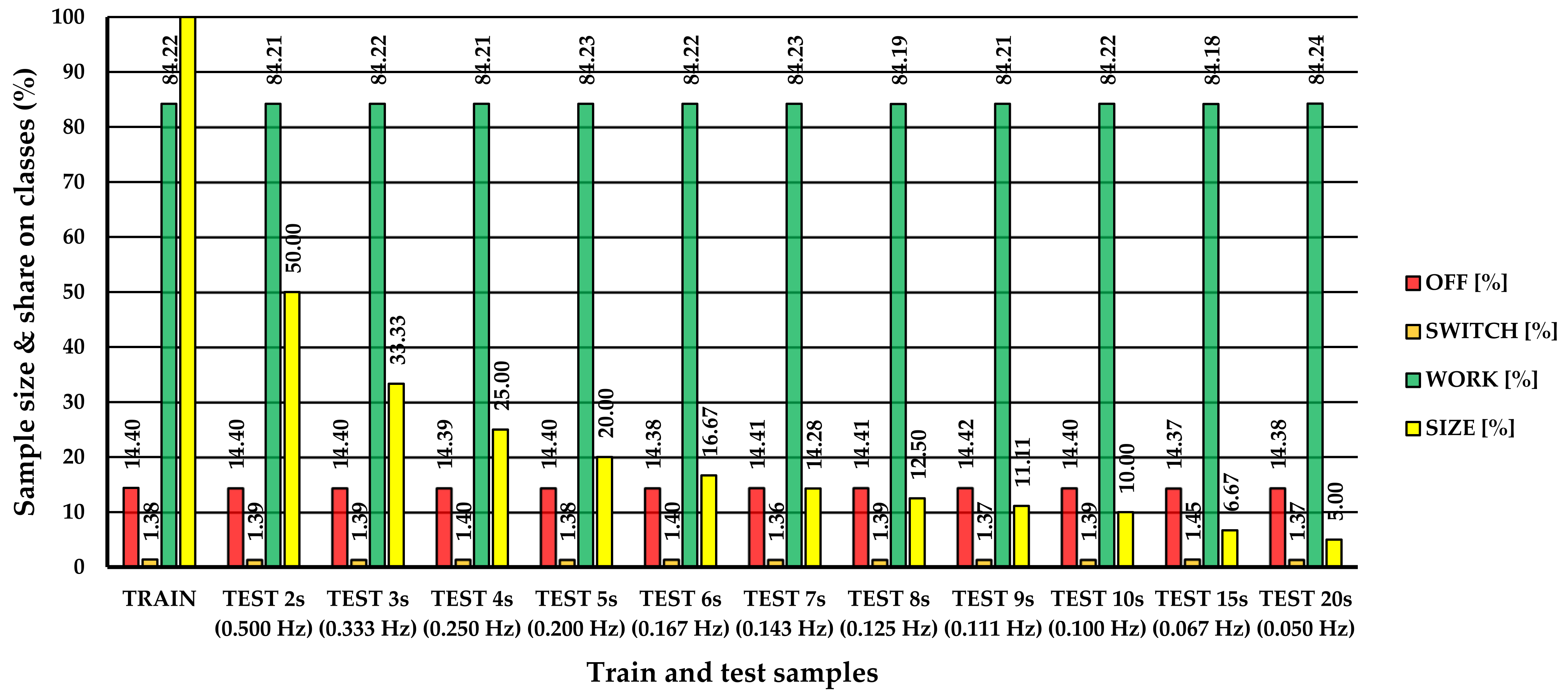
3.3. Effect of Sampling Rate on Classification Performance

By resampling, the original dataset (ID) used to train the general model (WF1, Figure 2) was progressively reduced in size from 78,707 (100%) to 3953 instances (5%). The reduction in size compared to ID is illustrated in Figure 13, which shows the 11 newly created testing datasets (WF3, Figure 4) plotted in the time domain. Figure 14, on the other hand, shows the size of the systematically sampled datasets relative to the original dataset (ID).
For example, by systematically resampling ID at 15 and 20 s, respectively, the amount of data in the testing sets was reduced to less than 7%. However, the used sampling procedure has preserved the share of data on true classes which differed between the original (ID) and sampled datasets by less than 0.1% in all classes. Therefore, a relative data share of ca. 14%–1%–85% was preserved in all datasets for the OFF, SWITCH and WORK classes, respectively.
The results summarized in Table 3 prove the invariance of classification performance metrics of the testing phase to the amount of data used in the testing datasets. Differences brought by the testing sample size in LOG LOSS error are illustrated in Figure 15. Although they were both positive and negative, they were only minor, accounting for a maximum absolute value of 0.2%. Figure 16 and Figure 17 indicate similar trends of differences in F1 score and classification accuracy, which did not exceed an absolute value of 0.2%. As observed (Table 3, Figure 15, Figure 16 and Figure 17), there were no evident increasing or decreasing trends in the differences between LOG LOSS, F1 and CA as a function of the sampling rate used, although higher differences were found for F1 and CA in the TEST 20 s data subset as compared to the initial dataset (ID, TRAIN).
These results illustrate well the invariance of the general model in terms of classification performance when performing on newly generated datasets, although they were artificially created. In particular, the differences in terms of LOG LOSS, F1 and CA were minor, accounting for up to 0.2% for that case in which the data sample used for testing was the smallest one. Taking as a reference the general model built by the WF1, it correctly classified close to 99% of the data. The F1 score which balances the precision (PREC) and recall (REC) also indicated a high performance, accounting for 98.4%, while LOGLOSS was 5.6%. With minor differences (up to 0.2%) this classification performance was preserved in all of the testing models.

4. Discussion

Several studies have tested the capability of NN models in correctly predicting class-based outcomes with various applications in forestry, some of which have focused on using acceleration signals to make predictions by machine learning [4,24,52]. Most of them agree that general classification accuracies of up to 100% may be achieved depending on several factors such as the complexity of classification, signal quality and accuracy of data labeling. In contrast, some have opted for using RF machine learning algorithms for classification purposes [23,26], finding also highly accurate classifications when collecting data multimodally. Unless a given device holds the capabilities and can be used to collect data multimodally by integrating several sensors, the procurement of separate devices would incur more costs, limiting the economic efficiency of data collection. Nevertheless, by the use of a multimodal approach and RF algorithms, the classification outcomes were found to be similar to those provided by NN, with values of between 97.7 and 99.6% [23,26]. Therefore, it is obvious that when several machine learning algorithms enable classification over a given signal typology, several options need to be checked to evaluate their performance.
With some minor exceptions in regard to the activation function used for NN and the amount of data preserved at a node and the depth of the trees, the classification performance measured by the LOG LOSS error, F1 score and classification accuracy did not vary widely and returned no evident contrasts as an effect of the machine learning architectures used. Therefore, the best model architecture was selected using the first criterion, namely the error during training which was found to be the lowest for an NN architecture when using the ReLU activation function and α set at 0.01. It turns out that the best-performing models reported in other studies checking the effect of classification performance on acceleration data had similar architectures, placing the use of the ReLU activation function and of the regularization terms of up to 0.1 among the best options in terms of classification performance [24,52]. However, the performance of NN depends also on several other factors [53,54], including signal quality and other issues specific to classification tasks such as intra-class variability and inter-class similarity. Altogether, the classification performance of the selected architecture was very high, with a classification accuracy of 98.7%, an F1 score of 98.4%, a precision of 98.4% a recall of 98.7% and an error of 5.6%. Transition parts in the acceleration signal (SWITCH) were poorly classified compared to OFF (CA = 99.4%, F1 = 98.0%, PREC = 99.4%, REC = 99.4%, LOG LOSS = 2.2%) and WORK (CA = 99.3%, F1 = 99.6%, PREC = 99.2%, REC = 99.9%, LOG LOSS = 3.6%) events, although their classification error was still low (LOG LOSS = 5.2%). In addition, there was an evident class imbalance with a relative data share of ca. 14%–1%–85% for OFF, SWITCH and WORK events, respectively. This may raise the question of how the developed model would perform in cases in which the data collection will be deployed for longer periods of time. In this regard, it is likely that the share of SWITCH events will decrease in the data samples, mainly at the expense of increasing the share of OFF events since the data loggers would also need to operate during the night, at weekends and during legal holidays. As such, the two classes characterized by the highest performance will dominate the data, potentially making the model more effective in classification. In relation to the SWITCH events which were poorly classified, previous studies have already described how the inter-class similarity, which was typical to this event, may affect the classification performance [4,24,52].
The general rule of using most of the data in the training phase held true. However, the differences in performance were not particularly contrasting in relation to the share of data used in the training and testing subsets, although the LOG LOSS error in the training dataset decreased as it contained more data. Along with improved values of the F1 score and of the classification accuracy as more data were added to the training data subset, this indicates that a model trained over all data would hold better predictive capabilities. What is to be emphasized is that the generalization ability (testing phase) measured by the value of the LOG LOSS error, F1 score and classification accuracy was improved. Accordingly, the LOG LOSS was lower in the testing phase from 2 to 5.5%, while the F1 score and classification accuracy were higher in the testing phase from 0.7 to 2.3 and 0.5 to 1.6%, respectively. All of these results are coming in high contrast to those of the previous studies which have found either similar [4] or higher values of classification errors and lower values in terms of classification accuracy in the testing phase [24,52].
The battery life of a data logger such as that used herein is assumed to be ca. 1000 h while its internal memory (4 MB) can hold 168,042 readings made in the normal data collection mode [55]. More or less this means that, in theory, one can cover close to two days of observation at a sampling rate of 1 s (1 Hz) before downloading the data. However, the data collection time frame can be effectively managed by assuming that a higher sampling rate would still accurately reflect the operational pattern in the collected data. By their functional construction, machines such as that described herein may be characterized by relatively long events of working intercalated by short events of switching and long events of being off. With the capabilities of the data logger in mind, a sampling rate of 2 s would double data collection capabilities, while sampling rates of 10 and 20 s would extend the data collection period by ca. 5 to 20 times, meaning that sampling at 20 s would cover a timeframe of more than one month. Therefore, increasing the value of the sampling rate will only prolong further the memory and battery availability. In this regard, by systematically sampling the initial dataset at rates of 2 to 20 s, the share of classes was preserved. Moreover, the general model performed better and similarly in the testing phase, irrespective of the testing dataset used, which is an indication that further data sampled at different rates may be fed into the model which would be able to output a high classification performance. Overall, the generalization errors were improved in the testing phases by up to 0.2% and only in three cases did the testing phase yield higher values of the LOG LOSS. Similar patterns were found in the F1 score and classification accuracies which were generally either the same or higher in values at the testing phase.
As in any other studies on the topic, there are some limitations to be addressed. A first limitation is that of collecting the acceleration data by considering only coniferous logs. As known, a given acceleration signal contains three important components: movement, gravity and noise [56]. Therefore, in the case of processing hardwoods, it is likely to obtain a more differentiated (higher) response in the magnitude of acceleration during the WORK events as the interaction between the logs and blades will produce more vibration. If this does occur, the performance of the model could be an issue that may need additional checking. However, the NN tools of the software used perform by default a normalization procedure over the data before feeding it to the model [57], a fact that serves in weighting the importance of high magnitude data and still preserving the relationships between the original data [58,59]. The same may apply to the variance in log dimensions, particularly to their diameters by reducing or increasing the contact area between the blades and logs which, in theory, would decrease or increase the amount of vibration. On the opposite side, a validation of the model would be required by feeding it with long-term collected, unseen data. In this regard, and based on the performance of the selected machine learning architecture, it is likely to obtain a high classification performance in such a validation phase. Once proved to have a high performance on new datasets, the rest of the steps required to automatically extract and systematize the data, as well as those required for prediction, could be easily managed by the software components described in the Material and Methods section.
Last but not least, the applicability of the described methods may be extended to other sawmilling machines assuming a similar operational pattern in the time domain. This is because, by their construction, they produce vibration during working events. However, the quality of the milled lumber has become of great concern lately [60] and this will possibly become a driver of technological change. Until such changes occur, the proposed model could solve the problems of long-term operational monitoring while after that it could serve, by adaptation, in monitoring operations when such capabilities are not embodied in the sawmilling equipment.

5. Conclusions

Monitoring the operational performance of sawmilling facilities is important for both science and practice. Accordingly, the tools used to obtain useful information need to be adapted to extend data collection and inference capabilities. A robust machine learning model was developed with the purpose of using it to infer the operational events based on lower sampling rates, so as to be able to extend data collection capabilities by low-cost acceleration sensors.
The results indicate a high performance of the model which was less sensitive to the amount of data used to train it, although some variation was found. In this regard, neural networks performed better than random forest algorithms in terms of classification performance. Indeed, they needed more training time, but at this point, this cannot be seen as a limitation since the model is readily available for feeding with new data. The developed model not only preserves a high classification performance in the training and testing phases but it also seems to be invariant to lower sampling rates, making it useful for prediction over long-term collected data. These model properties indicate a high degree of stability to the data potentially fed to the model, as well as a capability enhancement in the sense of lowering the sampling rate of the data to be fed into it.
Altogether, the proposed approach is promising in enabling the use of cheap data collectors to be operated for extended periods in various locations and has the capability of saving human resources and money associated with data collection. Further tests would be required to validate the model, which could be straightforward given the relatively high differentiation which was found at the class level, enabling a visual judgment of predicted classes.

Author Contributions

Conceptualization, S.A.B. and A.R.P.; Data curation, S.A.B., G.O.F. and O.O.-S.; Formal analysis, S.A.B., G.O.F. and O.O.-S.; Investigation, G.O.F. and O.O.-S.; Methodology, S.A.B. and A.R.P.; Project administration, S.A.B. and A.R.P.; Resources, S.A.B., G.O.F. and A.R.P.; Software, S.A.B.; Supervision, S.A.B. and A.R.P.; Visualization, S.A.B.; Writing—original draft, S.A.B., G.O.F. and A.R.P.; Writing—review and editing, S.A.B. and A.R.P. All authors have read and agreed to the published version of the manuscript.

Funding

Some activities of this work were funded by the inter-institutional agreement between the Transilvania University of Braşov (Romania) and the Mediterranean University of Reggio Calabria (Italy).

Data Availability Statement

Data supporting this study may be provided upon reasonable request to the first author of the study.

Acknowledgments

The authors would like to thank the Department of Forest Engineering, Forest Management Planning and Terrestrial Measurements, Faculty of Silviculture and Forest Engineering, Transilvania University of Brasov, for providing the equipment needed to carry on this work. The authors would like to thank the company which supported this research and which wished to remain anonymous.

Conflicts of Interest

The authors declare no conflict of interest.

References

  1. Shahi, S.K.; Dia, M.; Yan, P.; Choudhury, S. Developing and training artificial neural networks using bootstrap data envelopment analysis for best performance modeling of sawmills in Ontario. J. Model. Manag. 2022, 17, 788–811. [Google Scholar] [CrossRef]
  2. Schreiner, F.; Thorenz, B.; Schmidt, J.; Friedrich, M.; Döpper, F. Development of a measuring and control unit for an intelligent adjustment of process parameters in sawing. MM Sci. J. 2021, 5, 5203–5210. [Google Scholar] [CrossRef]
  3. Borz, S.A.; Oghnoum, M.; Marcu, M.V.; Lorincz, A.; Proto, A.R. Performance of small-scale sawmilling operations: A case study on time consumption, productivity and main ergonomics for a manually-driven bandsaw. Forests 2021, 12, 810. [Google Scholar] [CrossRef]
  4. Cheța, M.; Marcu, M.V.; Iordache, E.; Borz, S.A. Testing the capability of low-cost tools and artificial intelligence techniques to automatically detect operations done by a small-sized manually driven bandsaw. Forests 2020, 11, 739. [Google Scholar] [CrossRef]
  5. Cedamon, E.D.; Harrison, S.; Herbohn, J. Comparative analysis of on-site free-hand chainsaw milling and fixed site mini-bandsaw milling of smallholder timber. Small Scale For. 2013, 12, 389–401. [Google Scholar] [CrossRef]
  6. De Lasaux, M.J.; Spinelli, R.; Hartsough, B.R.; Magagnotti, N. Using a small-log mobile sawmill system to contain fuel reduction treatment cost on small parcels. Small Scale For. 2009, 8, 367–379. [Google Scholar] [CrossRef]
  7. Gigoraş, D.; Borz, S.A. Factors affecting the effective time consumption, wood recovery rate and feeding speed when manufacturing lumber using a FBO-02 CUT mobile bandsaw. Wood Res. 2015, 60, 329–338. [Google Scholar]
  8. Venn, T.J.; McGavin, R.L.; Leggate, W.W. Costs of portable sawmilling timbers from the acacia woodlands of Western Queensland, Australia. Small Scale For. Econ. Manag. Policy 2004, 3, 161–175. [Google Scholar] [CrossRef]
  9. Telford, C.G. Small Sawmill Operator’s Manual. Agriculture Handbook No 27—January 1952; United States Department of Agriculture: Washington, DC, USA, 1952. [Google Scholar]
  10. FAO. Small and Medium Sawmills in Developing Countries; Forestry Paper No. 28; FAO: Rome, Italy, 1981. [Google Scholar]
  11. Grönlund, A. Sågverksteknik del 2—Processen; Sveriges Skogsindustriförbund: Markaryd, Sweden, 1992; p. 270. [Google Scholar]
  12. Lundahl, C.G. Optimized Processes in Sawmills. Licentiate Thesis, Luleå University of Technology, Skellefteå, Sweden, 2007. [Google Scholar]
  13. Hyytiäinen, A.; Viitanen, J.; Mutanen, A. Production efficiency of independent Finnish sawmills in the 2000’s. Balt. For. 2011, 17, 280–287. [Google Scholar]
  14. Spinelli, R.; Visser, R.; Magagnotti, N.; Lombardini, C.; Ottaviani, G. The effect of partial automation on the productivity and cost of a mobile tower yarder. Ann. For. Res. 2020, 63, 3–14. [Google Scholar] [CrossRef]
  15. Borz, S.A. Turning a winch skidder into a self-data collection machine using external sensors: A methodological concept. Bull. Transilv. Univ. Braşov 2016, 9, 1–6. [Google Scholar]
  16. Cheța, M.; Borz, S.A. Automating data extraction from GPS files and sound pressure level sensors with application in cable yarding time and motion studies. Bull. Transilv. Univ. Braşov 2017, 10, 1–10. [Google Scholar]
  17. Björheden, R.; Apel, K.; Shiba, M.; Thompson, M. IUFRO Forest Work Study Nomenclature; Swedish University of Agricultural Science, Department of Operational Efficiency: Grapenberg, Sweden, 1995. [Google Scholar]
  18. Acuna, M.; Bigot, M.; Guerra, S.; Hartsough, B.; Kanzian, C.; Kärhä, K.; Lindroos, O.; Magagnotti, N.; Roux, S.; Spinelli, R.; et al. Good Practice Guidelines for Biomass Production Studies; Magagnotti, N., Spinelli, R., Eds.; CNR IVALSA: Sesto Fiorentino, Italy, 2012; Available online: http://www.forestenergy.org/pages/cost-action-fp0902/good-practice-guidelines/ (accessed on 15 April 2018).
  19. Ištvanić, J.; Lučić, R.B.; Jug, M.; Karan, R. Analysis of factors affecting log band saw capacity. Croat. J. For. Eng. 2009, 30, 27–35. [Google Scholar]
  20. Muşat, E.C.; Apăfăian, A.I.; Ignea, G.; Ciobanu, V.D.; Iordache, E.; Derczeni, R.A.; Spârchez, G.; Vasilescu, M.M.; Borz, S.A. Time expenditure in computer aided time studies implemented for highly mechanized forest equipment. Ann. For. Res. 2016, 59, 129–144. [Google Scholar] [CrossRef]
  21. Spinelli, R.; Laina-Relano, R.; Magagnotti, N.; Tolosana, E. Determining observer effect and method effects on the accuracy of elemental time studies in forest operations. Balt. For. 2013, 19, 301–306. [Google Scholar]
  22. Borz, S.A.; Păun, M. Integrating offline object tracking, signal processing, and artificial intelligence to classify relevant events in sawmilling operations. Forests 2020, 11, 1333. [Google Scholar] [CrossRef]
  23. Becker, R.M.; Keefe, R.F. A novel smartphone-based activity recognition modelling method for tracked equipment in forest operations. PLoS ONE 2022, 17, e0266568. [Google Scholar] [CrossRef]
  24. Borz, S.A. Development of a modality-invariant multi-layer perceptron to predict operational events in motor-manual willow felling operations. Forests 2021, 12, 406. [Google Scholar] [CrossRef]
  25. Borz, S.A.; Talagai, N.; Cheţa, M.; Chiriloiu, D.; Gavilanes Montoya, A.V.; Castillo Vizuete, D.D.; Marcu, M.V. Physical strain, exposure to noise and postural assessment in motor-manual felling of willow short rotation coppice: Results of a preliminary study. Croat. J. Eng. 2019, 40, 377–388. [Google Scholar] [CrossRef]
  26. Keefe, R.F.; Zimbelman, E.G.; Wempe, A.M. Use of smartphone sensors to quantify the productive cycle elements of hand fallers on industrial cable logging operations. Int. J. For. Eng. 2019, 30, 132–143. [Google Scholar] [CrossRef]
  27. Marogel-Popa, T.; Cheța, M.; Marcu, M.V.; Duță, C.I.; Ioraș, F.; Borz, S.A. Manual cultivation operations in poplar stands: A characterization of job difficulty and risks of health impairment. Int. J. Environ. Res. Public Health 2019, 16, 1911. [Google Scholar] [CrossRef] [PubMed] [Green Version]
  28. McDonald, T.P.; Fulton, J.P.; Darr, M.J.; Gallagher, T.V. Evaluation of a system to spatially monitor hand planting of pine seedlings. Comput. Electron. Agric. 2008, 64, 173–182. [Google Scholar] [CrossRef]
  29. Strandgard, M.; Mitchell, R. Automated time study of forwarders using GPS and a vibration sensor. Croat. J. Eng. 2015, 36, 175–184. [Google Scholar]
  30. Muşat, E.C.; Borz, S.A. Learning from acceleration data to differentiate the posture, dynamic and static work of the back: An experimental setup. Healthcare 2022, 10, 916. [Google Scholar] [CrossRef]
  31. Picchio, R.; Proto, A.R.; Civitarese, V.; Di Marzio, N.; Latterini, F. Recent contributions of some fields of the electronics in development of forest operations technologies. Electronics 2019, 8, 1465. [Google Scholar] [CrossRef] [Green Version]
  32. Wescoat, E.; Krugh, M.; Henderson, A.; Goodnough, J.; Mears, L. Vibration analysis using unsupervised learning. Procedia Manuf. 2019, 34, 876–888. [Google Scholar] [CrossRef]
  33. Borz, S.A.; Talagai, N.; Cheţa, M.; Gavilanes Montoya, A.V.; Castillo Vizuete, D.D. Automating data collection in motor-manual time and motion studies implemented in a willow short rotation coppice. Bioresources 2018, 13, 3236–3249. [Google Scholar] [CrossRef]
  34. Demsar, J.; Curk, T.; Erjavec, A.; Gorup, C.; Hocevar, T.; Milutinovic, M.; Mozina, M.; Polajnar, M.; Toplak, M.; Staric, A.; et al. Orange: Data Mining Toolbox in Python. J. Mach. Learn. Res. 2013, 14, 2349–2353. [Google Scholar]
  35. R Interface to Keras. Available online: https://keras.rstudio.com/ (accessed on 19 May 2022).
  36. Smith, S.W. Digital Signal Processing—A Practical Guide for Engineers and Scientists, 1st ed.; Newnes—Elsevier Science: Burlington, MA, USA, 2003. [Google Scholar]
  37. Proto, A.R.; Sperandio, G.; Costa, C.; Maesano, M.; Antonucci, F.; Macri, G.; Scarascia Mugnozza, G.; Zimbalatti, G. A three-step neural network artificial intelligence modeling approach for time, productivity and costs prediction: A case study in Italian forestry. Croat. J. For. Eng. 2020, 41, 15. [Google Scholar] [CrossRef]
  38. Neural Network Models (Supervised). Multi-Layer Perceptron. Available online: https://scikit-learn.org/stable/modules/neural_networks_supervised.html (accessed on 19 May 2022).
  39. Ho, T.K. Random decision forests. In Proceedings of the 3rd International Conference on Document Analysis and Recognition, Montreal, QC, Canada, 14–16 August 1995; pp. 278–282. [Google Scholar]
  40. Breiman, L. Random forests. Mach. Learn. 2001, 45, 5–32. [Google Scholar] [CrossRef] [Green Version]
  41. Cheța, M.; Marcu, M.V.; Borz, S.A. Effect of training parameters on the ability of artificial neural networks to learn: A simulation on accelerometer data for task recognition in motor-manual felling and processing. BUT Ser. II For. Wood Ind. Agric. Food Eng. 2020, 13, 19–36. [Google Scholar] [CrossRef]
  42. Goodfellow, J.; Bengio, Y.; Courville, A. Deep Learning; MIT Press: Cambridge, MA, USA, 2016; Available online: https://www.deeplearningbook.org/ (accessed on 19 May 2022).
  43. Kingma, D.P.; Ba, J.L. 2015: ADAM: A method for stochastic optimization. In Proceedings of the 3rd International Conference on Learning Representations (ICLR 2015), San Diego, CA, USA, 7–9 May 2015. [Google Scholar]
  44. Activation Functions in Neural Networks. Available online: https://towardsdatascience.com/activation-functions-neural-networks-1cbd9f8d91d6 (accessed on 19 May 2022).
  45. Maas, A.L.; Hannun, A.Y.; Ng, A.Y. Rectifier nonlinearities improve neural network acoustic models. In Proceedings of the 30th International Conference on Machine Learning (ICML 2013), Atlanta, GA, USA, 16–21 June 2013. [Google Scholar]
  46. Nair, V.; Hinton, G.E. Rectified linear units improve restricted Boltzmann machines. In Proceedings of the 27th International Conference on Machine Learning (ICML 2010), Haifa, Israel, 21–24 June 2010. [Google Scholar]
  47. A Beginner’s Guide to Random Forest Hyperparameter Tunning. Available online: https://www.analyticsvidhya.com/blog/2020/03/beginners-guide-random-forest-hyperparameter-tuning/?utm_source=blog&utm_medium=decision-tree-vs-random-forest-algorithm (accessed on 19 May 2022).
  48. Orange Visual Programming. Random Forest. Available online: https://orange3.readthedocs.io/projects/orange-visual-programming/en/latest/widgets/model/randomforest.html (accessed on 19 May 2022).
  49. Fawcett, T. An introduction to ROC analysis. Pattern Recogn. Lett. 2006, 27, 861–874. [Google Scholar] [CrossRef]
  50. Kamilaris, A.; Prenafeta-Boldu, F.X. Deep learning in agriculture: A survey. Comput. Electron. Agric. 2018, 147, 70–90. [Google Scholar] [CrossRef] [Green Version]
  51. Sklearn Metrics. Log Loss. Available online: https://scikit-learn.org/stable/modules/generated/sklearn.metrics.log_loss.html (accessed on 19 May 2022).
  52. Castro Pérez, S.N.; Borz, S.A. Improving the event-based classification accuracy in pit-drilling operations: An application by neural networks and median filtering of the acceleration input data. Sensors 2021, 21, 6288. [Google Scholar] [CrossRef]
  53. Chen, K.; Zhang, D.; Yao, L.; Guo, B.; Yu, Z.; Liu, Y. Deep learning for sensor-based human activity recognition: Overview, challenges and opportunities. J. ACM 2018, 37, 111. [Google Scholar] [CrossRef]
  54. Bulling, A.; Blanke, U.; Schiele, B. A tutorial of human activity recognition using body-worn inertial sensors. ACM Comput. Surv. 2014, 46, 33. [Google Scholar] [CrossRef]
  55. Extech® User Manual. 3-Axis G-Force Datalogger. Model VB300. Available online: http://www.extech.com/products/resources/VB300_UM-en.pdf (accessed on 19 May 2022).
  56. van Hees, V.T.; Gorzelniak, L.; León, E.C.D.; Eder, M.; Pias, M.; Taherian, S.; Ekelund, U.; Renström, F.; Franks, P.W.; Horsch, A.; et al. Separating movement and gravity components in an acceleration signal and implications for the assessment of human daily physical activity. PLoS ONE 2013, 8, e61691. [Google Scholar] [CrossRef] [Green Version]
  57. Orange Visual Programming. Neural Network. Available online: https://orange3.readthedocs.io/projects/orange-visual-programming/en/latest/widgets/model/neuralnetwork.html (accessed on 19 May 2022).
  58. Aggarwal, C.C. Data Mining. The Textbook; Springer: New York, NY, USA, 2015; 734p. [Google Scholar]
  59. Han, J.; Kamber, M.; Pei, J. Data Mining: Concepts and Techniques, 3rd ed.; Morgan Kaufmann Publishers: Burlington, MA, USA, 2006. [Google Scholar]
  60. Kamperidou, V.; Aidinidis, E.; Barboutis, I. Impact of structural defects on the surface quality of hardwood species sliced veneers. Appl. Sci. 2020, 10, 6265. [Google Scholar] [CrossRef]
Figure 1. Sawmilling machine used in study and the placement of the triaxial acceleration data logger; (a) Main components of the machine: 1—multi-blade steel frame, 2—degrees of movement restricted to the vertical plane, 3—steel blades, 4—exhausting and guiding rollers, 5—sawn wood, 6—exhaust direction; (b) Data logger placement: 1—triaxial acceleration data logger placed on the steel frame at the log-feeding part of the machine, 2—log feeding direction.
Forests 13 01115 g001
Figure 2. Description of Workflow 1 (WF1) used to infer the best model architecture. Legend: ID—input dataset; NN—neural network; RF—random forest; Identity, Logistic, Tangent and ReLU—activation functions used for NN; α—regularization parameter used for NN, NT—number of trees used for RF; Depth—parameter controlling the depth of the RF, Split—parameter controlling the number of observations when splitting the data; PM—performance metrics; BPA—best-performing architecture; SGM—save general model; GM—general model characterizing the best-performing architecture, trained over all data from ID. Note: input datasets are represented in green, architecture of the machine learning algorithms including hyperparameter tunning options are represented in orange, performance metrics are represented in light brown, the purpose of the workflow is represented in red, actions taken are represented in yellow and the produced models are represented in dark brown. Architecture of the machine learning options used is described in Section 2.3 and performance metrics used to choose the best architecture are described in Section 2.4.
Forests 13 01115 g002
Figure 3. Description of Workflow 2 (WF2) used to infer the best ratio of data partitioning in training and testing subsets. Legend: ID—input dataset; D—division of input dataset; TRAIN—training sample (the shares following the TRAIN word stand for the amount of data used in the training samples); TEST—testing sample (the shares following the TEST word stand for the amount of data used in the training samples); BPA—best-performing architecture; SM1 to SM7—saving models 1 to 7; M1 to M7—saved models 1 to 7, trained on their respective training datasets; PM—performance metrics; BRTT—best ratio of training to testing datasets. Note: input, training and testing datasets are represented in green, architecture of the algorithm is represented in red; performance metrics are represented in light brown, the purpose of the workflow is represented in red at the end of the workflow, actions taken are represented in yellow and the produced models are represented in dark brown. Architecture of the machine learning options used is described in Section 2.3 and performance metrics used to choose the best architecture are described in Section 2.4.
Forests 13 01115 g003
Figure 4. Description of Workflow 3 (WF3) used to evaluate the invariance of the best model architecture to the sampling rate. Legend: ID—input dataset; S—systematic sampling of input dataset; GM—general model developed in WF1 (Figure 2); TEST—systematically sampled testing sample (sampling rate is given both in seconds and Hz); PM—performance metrics; ISR—invariance in performance to sampling rate. Note: input and testing datasets are represented in green, performance metrics are represented in light brown, the purpose of the workflow is represented in red, actions taken are represented in yellow and the input models are represented in dark brown. Architecture of the machine learning options used is described in Section 2.3 and performance metrics used to choose the best architecture are described in Section 2.4.
Forests 13 01115 g004
Figure 5. Variation in LOG LOSS as a function of NN architecture in WF1. Note: legend at the bottom right part of the figure describes the values of the LOG LOSS error.
Forests 13 01115 g005
Figure 6. Variation in F1 score as a function of NN architecture in WF1. Note: the legend at the bottom right part of the figure describes the values of the F1 score.
Forests 13 01115 g006
Figure 7. Variation in LOG LOSS as a function of RF architecture in WF1. Note: legend at the bottom right part of the figure describes the values of the LOG LOSS error; size of the dots stands for the number of trees used (i.e., more trees correspond to bigger dots).
Forests 13 01115 g007
Figure 8. Variation in F1 score as a function of RF architecture in WF1. Note: the legend at the bottom right part of the figure describes the values of the F1 score; size of the dots stands for the number of trees used (i.e., more trees correspond to bigger dots).
Forests 13 01115 g008
Figure 9. Variation in specificity (SPEC) as a function of RF architecture in WF1. Note: the legend at the bottom right part of the figure describes the values of the specificity; size of the dots stands for the number of trees used (i.e., more trees correspond to bigger dots).
Forests 13 01115 g009
Figure 10. Variation of LOG LOSS error and of its absolute difference in the training (TRAIN) and testing (TEST) datasets as a function of data shared in the training (TR) and testing (TE) datasets.
Forests 13 01115 g010
Figure 11. Variation of F1 score and of its absolute difference in the training (TRAIN) and testing (TEST) datasets as a function of data shared in the training (TR) and testing (TE) datasets.
Forests 13 01115 g011
Figure 12. Variation of classification accuracy (CA) and of its absolute difference in the training (TRAIN) and testing (TEST) datasets as a function of data shared in the training (TR) and testing (TE) datasets.
Forests 13 01115 g012
Figure 13. A representation of the original (brown) and resampled (green) datasets in the time domain. Legend: in brown is given the original dataset (ID, Train) and in green (2 to 20 s) are represented the systematically resampled datasets; red arrows placed near the bottom of each dataset indicate the occurrence of the OFF event, while yellow (middle) and green (up) arrows indicate the occurrence of the SWITCH and WORK events, respectively.
Forests 13 01115 g013
Figure 14. Share of the data in the original (ID, TRAIN) and resampled (TEST) datasets and their relative size.
Forests 13 01115 g014
Figure 15. Differences in LOG LOSS error of the testing datasets as opposed to the initial dataset (ID, TRAIN).
Forests 13 01115 g015
Figure 16. Differences in F1 score of the testing datasets as opposed to the initial dataset (ID, TRAIN).
Forests 13 01115 g016
Figure 17. Differences in classification accuracy (CA) of the testing datasets as opposed to the initial dataset (ID, TRAIN).
Forests 13 01115 g017
Table 1. Main statistics of the triaxial acceleration data in the labeled dataset.
Day of ObservationNumber of Observations (Samples Taken at 1 Hz)Share in the Dataset (%)Time Covered
(h)
Day 115,64619.884.35
Day 215,81720.094.39
Day 315,78020.054.38
Day 415,70119.954.36
Day 515,76320.034.38
Total78,707100.0021.86
Table 2. Summary of the classification performance metrics and of their differences as a function of the data shared in the training (TRAIN) and testing (TEST) datasets.
Dataset and Share of DataClassification Performance Metrics
AUCCAF1PRECRECLOGLOSSSPEC
TRAIN 20%0.9790.9730.9660.9670.9730.1090.969
TEST 80%0.9910.9890.9890.9880.9890.0540.970
Difference−0.012−0.016−0.023−0.021−0.0160.055−0.001
TRAIN 30%0.9810.9790.9730.9740.9790.0870.964
TEST 70%0.9910.9880.9870.9870.9880.0510.962
Difference−0.010−0.009−0.014−0.013−0.0090.0360.002
TRAIN 40%0.9830.9800.9740.9750.9800.0830.965
TEST 60%0.9910.9910.9910.9900.9910.0410.964
Difference−0.008−0.011−0.017−0.015−0.0110.0420.001
TRAIN 50%0.9850.9810.9770.9770.9810.0780.967
TEST 50%0.9910.9930.9920.9910.9930.0340.963
Difference−0.006−0.012−0.015−0.014−0.0120.0440.004
TRAIN 60%0.9850.9820.9780.9780.9820.0740.967
TEST 40%0.9900.9940.9930.9920.9940.0300.956
Difference−0.005−0.012−0.015−0.014−0.0120.0440.011
TRAIN 70%0.9860.9850.9810.9810.9850.0650.966
TEST 30%0.9900.9920.9910.9910.9920.0350.959
Difference−0.004−0.007−0.010−0.010−0.0070.0300.007
TRAIN 80%0.9880.9860.9820.9830.9860.0600.967
TEST 20%0.9830.9910.9890.9910.9910.0400.932
Difference0.005−0.005−0.007−0.008−0.0050.0200.035
Table 3. Summary of the classification performance metrics in the systematically sampled testing (TEST) datasets.
DatasetShareNumber of ObservationsClassification Performance Metrics
AUCCAF1PRECRECLOGLOSSSPEC
TRAIN100.0078,7070.9870.9870.9840.9840.9870.0560.964
TEST 2 s (0.500 Hz)50.0039,3530.9880.9870.9840.9850.9870.0540.964
TEST 3 s (0.333 Hz)33.3326,2350.9870.9870.9840.9850.9870.0550.964
TEST 4 s (0.250 Hz)25.0019,6760.9880.9880.9850.9860.9880.0550.965
TEST 5 s (0.200 Hz)20.0015,7410.9880.9870.9840.9850.9870.0550.965
TEST 6 s (0.167 Hz)16.6713,1170.9870.9880.9850.9860.9880.0540.964
TEST 7 s (0.143 Hz)14.2811,2430.9880.9880.9850.9860.9880.0560.964
TEST 8 s (0.125 Hz)12.5098380.9880.9880.9850.9860.9880.0550.965
TEST 9 s (0.111 Hz)11.1187450.9860.9870.9840.9840.9870.0570.961
TEST 10 s (0.100 Hz)10.0078700.9870.9880.9850.9860.9880.0570.966
TEST 15 s (0.067 Hz)6.6752470.9860.9870.9840.9850.9870.0580.963
TEST 20 s (0.050 Hz)5.0039350.9860.9890.9860.9880.9890.0550.969
Publisher’s Note: MDPI stays neutral with regard to jurisdictional claims in published maps and institutional affiliations.

