Thinning Effects on Stand Structure and Carbon Content of Secondary Forests

Abstract

In, this study, we analysed the effects of thinning on stand structure and carbon stocks for a mixed conifer and broadleaf natural secondary forests in the Small Khingan Mountains, China. Stand structure and carbon stocks were assessed in trees from unthinned control (CK), lightly thinned (LT), moderately thinned (MT) and heavily thinned (HT) treatments. Results showed that the heavier the thinning, the larger the crown area became. Under the MT treatment, trees tended to be evenly distributed when compared to trees under the other treatments. All the trees of the LT and HT treatments were mixed strongly compared to those of the CK treatment. As the thinning intensitiy increased, the distributions of size differentiation and crowding degree gradually decreased. As a result, the competitive pressure diminished, and more dominant trees emerged. In addition, there was a significant positive correlation between individual tree carbon stock and canopy under all treatments. Carbon tends to accumulate in individuals with a random distribution, sparse spacing, strong mingling index and large competitive advantage. However, the results varied slightly under the HT treatment. Individuals in a dominant position occupied abundant resources and great niche space.

1. Introduction

Mixed conifer and broadleaf natural secondary forests are the dominant vegetation cover in the Small Khingan Mountains, China. Across their range, open terrain, rich species resources and complex spatial structure maintain a complex environment. However, in the secondary forest, the original forest habitat has been lost and often fails to achieve optimal stability. The reason is that the forest stand structure was destroyed. The stand structure not only reflects the growth of the forest, but also maintains the ecosystem’s stability. In a forest, the structure and function of the stand are inextricably linked. Stand structure is a reaction to function and conversely the strength of the stand function influences the stand structure in an indirect way [1]. Stand structure has an essential role in the forest. It not only reflects the growth of the forest, but also maintains the ecosystem’s stability [2]. Furthermore, a healthy stand structure can promote forest regeneration, accelerate nutrient cycling, and increase forest biodiversity [3]. As a result, it is critical to research the optimization of structure and function in secondary forests.

Stand structure is divided into non-spatial and spatial structures. The diameter at breast height (DBH) structure is particularly important in the non-spatial structure, which examines tree variation and reflects the growth level of individual trees [4]. Spatial structure is an important aspect of the stand structure characteristics. In this paper, we selected five parameters to analyze the stand spatial structure, including crown area (A), uniform angle (W), species mingling (M), neighbourhood comparison (U), and crowding (C). These parameters can be used to provide a comprehensive description of the spatial structure of a forest. Some scholars have applied these parameters to the study of stand structure [2,5,6], and came to different conclusions. In general, the natural succession of secondary forests is considered to conform to the law of natural convergence [7]. However, human interference may lead to the opposite development. The effects of thinning on stand structure are relatively unknown. Consequently, it is particularly important to explore the effects on forest structure of different treatments.

In the past 10 years, thinning has gradually become the main forest operation method because of the outlawing of felling trees. Thinning can keep the forest healthy and stable by removing stunted, diseased, insect-infested, unsuitable and crowded trees. It is a measure that does not aim to harvest timber, but rather to improve the growing environment for saved trees. Simultaneously, it can optimize the structure of forest stands and accomplish sustainable forest management. Stand structures differ based on different thinning treatments. In addition, thinning has a direct impact on forest carbon sinks [8]. According to Neil et al. [9], the complexity of stand structure was directly related to carbon stock. Huang et al. [10] discovered that the efficiency of carbon uptake depends on the complexity of forest structure and niche complementarity. In tropical forests, Ali et al. [11] indicated that complex forest structure has been found to support carbon uptake as a consequence of structural and functional niche complementarity. For instance, light energy, water and soil nutrient resources are efficiently used under ecological niche differentiation and promotion. Furthermore, Forrester et al. [12] found that a well-structured stand enhances stand stem density, which increases tree biomass by increasing canopy volume. The larger the tree canopy, the more light it captures. Despite an increasing body of literature, many studies have been focused on the impacts of harvest on forest productivity [13,14], forest regeneration [15] and tree mortality [16,17], as well as the impacts of forest structure on species diversity [18], precipitation structure [19] and spatial thermal environment [20]. However, fewer studies have been conducted on the effects of thinned forest structure on carbon stocks. In this study, we elucidated the structural characteristics of natural secondary forests at different thinning treatments. Good spatial structures can improve the environment of retained stands and enhance the level of health and the stability of forest stands [21,22]. This is of great significance to the sustainable development of forests. We also explored the relationship between stand structure and carbon stock. The results have important implications for the development of forest carbon sink. Our results could provide a reference for forest management in the future.

This study clarifies the effect of thinning on stand structure and advances our knowledge of stand structure in secondary forests as well as its association with individual carbon stock. In particular, our objectives were (1) to analyse the structural characteristics of stands under different treatments; and (2) to investigate the relationships between stand structure and individual carbon stock under different treatments. Two possibilities are proposed in this paper: (1) thinning intensity affects stand structure of the mixed conifer and broadleaf natural secondary forest; and (2) the tendency of carbon accumulation varies under different treatments.

2. Materials and Methods

2.1. Study Area

We selected the forests in the Small Khingan Mountains, Heilongjiang Province, China, as our focal study system (Figure 1). This study is based on data from a thinning trial, which is located in a natural secondary forest planted with conifers and broadleaf (129°5.767′~129°17.83′ E, 46°50.133′~47°21.533′ N). The site is located in a mid-temperate continental climate with rainy summers and dry winters. The stands have a mean temperature of 1.4 °C (SD ± 0.9 °C), and hot days are concentrated in July and August. The stands have an annual precipitation sum of 661 mm (SD ± 67 mm), concentrated in summer, with a wet and dry index of 1.13 to 0.92. The mean altitude is 493.36 m. The majority of secondary forests in this elevation zone is dominated by conifers and broadleaf, such as Acer pictum Thunb. ex Murray, Acer tegmentosum Maxim., Picea asperata Mast. and Abies fabri (Mast.) Craib.

2.2. Data Collection

In 2012, the researchers selected areas with relatively uniform stand conditions for thinning. Meanwhile, they planted Pinus koraiensis Sieb. et Zucc., Picea asperata Mast. and Larix gmelinii (Rupr.) Kuzen. in the thinned areas [23]. In August 2019, these areas were surveyed repeatedly. We selected an unthinned stand as the control (CK). Lightly thinned (LT), moderately thinned (MT) and heavily thinned (HT) were applied to 3 plots separately, removing with a ratio (the trees removed divided by all the trees) about 15%, 25% and 35%. The CK treatment included plots S1~S3, the LT treatment included plots S4~S6, the MT treatment included plots S7~S9, and the HT treatment included plots S10~S12 sample, for a total of 12 sample plots. Each plot was 20 m × 20 m, which we divided into 5 m × 5 m sample squares by the adjacent grid method. In all plots, the trees whith a DBH greater than 5cm were checked the contents included tree species, coordinate position, DBH, tree height, crown width and other growth parameters. General characteristics of the plots at different treatments are present in

Table 1. General characteristics of the plots.

Thinning Treatment	Elevation/m	Species	Diameter at Breast Height/cm			Tree Height/m			Stand Density/Plant·hm−2	Canopy Density/%
			Max	Min	Average	Max	Min	Average
CK	456.8~492.1	2A.m:2A.t:1P.a:1A.f:1F:1P.k:1P.L:1P.a-T-U-A.u	40.7	5.1	16.4	21.9	4.3	11.6	958	0.90
LT	504~509	3A.t:2A.f:1P.a:1A.m:1F:2P.k-P.L-T-U	42.7	5.1	13.5	22.6	3.9	9.6	1183	0.92
MT	487~540	3A.m:2A.t:2A.f:1P.a1P.p:1F-P.L-B-T	35.1	5.2	16.4	20.8	4.3	11.5	895	0.81
HT	468.2~499	3A.m:2A.t:2A.f:1P.a:1P.L:1T-U-P.p-A.u	42.8	5.3	17.1	23.6	5.3	11.7	813	0.76

Note: Abbreviations were used for tree species. A.m: Acer pictumThunb. ex Murray, A.t: Acer tegmentosum Maxim., P.a: Picea asperata Mast., A.f: Abies fabri (Mast.) Craib, F: Fraxinus mandshurica Rupr., P.k: Pinus koraiensis Sieb. et Zucc., P.L: Populus L., P.a: Phellodendron amurense Rupr., T: Tilia tuan Szyszyl., U: Ulmus pumila L., A.u: Acer ukurunduense Trautv. et Mey., P.d: Amygdalus davidiana (Carr.) C. de Vos, B: Betula platyphylla Suk.

.

2.3. Data Analysis

2.3.1. DBH Structure Analysis

In this experiment, the Weibull distribution function (Formula (1)) [24] was used to investigate the properties of DBH distribution under different treatments. The formulations of the Weibull distribution function are stated as:

$$f\left(x,a,b,c\right)={\left(\frac{x-a}{b}\right)}^c\frac{c}{x-a}{e}^{-{\left(\frac{x-a}{b}\right)}^c}$$

(1)

where $a$, $b$ and $c$ are three parameters of the Weibull distribution function. They represent position, scale and shape, respectively.

2.3.2. Spatial Structure Analysis

A research group has developed a family of individual tree indices that are neighbourhood-based and can account for small-scale characteristics of the spatial distribution of tree attributes. An individual index value is assigned to reference tree, or to selected points, in the stand. A spatial structural unit was defined as the combination of an arbitrary reference tree and its four nearest neighbor trees (

Table 2. Forest spatial structure indices with explanations.

Parameter	Formulations	Specific Meanings
W-index	$W_i=\frac{1}{4}{\displaystyle \sum _{j=1}^4}{z}_{ij}$	$W_i$ = 0 Absolutely uniform	$W_i$ = 0.25 Uniform	$W_i$ = 0.5 Random	$W_i{}_{\mathrm{i}}$ = 0.75 Nonuniform	$W_i$ = 1 Clumped
M-index	$M_i=\frac{1}{4}{\displaystyle \sum _{j=1}^4}{v}_{ij}$	$M_i$ = 0 Zero degree	$M_i$ = 0.25 Weak degree	$M_i$ = 0.5 Moderate degree	$M_i$ = 0.75 Strong degree	$M_i$ = 1 Extremely strong degree
U-index	$U_i=\frac{1}{4}{\displaystyle \sum _{j=1}^4}{k}_{ij}$	$U_i$ = 0 Advantage	$U_i$ = 0.25 Subadvantage	$U_i$ = 0.5 Moderate	$U_i$ = 0.75 Disadvantage	$U_i$ = 1 Absolute disadvantage
C-index	$C_i=\frac{1}{4}{\displaystyle \sum _{j=1}^4}{y}_{ij}$	$C_i$ = 0 Extremely sparse	$C_i$ = 0.25 Sparse	$C_i$ = 0.5 Moderately dense	$C_i$ = 0.75 Relatively dense	$C_i$ = 1 Extremely dense

Note: α and α₀ represents the observed angle standard angle, respectively; stands for different tree species; represents different DBH size; stands for basal area and stands for crown area.

). To eliminate edge effects, a 5 m buffer zone was established within the perimeter of the plots. To determine the spatial structural parameters, the trees within the buffer zone were used as reference trees. The different parameters represent different meanings. With W-index, M-index, U-index and C-index, there is only a limited number of values the index can take. For example with four neighbours there are five possible values: 0.00, 0.25, 0.50, 0.75 and 1.00. This is not the case with A-index (Formula (2)) where a different approach to constructing classes was been chosen. The value of A describes the size of the upper space occupied by the trees [25]. The W-index describes the horizontal distribution pattern of trees [26]. The M-index describes the degree of spatial isolation of tree species relative to other species [27,28]. The U-index describes the degree of size difference between neighboring trees and reference trees [29]. The C-index describes the sparsity of the distribution state among trees [30]. The formulations of the five parameters are stated as:

$$A_v=\frac{W_1\times W_2}{2}$$

(2)

The canopy widths, $W_1$ and $W_2$, are measured in east-west and north-south directions, respectively.

2.3.3. Carbon Analysis

Individual tree biomass and carbon content were used together to estimate carbon stock. Individual tree biomass was calculated using biomass models developed in the same administrative region. The biomass of Abies fabri and Picea asperata was based on the models established by Hu [31]. Meanwhile, the biomass of Acer tegmentosum and Acer mono was based on the models established by Wang [32].

To reduce the variation in carbon content of the same tree species, two to three trees of the dominant species were chosen. Samples were taken from trunks, branches, leaves and epidermis of the selected trees. We used the K₂CrO₇-H₂SO₄ oxidation method to determine the carbon content. The equation for individual tree carbon stock is stated as:

$$C_t=B\times f_c$$

(3)

where $C_t$ is the carbon stock of an individual tree, $B$ is the biomass of an individual tree, and $f_c$ is the carbon content of an individual tree.

3. Results

3.1. Effects of Thinning on DBH Structure

Under each treatment, Weibull distribution functions were selected for DBH analysis of dominant tree species (Figure 2). The χ² test was performed to fit the results. If χ² < χ²_0.05, it was significant at the 0.05 level. Otherwise, it was invalid. The Weibull distribution was shown to be an excellent fit for the DBH, and all of the results were significant.

We analysed the three parameters of the Weibull distribution. First, the position parameter a had values ranging from 1.286 to 1.836. Among them, the values of the LT, MT, and HT treatments were all greater than the value of the CK treatment. This indicated that thinning removed the smaller DBH trees from the stands. Second, the scale parameter, b, had values ranging from 6.293 to 9.367, with the maximum taken from the LT treatment and the minimum taken from the HT treatment. Finally, the values of the shape parameter, c, ranged from 1.034 to 1.931. The values of the LT, MT and HT treatments were all greater than the value of the CK treatment. Under the CK treatment, there were more trees of larger size and fewer trees of smaller dimensions. The MT and HT treatments both had a relatively large population of big trees. However, the LT treatment had a relatively large population of small trees. The difference between the DBH distributions was relatively small when we comparing the MT treatment with the HT treatment, but much bigger when the CK treatment was compared with the three other treatments.

3.2. Effects of Thinning on Spatial Structure

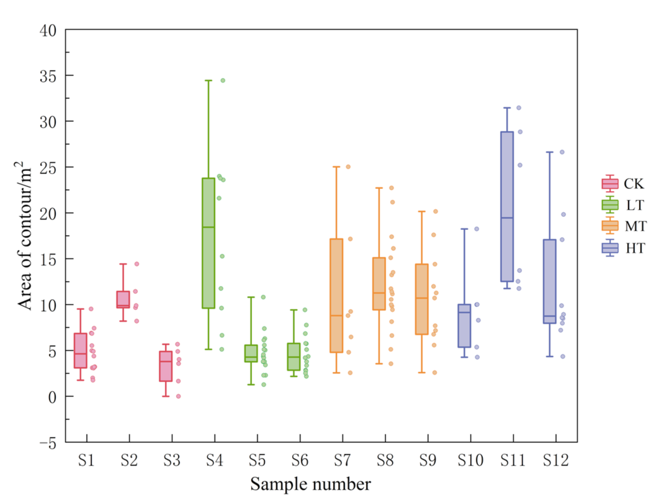
3.2.1. Effects of Thinning on Crown Area

For the crown area, the S11 plot had the highest mean value of 16.00 m² under the HT treatment (Figure 3). This indicated that branches and leaves had sufficient space to grow. In contrast, under the LT treatment, the mean A value of the S6 plot was the smallest. The S6 plot had been well-renewed, indicating more young trees. The mean values found for the CK, LT, MT, and HT treatments were 12.22, 8.25, 11.16, and 12.76 m², respectively. It was greatest under the HT treatment, which was 4.23%, 35.34% and 12.54% higher than the CK, LT and MT treatments, respectively. This indicates that the HT treatment is most conducive to canopy growth.

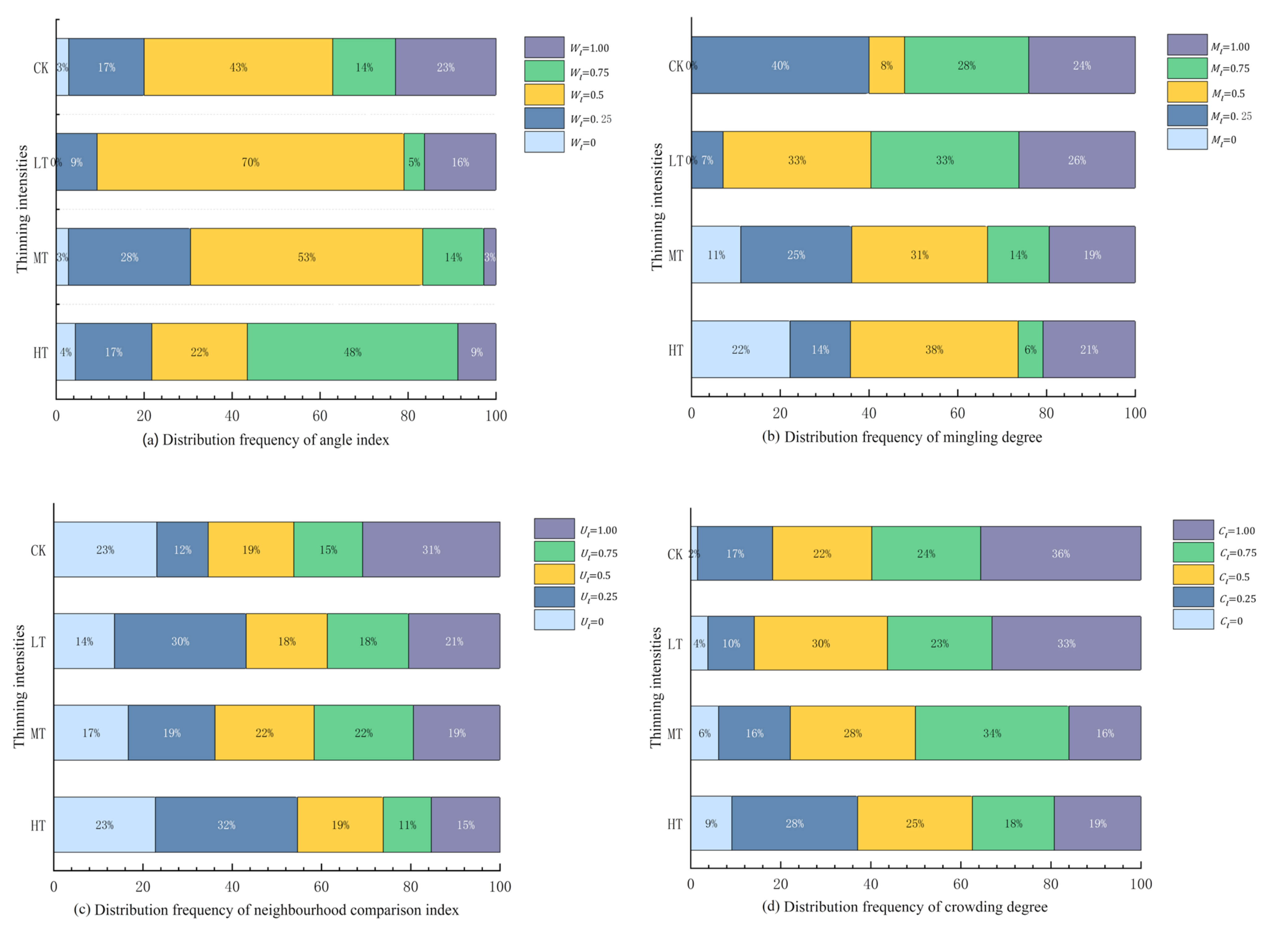
3.2.2. Effects of Thinning on Spatial Structure Index

Under the four treatments, the W value distributions differed with regard to their means (Figure 4a). The mean W values were 0.593, 0.570, 0.463, and 0.598 under the CK, LT, MT and HT treatments, respectively. We found that the mean W value increased and then decreased with increasing thinning intensity. The CK, LT and HT spatial distributions may be characterized as random. The MT spatial distribution was the closest to a uniform distribution. For the frequency distribution of five values, the proportion of the absolutely uniform (W = 0) and clumped distribution (W = 1) were small. The largest proportion of the CK, LT, MT treatments were distributed at random (W = 0.5). At the HT treatment, the trees were more unevenly distributed. Therefore, thinning needs to be appropriately adjusted.

The mean M values of the CK, LT, MT and HT treatments were 0.590, 0.696, 0.514, and 0.597, respectively (Figure 4b). The MT treatment was registered a moderate degree. The CK and HT treatments registered between a moderate and strong degree. In contrast, the spatial structure of the LT treatment tended to be strongly mixed. The frequency distribution reached a maximum when M = 0.25 under the CK treatment. This indicates that the same tree species are concentrated. As the thinning intensity increases, the frequency of M = 0 was gradually increased (CK: 0%, LT: 0%, MT: 11%, HT: 22%). The magnitude of species isolation is affected by thinning, and tree species are gradually monolithic. In order to increase species diversity, we need to develop reasonable plants and transformations.

In this experiment, the degree of mingling under each treatment was found to be moderate, with values ranging from 0.470 to 0.548. According to Figure 4c, the CK treatment had a larger proportion of advantaged trees (U = 0) and the largest proportion of absolutely disadvantaged (U = 1) trees. The distribution of trees shows that many reference trees are dominant in their immediate vicinity, whereas more trees are surrounded by four bigger neighbours. Under the MT treatment, there were many subadvantaged trees,; therefore, the maximum U value of the frequency distribution occurred at U = 0.25. However, under the MT treatment, the value was average at the five values. Under the CK, LT, and MT treatments, the mean U values all between 0.5 and 0.75. All species occurred as moderate or disadvantage trees in the three treatments. However, under the HT treatment, the mean U value was smaller compared to the other treatments, and the trees were not significantly differentiated. Finally, the growth status of the trees was in a moderate position.

The density of the trees could be efficiently changed by thinning. The C value contains certain competition information and visually expresses whether the canopy covers the ground continuously [30]. Thus, the smaller the values of the C-index are, the lower the competitive pressure is. The mean C values, which were 0.376, 0.343, 0.336 and 0.305, respectively (Figure 4d), decreased sequentially with an increase in thinning intensity. Under the CK, LT, and MT treatments, the cumulative frequency of C = 0.75 and C = 1 was more than 50%, indicating that the canopies are dense. Therefore, they have more overlapping parts. We need to adjust the forest density to increase the proportion of sparse and sparse trees.

3.3. Relationship between Spatial Structure Parameters and Carbon Stock under Different Treatments

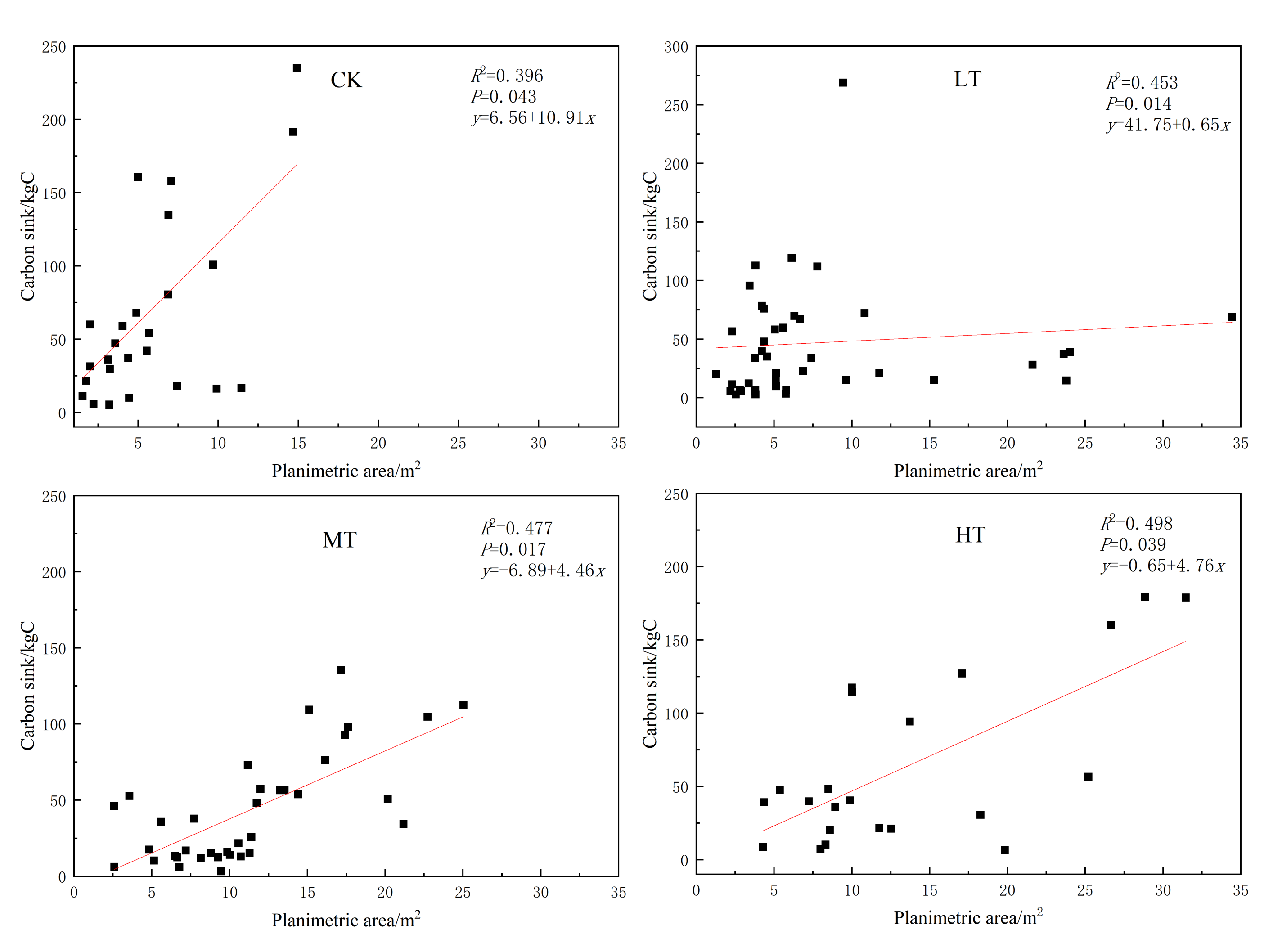
3.3.1. Relationship between Crown Area and Carbon Stock

Differences in crown area drive variation in individual tree carbon stock under all treatments (Figure 5). All the A values showed significant linearly positive correlations with the carbon stocks (p < 0.05). The slope of the fitted curve was maximum under the CK treatment. This indicates that carbon stock increases rapidly as crown area increases. The sequence of fitting was therefore as follows: HT (R² = 0.498), MT (R² = 0.477), LT (R² = 0.453) and CK (R² = 0.396). It appears that the canopy is most closely related to carbon stock at the heavily thinned intensity, but least closely at the control intensity.

3.3.2. Relationship between Spatial Structure Index and Carbon Stock

We correlated stand structure with carbon stock and drew some conclusions (

Table 3. The correlation analysis of spatial structure index and carbon stock.

Spatial Structure Index	Thinning Treatment	Number	Result
			r Value	p Value
W-index	CK	37	0.073	0.251
	LT	52	0.180	0.364
	MT	46	0.441	0.000
	HT	32	0.367	0.006
M-index	CK	37	0.096	0.268
	LT	52	0.379	0.000
	MT	46	0.167	0.002
	HT	32	0.198	0.006
U-index	CK	37	−0.160	0.027
	LT	52	−0.273	0.000
	MT	46	−0.194	0.002
	HT	32	−0.072	0.000
C-index	CK	37	−0.190	0.001
	LT	52	−0.056	0.000
	MT	46	−0.244	0.000
	HT	32	0.272	0.006

Note: The larger the value of |r|, the better the correlation. A positive number means positive correlation, whereas a negative number means negative correlation. The p-value is used to determine whether the correlation coefficient, r, is statistically significant or not, and the determination standard is generally 0.05.

). First, a detailed analysis between the uniform angle index and carbon stock indicated that they had a significant correlation (p < 0.01) under the MT and HT treatments. In contrast, they did not show significant correlation (p > 0.05) under the CK and LT treatments. Second, it was found that the correlation coefficient of the M value and carbon stock was, from large to small: LT (r = 0.379), HT (r = 0.198), MT (r = 0.167). Tree carbon stocks were found to be statistically significant except for under the CK treatment (p > 0.05). Thirdly, the U-index graded the carbon stocks of individual trees under different treatments. It was discovered that the carbon stocks decreased gradually when the U value increased (Figure 6a). All U values showed a significant or highly significant relationship with carbon stocks (CK treatment: p < 0.05; LT, MT and HT treatments: p < 0.01).Lastly, a detailed analysis between C-index and carbon stock indicated that they had a highly significant correlation (p < 0.01) under all treatments.

We graded the carbon stock of individual trees according to the value of W. Meanwhile, cumulative carbon stocks at different W values were calculated as a percentage of the total (Figure 6a). Under all treatments, the cumulative carbon stocks showed a trend of increasing and then decreasing with an increase in W value. Under the CK, LT and MT treatments, the proportion of cumulative carbon stocks all reached a peak in random distribution (W = 0.5), and then decreased. However, the proportions increased slightly in clumped distribution (W = 1) under the CK and LT treatments. The cumulative carbon stocks under the HT treatment peaked in nonuniform distribution (W = 0.75). Although the proportion of cumulative carbon stocks increased and then decreased under both MT and HT treatments, the correlation coefficient was greater under the MT treatment (r = 0.441), indicating that the W-index of this stand has a more significant effect on carbon stocks.

As shown in Figure 6b, there was no zero degree under the CK and LT treatments. Under the CK treatment, the carbon stock of individual trees was mostly concentrated at $M$ = 0.25. However, the cumulative carbon stocks did not change regularly as the value of $M$ increased. Under the LT treatment, the cumulative carbon stocks gradually increased with an increase in M value, and the largest proportion of cumulative carbon stocks was 39.11% to an extremely strong degree (M = 1). Under the MT and HT treatments, the cumulative carbon stocks increased with an increase in M value, and peaked to a moderate degree (M = 0.5), then steadily declined. A detailed analysis of cumulative carbon stocks indicated that more spatial resources are available for individual trees when in a low forest density. When the four nearest neighbor trees cannot form a good mixed state with the reference tree, the carbon tends to be stored in individuals who in a moderate degree state.

Under each treatment, carbon stocks of individual trees all reached peak when they were in advantaged positions (Figure 6c). We found that Abies fabri occupied absolute spatial and resource advantages. Hence, carbon tended to accumulate in the individuals in advantaged positions. Under the LT and MT treatments, the cumulative carbon stock was reduced as the U value increased. Under the CK and HT treatments, more carbon was accumulated in moderate individuals compared to subadvantage and disadvantage ones. Under the thinned treatments, the lowest cumulative carbon stocks were found at U = 1. This indicates that carbon hardly accumulates when an individual tree is at an absolute disadvantage.

Under the CK, LT and MT treatments, carbon tended to accumulate in the sparse areas (Figure 6d), because the sparse areas had sufficient light and rich abundant spatial resources. However, the cumulative carbon stocks of extremely sparse states were 14.3%, 8.1% and 21.0% less than those of sparse states. Under the HT treatment, the forest density was least. Therefore, the stand had weak competition, and carbon tended to accumulate in sparse (C = 0.25) and moderately dense (C = 0.5) areas. We found that the smallest proportion of cumulative carbon stocks was only 8.6%, 10.1%, 3.4% and 11.0% at C = 1 under all treatments.

4. Discussion

Forest structure has a significant impact on the functions of forests. A good forest structure is central in the sustainable operation of forests. The carbon sink function represents a major component of forest functions. Due to the lack of a relationship between forest structure and carbon sequestration function, it is difficult to accurately predict the tendency of carbon accumulation. Therefore, it is necessary to investigate the forest structure and carbon stocks under different thinning treatments. In this paper, we investigated a current and interesting topic: thinning effects on stand structure and carbon content of secondary forests. These are two important issues that not everyone tackles in connection with one another, but often individually. In this paper, we investigated the effects of four treatments on the stand structure (including: DBH structure, as well as A-, W-, M-, U- and C-indices) of a mixed conifer and broadleaf natural secondary forest. The results are extremely important for researchers to understand the effects of thinning on stand structure and carbon stock.

The Weibull distribution function was used to fit the DBH distribution, followed by statistical analysis and verification the results. Our study revealed that the Weibull function accurately simulated the DBH distribution under all treatments. The universality of the Weibull distribution application has been proved in a number of studies [33,34,35], and it was well demonstrated in this paper. The A-, W-, M-, U- and C-indices were analysed under four different treatments. Under the LT treatment, the lack of space resources in the upper space is not conducive to canopy growth. The HT treatment provided a large upper space for standers. The extension of branches and leaves was promoted, so resource utilization was increased. This result is consistent with the findings of P. Comeau et al. [36]. The crown area first increased and then decreased as the thinning intensities increased. If the W values fall in the interval of 0.475–0.517, it implies a random distribution pattern. Otherwise, the distribution pattern can be regular ($W$ < 0.475) or clumped ($W$ > 0.517) [37]. The MT treatment formed a stable structure and a regular distribution of trees. However, under the CK, LT and HT treatments, the trees need to be properly adjusted in order to achieve the best spatial distribution. This result contradicts the findings of several researchers [38,39], because it is related to a variety of factors, such as forest type, thinning intensity and tree species; The LT and HT treatments both enhanced the degree of spatial isolation of tree species, which was conducive to the increase in species [40]. This result is consistent with the study of Zhang, T et al. [38]. In addition, the mean U and C values decreased gradually as thinning intensities increase. This indicates that thinning reduces the size difference among trees and eliminates the absolute competitive advantage of large DBH trees. We can infer that forest competition pressure is gradually released as the thinning intensities increase. This is inconsistent with the research of Ye et al. [39], because the results were influenced by additional nutrition, forest type, time after thinning, and intensity of thinning.

The results paint a nuanced picture of variation between stand structure and carbon stock. Stand structure impacts forest carbon sinks by influencing precipitation, soil nutrients and understory light [41,42]. Under the CK, LT and MT treatments, the cumulative carbon stocks reached a peak when the trees were randomly distributed. In contrast, the cumulative carbon storage of trees peaked at a nonuniform distribution under the HT treatment. The renewed species were mostly concentrated around the remaining trees after heavily thinnin;, in this case, the stand shows a crumb carbon distribution structure. In general, carbon tends to accumulate in individuals with greater dominance. However, under the CK and HT treatments, the cumulative carbon stocks of moderate individuals were greater than those of subadvantageous individuals. Under the HT treatment, human disturbance factors were stronger than the factors, although the differentiation of the stand was not obvious. In this stand, more subadvantaged trees were removed by thinning, which reduced the cumulative carbon stock. In addition, each tree species has different maturity years and carbon sequestration abilities. We found that carbon tended to accumulate in sparse areas rather than extremely sparse areas under the CK, LT and MT treatments. Several reasons have been summarized by Martin et al. [43]. First, and perhaps most important, is a reduction in biodiversity and the destruction of microhabitat in overly sparse areas. Second, the extremely sparse state had too few trees around it to create a woodland microclimate, which is detrimental to its growth. Third, independent trees increase the probability of windfall. However, the HT treatment changed the tendency of carbon accumulation. This stand with low density has weak competition, and carbon tended to accumulate in sparse and moderately dense areas.

Our first hypothesis appears to be perfectly supported by the results. Thinning intensity affects stand structure of the mixed conifer and broadleaf natural secondary forest. In this paper, thinning concentrated the DBH distribution of trees. There are various indicators of spatial structure, including the A-, W-, M-, U- and C-indices. The values of A first decreased and then increased as the thinning intensities increased; Under the MT treatment, the mean value of W was reduced, which enhanced the cluster distribution of trees. The mean M values might be improved by the LT and MT treatments. With an increase in thinning intensity, the mean U and C values tended to decrease gradually. As a result, the competitive pressure of the stand decreased. Our second hypothesis that the tendency of carbon accumulation varies under different thinning intensities was also perfectly supported by our results. Carbon tends to accumulate in individual with a random distribution, a sparse space, strong mingling index and large competitive advantages; this was the same as Cui’s conclusion [44]. However, the tendency of carbon accumulation varied under different treatments. In this study, the tendency of carbon accumulation under the CK treatment was different from that under other treatments, and the most carbon accumulated in the weak degree state. In general, carbon tends to accumulate in advantage individuals, but it tended to accumulate in a nonuniform distribution, subadvantaged position and moderately dense individuals under the HT treatment.

The stand structure characteristics of natural secondary forests are very complex. The stands set up in the Small Khingan Mountains can only represent the growth regularities in this range. Thus, the results have some limitations. In the future, we should add other representative areas to make the research data more comprehensive. Additionally, stand structure is a dynamic process of long-term change. We will extend the restoration years for longer-term observation and analysis. We can also add some research on shrubs and herbs to form different hierarchical relationships and network structures. Making carbon sink in long-lasting reforestation is a widely embraced carbon sequestration technique [45]. If possible, we will carry out replanting of tree species.

5. Conclusions

The thinning treatments had clear effects on the stand structure accounting for the A-, W-, M-, U- and C-indices. We also explored the relationship between stand structure indicators and carbon stock. The results showed that the trees under the CK treatment were dense and in a clustered distribution. There were more advantage individuals and the most absolutly disadvantage ones. Meanwhile, DBH differentiation was obvious in this stand. Under the LT treatment, the canopy did not have sufficient growing space, so the crown area was minimized. In this stand, tree species isolation was strongest, which was conducive to the increase in species diversity. Under the MT treatment, the trees were evenly distributed, and the structure was more stable. However, the MT stand was weakly mixed. Manual intervention is needed to plant other associated tree species to improve biodiversity; The canopy growth space was sufficient under the HT treatment. In this stand, the mingling degree was between moderate and strong. Many advantage and subadvantage trees grew sturdily. However, some trees were unevenly distributed. We need to appropriately regulate the stand so that the distribution is random.

Under all treatments, there was a significant positive correlation between the carbon stock of an individual tree and its crown area. Carbon tends to accumulate in individuals with in random distribution, sparse space, strong mingling index and large competitive advantages. However, the tendency of carbon accumulation varied under different treatments. Individuals in a better position have access to more resources and ecological niches, so they accumulate carbon easily. From the vertical space perspective, we can increase the utilization efficiency of the resources by increasing the staggered space of the stand. Reasonably increasing or decreasing the mingling ratio of non-top communities is beneficial to accumulate carbon.

References

1. Pastorella, F.; Paletto, A. Stand structure indices as tools to support forest management: An application in Trentino forests (Italy). J. For. Sci. 2013, 59, 159–168. [Google Scholar] [CrossRef] [Green Version]
2. McElhinny, C.; Gibbons, P.; Brack, C.; Bauhus, J. Forest and woodland stand structural complexity: Its definition and measurement. For. Ecol. Manag. 2005, 218, 1–24. [Google Scholar] [CrossRef]
3. Brassard, B.W.; Chen, H.Y.H. Stand Structural Dynamics of North American Boreal Forests. Crit. Rev. Plant Sci. 2006, 25, 115–137. [Google Scholar] [CrossRef]
4. DeWalt, S.J.; Maliakal, S.K.; Denslow, J.S. Changes in vegetation structure and composition along a tropical forest chronosequence: Implications for wildlife. For. Ecol. Manag. 2003, 182, 139–151. [Google Scholar] [CrossRef]
5. Rahman, M.M.; Nishat, A.; Rahman, G.M.M.; Ruprecht, H.; Vacik, H. Analysis of spatial diversity of sal (Shorea robusta Gaertn.f) forests using neighbourhood-based measures. Community Ecol. 2008, 9, 193–199. [Google Scholar] [CrossRef]
6. Zhang, M.M.; Fan, S.H.; Yan, X.R.; Zhou, Y.Q.; Guan, F.Y. Relationships between stand spatial structure characteristics and influencing factors of bamboo and broad-leaved mixed forest. J. For. Res. 2020, 25, 83–91. [Google Scholar] [CrossRef]
7. Kohyama, T.; Aiba, S. Dynamics of primary and secondary warm-temperate rain forests in Yakushima Island. Tropics 1997, 6, 383–392. [Google Scholar] [CrossRef] [Green Version]
8. Liu, L.; Zeng, F.P.; Song, T.Q.; Wang, K.L.; Du, H. Stand Structure and Abiotic Factors Modulate Karst Forest Biomass in Southwest China. Forests 2020, 11, 443. [Google Scholar] [CrossRef] [Green Version]
9. Neil, G.; Williams, M.D.P. Carbon storage implications of active management in mature Pseudotsuga menziesii forests of western Oregon. For. Ecol. Manag. 2019, 432, 761–775. [Google Scholar] [CrossRef]
10. Huang, X.M.; Liu, S.R.; Wang, H.; Hu, Z.D.; Li, Z.G.; You, Y.M. Changes of soil microbial biomass carbon and community composition through mixing nitrogen-fixing species with Eucalyptus urophylla in subtropical China. Soil Biol. Biochem. 2014, 73, 42–48. [Google Scholar] [CrossRef]
11. Ali, A.; Lin, S.L.; He, J.K.; Kong, F.M.; Yu, J.H.; Jiang, H.S. Climate and soils determine aboveground biomass indirectly via species diversity and stand structural complexity in tropical forests. For. Ecol. Manag. 2019, 432, 823–831. [Google Scholar] [CrossRef]
12. Forrester, D.I.; Bauhus, J. A Review of Processes Behind Diversity—Productivity Relationships in Forests. Curr. For. Rep. 2016, 2, 45–61. [Google Scholar] [CrossRef] [Green Version]
13. Montoro, G.M.; Morin, H.; Lussier, J.M.; Walsh, D. Radial growth response of black spruce stands ten years after experimental shelterwoods and seed-tree cuttings in boreal forest. Forests 2016, 7, 240. [Google Scholar] [CrossRef] [Green Version]
14. Moussaoui, L.; Leduc, A.; Girona, M.M.; Bélisle, A.C.; Lafleur, B.; Fenton, N.J.; Bergeron, Y. Success factors for experimental partial harvesting in unmanaged boreal forest: 10-year stand yield results. Forests 2020, 11, 1199. [Google Scholar] [CrossRef]
15. Montoro, G.M.; Lussier, J.M.; Morin, H.; Thiffault, N. Conifer regeneration after experimental shelterwood and seed-tree treatments in boreal forests: Finding silvicultural alternatives. Front. Plant Sci. 2018, 9, 1145. [Google Scholar] [CrossRef]
16. Montoro, G.M.; Morin, H.; Lussier, J.M.; Ruel, J.C. Post-cutting mortality following experimental silvicultural treatments in unmanaged boreal forest stands. Front. For. Glob. Change 2018, 9, 1145. [Google Scholar] [CrossRef] [Green Version]
17. Bose, A.K.; Weiskittel, A.; Kuehne, C.; Wagner, R.G.; Turnblom, E.; Burkhart, H.E. Tree-level growth and survival following commercial thinning of four major softwood species in North America. For. Ecol. Manag. 2018, 427, 355–364. [Google Scholar] [CrossRef]
18. Kim, S.; Axelsson, E.P.; Girona, M.M.; Senior, J.K. Continuous-cover forestry maintains soil fungal communities in Norway spruce dominated boreal forests. For. Ecol. Manag. 2021, 480, 118659. [Google Scholar] [CrossRef]
19. Liu, C.X.; Wang, Y.J.; Ma, C.; Wang, Y.Q.; Zhang, H.L.; Hu, B. Quantifying the effect of non-spatial and spatial forest stand structure on rainfall partitioning in mountain forests, Southern China. For. Chron. 2018, 94, 162–172. [Google Scholar] [CrossRef]
20. Zhao, Q.Y.; Yu, K.Y.; Xiang, J.; Lin, L.L.; Huang, H.; Xie, Q.Y.; Liu, J. Influence of forest park stand structure characteristics on spatial thermal environment. J. Fujian Agric. For. Univ. (Nat. Sci. Ed.) 2019, 48, 48–54. (In Chinese) [Google Scholar]
21. Wang, Z.C.; Li, Y.X.; Meng, Y.B.; Wang, C. Effect of tending and thinning on spatial and carbon distribution patterns of natural mixed broadlesf-conifer secondary forest in Xiaoxing’an Mountains, PR China. Appl. Ecol. Environ. Res. 2021, 19, 4751–4764. [Google Scholar] [CrossRef]
22. Wang, Z.C.; Li, Y.X.; Meng, Y.B.; Wang, C. Responses of spatial distribution patterns and associations of Larix gmelinii and Populus davidiana mixed forests in Daxing’an Mountains to different tending thinning intensities. J. Cent. South Univ. For. Technol. 2022, 42, 75–83. (In Chinese) [Google Scholar]
23. Zhang, T.; Zhu, Y.J.; Dong, X.B. Effects of thinning on the habitat of natural mixed broadleaf-conifer secondary forest in Xiaoxing’an Mountains of northeastern China. J. Beijing For. Univ. 2017, 39, 1–12. (In Chinese) [Google Scholar]
24. Saka, M.G. Characterization of diameter distribution and prediction of Weibull parameters equation for plantation-grown Eucalyptus species. Asian J. Res. Agric. For. 2021, 7, 1–13. [Google Scholar] [CrossRef]
25. Ganbaatar, B.; Jamsran, T.; Gradel, A.; Sukhbaatar, G. Assessment of the effects of thinnings in scots pine plantations in Mongolia: A comparative analysis of tree growth and crown development based on dominant trees. For. Sci. Technol. 2021, 17, 135–143. [Google Scholar] [CrossRef]
26. Hui, G.Y. The neighbourhood pattern—A new structure parameter describing distribution of forest tree position. Sci. Silvae Sin. 1999, 35, 37–42. (In Chinese) [Google Scholar]
27. Hui, G.Y.; Hu, Y.B. Measuring species spatial isolation in mixed forests. For. Res. 2001, 14, 23–27. (In Chinese) [Google Scholar]
28. Hui, G.Y.; Hu, Y.B.; Zhao, Z.H. Evaluating tree species segregation based on neighborhood spatial relationships. J. Beijing For. Univ. 2008, 30, 131–134. (In Chinese) [Google Scholar]
29. Hui, G.Y.; von Gadow, K.; Albert, M. A new parameter for stand spatial structure neighbourhood comparison. For. Res. 1999, 12, 1–6. (In Chinese) [Google Scholar]
30. Hu, Y.B.; Hui, G.Y. How to describe the crowding degree of trees based on the relationship of neighboring trees. J. Beijing For. Univ. 2015, 37, 1–8. (In Chinese) [Google Scholar]
31. Hu, H.Q.; Luo, B.Z.; Wei, S.J.; Wei, S.W.; Sun, L.; Luo, S.S.; Ma, H.B. Biomass carbon density and carbon sequestration capacity in seven typical forest types of the Xiaoxing’an Mountains, China. Chin. J. Plant Ecol. 2015, 39, 140–158. (In Chinese) [Google Scholar]
32. Wang, C.K. Biomass allometric equations for 10 co-occurring tree species in Chinese temperate forests. For. Ecol. Manag. 2006, 222, 9–16. [Google Scholar] [CrossRef]
33. Zhang, L.J.; Liu, C.M. Fitting irregular diameter distributions of forest stands by Weibull, modified Weibull, and mixture Weibull models. J. For. Res. 2006, 11, 369–372. [Google Scholar] [CrossRef]
34. Zhang, M.T.; Kang, X.G.; Guo, W.W.; Meng, J.H.; Yang, Y.J. Diameter structural distribution of spruce-fir mixed forest in Changbai Mountain. J. Northwest A F Univ. Nat. Sci. Ed. 2015, 43, 65–72. (In Chinese) [Google Scholar]
35. Poudel, K.P.; Cao, Q.V. Evaluation of Methods to Predict Weibull Parameters for Characterizing Diameter Distributions. For. Sci. 2013, 59, 243–252. [Google Scholar] [CrossRef]
36. Philip, G.C. Effects of Aspen and spruce density on size and number of lower branches 20 years after thinning of two boreal mixedwood stands. Forests 2021, 12, 211. [Google Scholar] [CrossRef]
37. Zhang, G.Q.; Hui, G.Y.; Zhao, Z.H.; Hu, Y.B.; Wang, H.X.; Liu, W.Z.; Zang, R.G. Composition of basal area in natural forests based on the uniform angle index. Ecol. Inform. 2018, 45, 1–8. [Google Scholar] [CrossRef]
38. Zhang, T.; Dong, X.B.; Guan, H.W.; Meng, Y.; Ruan, J.F.; Wang, Z.Y. Effect of Thinning on the Spatial Structure of a Larix gmelinii Rupr. Secondary Forest in the Greater Khingan Mountains . Forests 2018, 9, 720. [Google Scholar] [CrossRef] [Green Version]
39. Ye, S.X.; Zheng, Z.R.; Diao, Z.Y.; Ding, G.D.; Bao, Y.F.; Liu, Y.D.; Gao, G.L. Effects of thinning on the spatial structure of Larixprincipis-rupprechtii plantation. Sustainability 2018, 10, 1250. [Google Scholar] [CrossRef] [Green Version]
40. Pretzsch, H. Mixing degree, stand density, and water supply can increase the overyielding of mixed versus mono specific stands in Central Europe. For. Ecol. Manag. 2021, 503, 119741. [Google Scholar] [CrossRef]
41. Fotis, A.T.; Murphy, S.J.; Ricart, R.D.; Krishnadas, M.; Whitacre, J.; Wenzel, J.W.; Queenborough, S.A.; Comita, L.S. Above-ground biomass is driven by mass-ratio effects and stand structural attributes in a temperate deciduous forest. J. Ecol. 2018, 106, 561–570. [Google Scholar] [CrossRef]
42. Capellesso, E.S.; Scrovonski, K.L.; Zanin, E.M.; Hepp, L.U.; Bayer, C.; Sausen, T.L. Effects of forest structure on litter production, soil chemical composition and litter-soil interactions. Acta Bot. Bras. 2016, 30, 329–335. [Google Scholar] [CrossRef]
43. Martin, M.; Raymond, P. Assessing tree-related microhabitat retention according to a harvest gradient using tree-defect surveys as proxies in Eastern Canadian mixedwood forests. For. Chron. 2019, 95, 157–170. [Google Scholar] [CrossRef] [Green Version]
44. Cui, S.; Xiao, R.; Wang, W.F.; Liu, B.F. The study on the structural characteristics of the mixed-wood carbon sink in Xiaoxinganling Area. For. Eng. 2020, 36, 30–35. (In Chinese) [Google Scholar]
45. Ameray, A.; Bergeron, Y.; Valeria, O.; Montoro, G.M.; Cavard, X. Forest Carbon Management: A Review of Silvicultural Practices and Management Strategies Across Boreal, Temperate and Tropical Forests. Curr. For. Rep. 2021, 7, 245–266. [Google Scholar] [CrossRef]
Figure 1. (a) The locations of the studied forest stands in the Small Khingan Mountains in China, (b) in which 4 stands represent.different thinning treatments, (c) contains characteristics of the stands.
Forests 13 00512 g001
Figure 2. DBH frequency of Weibull distribution under different treatments. The results were subjected to χ2 test, and then the fitting results were analysed.
Forests 13 00512 g002
Figure 3. The effect of thinning on A-index under different treatments. The CK treatment included plots S1~S3, the LT treatment included plots S4~S6, the MT treatment included plots S7~S9, and the HT treatment included plots S10~S12.
Forests 13 00512 g003
Figure 4. Distribution frequency of spatial structure index under different treatments. Pictures (ad) represent angel index, mingling degree, neighbourhood comparison index and crowing degree, respectively.
Forests 13 00512 g004
Figure 5. Relationship between crown area and carbon stock under different treatments.
Forests 13 00512 g005
Figure 6. The carbon proportion of spatial structure index under different treatments. Pictures (ad) represent uniform angel index, mingling degree, neighbourhood comparison and crowing degree, respectively.
Forests 13 00512 g006