Article

Forest Damage by Extra-Tropical Cyclone Klaus-Modeling and Prediction

1
Institute of Earth Sciences, Faculty of Natural Sciences, University of Silesia in Katowice, ul. Będzińska 60, 41-200 Sosnowiec, Poland
2
International Environmental Doctoral School, University of Silesia, ul. Będzińska 60, 41-200 Sosnowiec, Poland
*
Author to whom correspondence should be addressed.
Forests 2022, 13(12), 1991; https://doi.org/10.3390/f13121991
Submission received: 10 October 2022 / Revised: 17 November 2022 / Accepted: 23 November 2022 / Published: 25 November 2022
(This article belongs to the Special Issue Impact of Climate Warming and Disturbances on Forest Ecosystems)

Abstract

:
Windstorms may have negative consequences on forest ecosystems, industries, and societies. Extreme events related to extra-tropical cyclonic systems remind us that better recognition and understanding of the factors driving forest damage are needed for more efficient risk management and planning. In the present study, we statistically modelled forest damage caused by the windstorm Klaus in south-west France. This event occurred on 24 January 2009 and caused severe damage to maritime pine (Pinus pinaster) forest stands. We aimed at isolating the best potential predictors that can help to build better predictive models of forest damage. We applied the random forest (RF) technique to find the best classifiers of the forest damage binary response variable. Five-fold spatial block cross-validation, repeated five times, and forward feature selection (FFS) were applied to the control for model over-fitting. In addition, variable importance (VI) and accumulated local effect (ALE) plots were used as model performance metrics. The best RF model was used for spatial prediction and forest damage probability mapping. The ROC AUC of the best RF model was 0.895 and 0.899 for the training and test set, respectively, while the accuracy of the RF model was 0.820 for the training and 0.837 for the test set. The FFS allowed us to isolate the most important predictors, which were the distance from the windstorm trajectory, soil sand fraction content, the MODIS normalized difference vegetation index (NDVI), and the wind exposure index (WEI). In general, their influence on the forest damage probability was positive for a wide range of the observed values. The area of applicability (AOA) confirmed that the RF model can be used to construct a probability map for almost the entire study area.

1. Introduction

Windstorms can bring devastating energy over Europe and a number of negative consequences to terrestrial ecosystems, soil cover, industry, and society [1,2]. It is estimated that annual losses to the EU and the UK are as high as 5 billion EUR, or approximately 0.04% of the total GDP [3]. Due to such a high level of losses, the problem of windstorm-related geohazards and disturbances requires serious consideration and new tools and methods, particularly in the context of the potential effects of climate change [4,5,6]. Extra-tropical windstorms have been studied for decades, and their impact on forests can be modelled and predicted to some extent [7,8,9]. To date, two types of models have been proposed: (1) hybrid-mechanistic and (2) statistical/machine learning models [10,11,12]. Hybrid-mechanistic models are based on information regarding the biomechanical behavior of trees under the forces generated by wind currents and information related to local and regional wind regimes [10,13]. Wind-related data can be obtained from models approximating the airflow over complex terrain, such as WindStation [14]. One example is the ForestGALES model, which is based on critical wind speed data and a windiness scoring system that allows the prediction of the probability of forest damage [13,15]. The best mechanistic models, such as ForestGALES or HWIND, are able to make predictions at a high level of accuracy if they have been parameterized for specific tree species [16,17]. Statistical/machine learning methods allow a certain degree of generalization based on large datasets and repeated evaluation of model training results, (e.g., in the case of k-fold cross-validation). Both approaches offer some advantages, but they also have limitations. Hybrid-mechanistic models can be sensitive to input data (such as expected wind speed or tree height), while statistical/machine learning models may be site-specific and sometimes do not work sufficiently well for new data [10].
Wind (speed, gustiness, direction) is the most difficult climate variable to model and predict due to its high dynamics (measured in seconds) and a wide range of factors influencing its properties. At the same time, wind is a key climatic agent affecting forest stand structures and dynamics, across the world, in both managed and old-growth forests. This has been reported in numerous scientific studies that have provided evidence of forest damage caused by strong winds [18,19,20,21,22].
It is commonly believed that the magnitude and frequency of catastrophic winter windstorms have recently increased, and this trend is predicted to continue, with a negative impact on forests [4,21,23,24]. However, there are contrasting opinions about the main drivers of the increase in storms and the scale of forest disturbance. For instance, Schelhaas et al. [23] concluded that the average volume of forest growing stock in Europe increased (along with forest area and stand age), thus increasing forest vulnerability to damage. This corresponds to the conclusions formulated by Seidl et al. [24], who also underlined the increasing standing timber volume that strongly influenced its susceptibility to disturbances. These findings agree with [9], who found that tree biomass was the most important predictor of forest damage in the Sudety Mountains in Poland [9]. However, other studies have reported increased storminess, which may have caused increased forest damage over the past decades [21]. This corresponds to the previous synthesis by Ranson et al. [4], who found, based on a literature review, that whilst the number of extra-tropical cyclones in the northern hemisphere may decrease, the number of extreme (very low pressure) winter cyclones may increase in certain regions. Nonetheless, Spinoni et al. [3] did not find any robust increasing trends in European windstorms. Assuming 3 °C warming (under RCP8.5; Representative Concentration Pathway), 16% of the land area in Europe may experience reduced maximum wind speeds. At the same time, the maximum wind speeds may increase in over 10% of Europe (including in the Alps), while remaining stable over the rest of the continent [3]. Under this climate scenario, wind losses may reach 4.6 billion EUR, annually. In the climate context, it seems the most dangerous are clusters of extreme events, which in terms of extra-tropical cyclones, mean several cyclones moving one after another in a short period of time [25].
Windstorm Klaus was a devastating event that caused severe damage to European forests, particularly in the Aquitaine region of France on 24 January 2009. It is estimated that it damaged 42 Mm3 of trees, mainly maritime pine (Pinus pinaster) [26]. The total financial loss for these stands was estimated at ca 1.5 billion EUR in France alone [26]. Liberato et al. [27], based on a report by Aon-Benfield [28], claimed that the windstorm was the costliest weather hazard event, globally, in 2009, causing damage in France, Spain, and Portugal that was estimated between 4.0 and 6.0 billion USD. The Extreme Wind Storms Catalogue (http://www.europeanwindstorms.org/, accessed on 1 October 2022) showed that windstorm Klaus was the sixth most damaging event between 1987 and 2013 in terms of insured loss (3.5 billion USD). This event also killed at least 26 people [28].
With the increasing uncertainty regarding the magnitude of changes in wind properties and storm occurrence, and their severity under different climate change scenarios, a better understanding of the vulnerability of forests is needed. From the viewpoint of forest management ecology, this is a key issue in many European countries. In the present study, we aimed to contribute to the understanding of the negative consequences of extra-tropical cyclones on forest ecosystems. To explain the spatial distribution of wind-related forest damage, we applied one of the most efficient machine learning techniques, the random forest (RF) method [9]. We used it for the first time to model forest damage caused by the windstorm Klaus in 2009 in southwest France. We selected windstorm Klaus due to the relatively large database, with detailed information on forest damage during the event that allowed us to construct more robust prediction models. We aimed to isolate and calculate the impact of the most important predictors to support the construction of wind damage probability maps.
We describe the study area (Section 2.1) and explain how we define the response variable (Section 2.3.1). The method of selection and preparation of the set of potential predictors is presented in Section 2.3.2 and Section 2.3.3. All steps of our modelling approach are elaborated in Section 2.4. The results are included in Section 3, and thoroughly discussed in Section 4, followed by our recommendations and conclusions in Section 5.

2. Materials and Methods

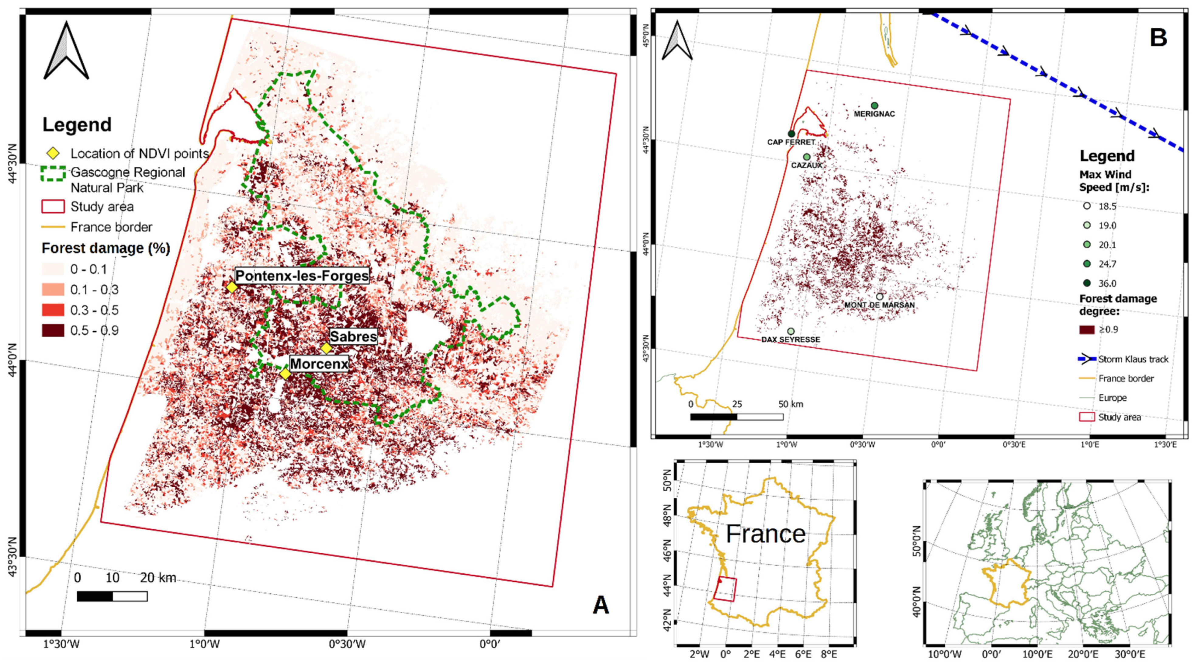
2.1. Study Area—Physical Settings and Climate

The study area is in southwest France, in the Nouvelle Aquitaine administrative region and the Gascony historical region. It is bordered, to the west, by the Bay of Biscay, which is part of the Atlantic Ocean (Figure 1). The relief has a lowland character, with small differences in the relative altitude (up to 250 m). Limestone and marl plateaus comprise the bedrock in the north, while sandstone and conglomerates form the so-called molasse in the south. A major part of the study area is dominated by podzols underlined by an impermeable layer of iron pan or bedrock [29].
According to the Koppen-Geier climate classification [31], the climate of the area under study is temperate and oceanic, with hot summers and no dry season (Cfb). The mean annual temperature in Cazaux is +13.4 °C (+6.6 °C in January, +20.6 °C in July), while in Mont de Marsan the mean annual temperature is +13.2 °C (+5.7 °C in January, +21.1 °C in July). The mean total annual precipitation is 862 mm and 844 mm in Cazaux and Mont de Marsan, respectively [32]. The mean annual wind speed in Cazaux is 3.2 m s−1 (3.2 m s−1 in January, 3.3 m s−1 in July); in Mont de Marsan the mean annual wind speed is 2.4 m s−1 (2.2 m s−1 in January, 2.5 m s−1 in July).
Windstorm Klaus developed from a small wave perturbation on 21 January and intensified on 23 January 2009, moving rapidly towards the Bay of Biscay [27]. The system underwent explosive development when crossing the polar jet at an unusually low latitude position [27]. According to the data provided by the NOAA (National Oceanic and Atmospheric Administration) [32], the maximum wind speed during windstorm Klaus reached 36 m s−1, on 24 January 2009. However, other sources reported that the wind speed was over 44 m s−1 [27].

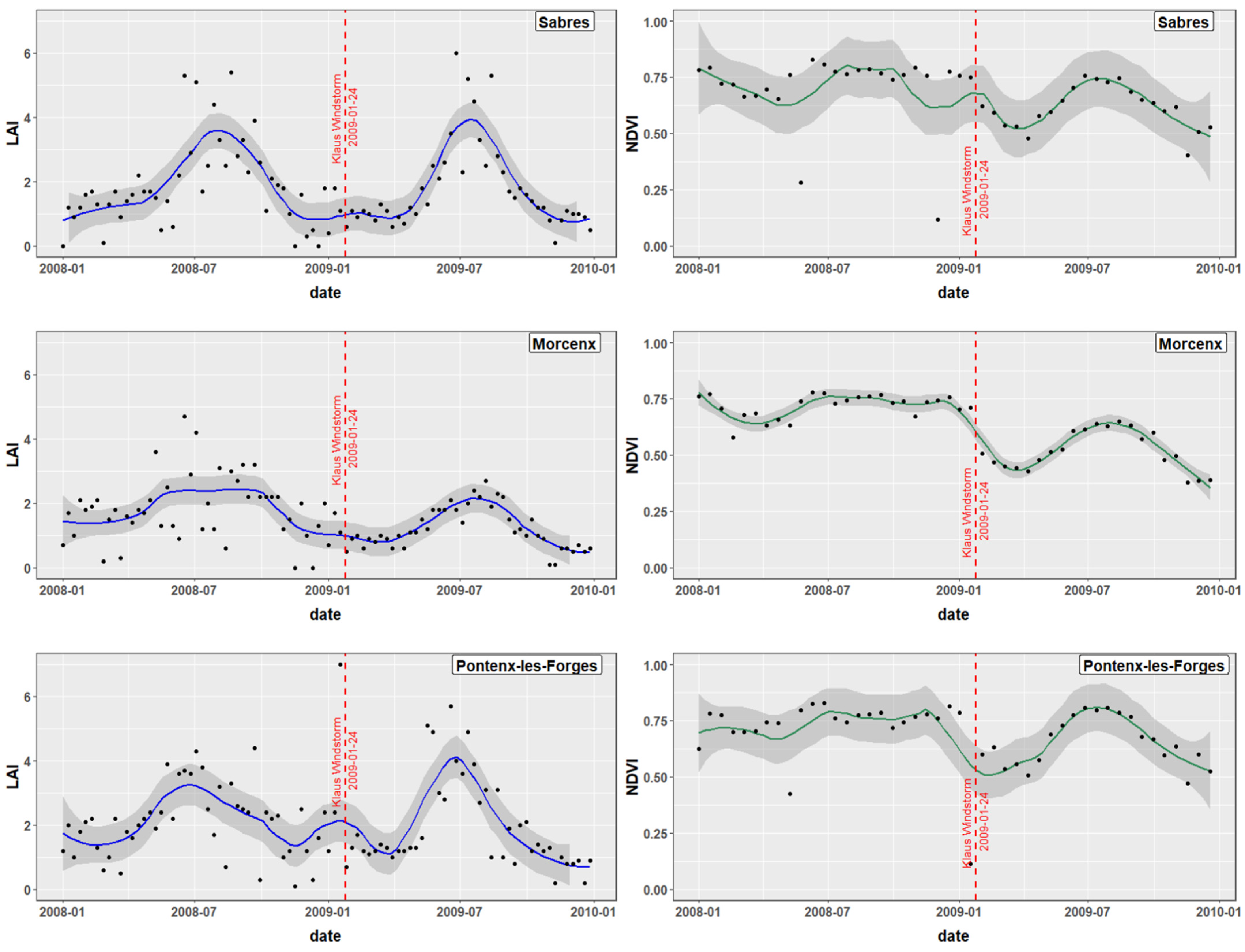
2.2. Forest Conditions before and after Windstorm Klaus

The area of interest (AOI) was originally occupied by heath and marshes. Currently, most of the area is made up by the Landes forest, which is considered to be one of the largest man-made woodlands in Western Europe. The forests were planted in the 18th and 19th centuries to combat erosion and rehabilitate landscapes, as well as to provide wood for industrial purposes. The dominant species was the maritime pine (Pinus pinaster). The central part of the Landes forest area is protected by the Landes de Gascogne Regional Natural Park, established in 1970. Part of the study area is also used for agriculture, mainly for grain farming [29,33]. The data in the Forest Global Change web service (https://glad.earthengine.app/view/global-forest-change#dl=1;old=off;bl=off;lon=20;lat=10;zoom=3; accessed on 1 October 2022) did not show any spectacular damage in that part of France between 2000 and 2008 [34]. However, other data sources indicate that forests in the area were damaged during a storm on 27 December 1999 [35]. The affected region was between Bordeaux and the Atlantic coastline, with a damage level exceeding 30% of the forest area in each forest inspectorate [35]. The event resulted in estimated losses of 26.0 Mm3 of wood [36]. It is likely that because of the 1999 event, damage caused by windstorm Klaus was much lower in that region than in the southern part of the AOI. The Leaf Area Index (LAI) and NDVI time series were inspected to obtain a better understanding of the forest stand conditions before and after windstorm Klaus (Figure 2). The NDVI decreased after the Klaus windstorm, and its values were lower than those in the same period during 2008. For the same points, the LAI showed only a sudden drop in the area close to Pontenx-les-Forges. Essentially, there are no clearly visible negative outcomes of the windstorm Klaus in the LAI graphs. Two plots (Sabres and Pontenx-les-Forges) showed even higher LAI values for July 2009 than a year before. Based on this exploratory analysis, it was decided that NDVI would likely be a better metric for exploring the impacts of windstorm Klaus on the region’s forests. This was tested in the training module of the present project.

2.3. Data Sources and Pre-Processing

2.3.1. Response Variable

Information concerning the forest damage caused by windstorm Klaus was obtained from the dataset compiled by Forzieri et al. [30]. The FORWIND dataset consists of information on wind disturbances in European forests from 2000 to 2018. It includes almost 90,000 records of areas disturbed by strong winds. The response variable was defined in the database as the degree of damage (D). The D has five classes and single values ascribed to those classes: 0.1 (D ≤ 20%), 0.3 (20% < D ≤ 40%), 0.5 (40% < D ≤ 60%), 0.7 (60% < D ≤ 80%), and 0.9 (80% < D ≤ 100%) (Table S1, Supplementary Materials). For data related to windstorm Klaus, this classification was based on the interpretation of aerial images obtained by the Institut National de information geographique et forestiere. In total, the FORWIND database consists of 21,691 records related to windstorm Klaus (polygons with determined degree of damage). Most of the damage was concentrated along the Atlantic Ocean coastline between Bordeaux, Mont de Marsan, and Dax. The damage area included the Landes de Gascogne Regional Natural Park (Figure 1).

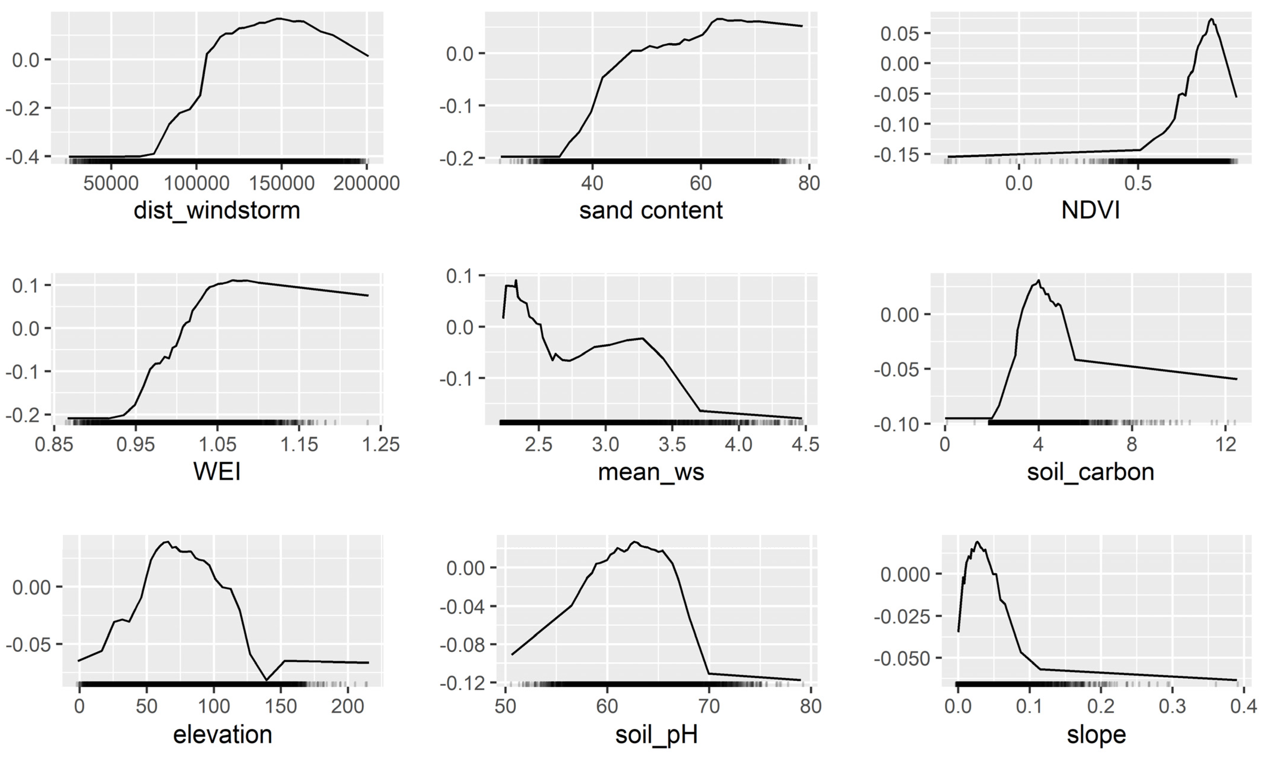
2.3.2. Potential Environmental Predictors

In this study, we used four types of potential predictors: (1) climate; (2) geomorphic; (3) soil properties; and (4) vegetation indices (Table 1).
The climate predictors included information on wind speed. The first wind speed layer used is a product offered by the Windstorm Information Service (WISC) that contains spatial data on the most significant European windstorms since 1940. In that service, storm tracks, footprints, summary data and loss estimates are based on the ERA5 (ECMWF Reanalysis 5th Generation, ECMWF stands for European Centre for Medium-Range Weather Forecasts) reanalysis data sets. The windstorm Klaus footprint was a gridded dataset showing a maximum three-second wind gust speed (in m s−1) at each grid point during the entire 72 h storm period. The wind speed layer used was available as a NC (NetCDF–Network Common Data Form) file.
The second wind-related predictor was the mean wind speed in January, calculated from gridded data for the based period 1999–2008, i.e., prior to windstorm Klaus in 2009. In addition, we used the January 2009 wind speed. The data were downloaded from the Climatology Lab web service (https://www.climatologylab.org/terraclimate.html, accessed on 1 October 2022).
In machine learning models, the most commonly used geomorphic variable is elevation, which is used for the calculation of other terrain properties, e.g., slope, terrain roughness, etc. We used the EU-DEM v1.1 elevation data, downloaded from the Copernicus web service (Table 1). The data can be downloaded in the 1000 × 1000 km tiles as zipped GeoTIFF files. The initial resolution was 25 m (vertical accuracy ± 7 m RMSE), and the layer is available in ETRS89-LAEA (European Terrestrial Reference System 1989—Lambert Azimuthal Equal-Area) projection (EPSG:3035). The digital elevation model was used to calculate the terrain roughness, profile and planform curvature, topographic wetness index (TWI), and wind exposure index (WEI). The terrain slope, roughness, profile, and planform curvature were calculated using the raster R package [38]. For the slope calculation, the package follows Horn’s [39] method. Terrain roughness is defined as the difference between the maximum and minimum cell values of a cell and the eight surrounding cells. The profile and planform curvatures were calculated using the spatialEco R package [40]. The planform and profile curvatures are the second derivatives of terrain elevation, or slope of the slope. The TWI and WEI were calculated using the SAGA GIS software 7.9.1 [41]. TWI is a dimensionless index that describes the potential surface water flow and accumulation [42]. The WEI provides information about terrain exposure to potential airflow where places with WEI < 1 are shadowed from the potential influence of airflow, and places with WEI > 1 are exposed to wind impact. The TWI and WEI were previously used in ecological and geomorphic modelling [9,43].
Soil properties are commonly considered an important type of information for environmental modelling, including the modelling of wind-related damage [12,20]. We used five types of soil feature data, measured at 10 cm depth: (1) sand; (2) clay fraction; (3) soil pH; (4) soil bulk density; and (5) soil organic carbon content. Raster layers containing information on soil properties were the result of ensemble machine learning modelling on a large set of reference points [44] and were made available as open-source data through the OpenLandMap web service (https://openlandmap.org/, accessed on 1 October 2022).
We applied two vegetation indices: the Leaf Area Index (LAI) [45] and the normalized difference vegetation index (NDVI), calculated from the Moderate Resolution Imaging Spectroradiometer (MODIS) satellite images. These two products were accessed using the MODISTools 1.1.2 R package [37]. The LAI is defined as the one-sided green leaf area (m2) per unit ground area (m2) in broadleaf canopies, and one-half of the total needle surface area per unit ground area in coniferous canopies (https://lpdaac.usgs.gov/products/mcd15a2hv006/, accessed on 1 October 2022). These data are available in an eight day composite dataset with a pixel size of 500 m. For this project, we used images from 1 June 2008. The other plant-related predictor was NDVI, generated every 16 days at a spatial resolution of 250 m (https://lpdaac.usgs.gov/products/mod13q1v006/, accessed on 1 October 2022). The NDVI was calculated as follows: (NIR − R)/(NIR + R), where NIR stands for the near infrared spectrum of the electromagnetic radiation (ER), and R stands for the red spectrum of the ER. NDVI is a product of satellite image applications to detect changes in vegetation cover. This indicates chlorophyll absorption and NIR reflectance, which can be interpreted in terms of vegetation content and vigor [46]. For this study, we chose one image from 9 June 2008, which offers information on the forest stand condition before the windstorm Klaus.
The last two variables were created based on the distance from the windstorm Klaus track and from the Atlantic Ocean coastline. The separation distance between each belt (buffer zone) was 1 km. The windstorm Klaus track was downloaded from WISC, and the buffer zones were calculated using QGIS 3.16.4 [47]. The windstorm tracks were identified as the maximum relative vorticity (×10−5 s−1) at 850 hPa at three hourly locations of the extra tropical cyclone (ETC) [48,49,50,51].

2.3.3. Presence-Absence Data and the Data Set Preparation

The raster stack was built and used for subsequent sampling based on the points indicating places with damage (presence data) and without damage (absence data). The presence data were generated using the FORWIND vector layer with polygons that have attributes of the damage degree. Based on our initial results of the model training, we chose only polygons with the forest damage rate ≥ 0.7 (D ≥ 60%), which guaranteed a stronger signal from the variables controlling the response variable. For each polygon, the central point was generated using the sf::st_point_on_surface function [50]. To obtain an equal number of random points indicating absence data, we first extracted areas without damage from the FORWIND shapefile using the rgeos::gDifference function [51]. Subsequently, the sf::st_sample function was used to obtain randomly generated points with absence data. After combining the points with presence and absence data, they were used to extract spatial information from the raster layers (Figure 3). The spatial information inherited from the initial resolution of the raster layers was preserved (see similar approach by Bonannella et al. [52]).

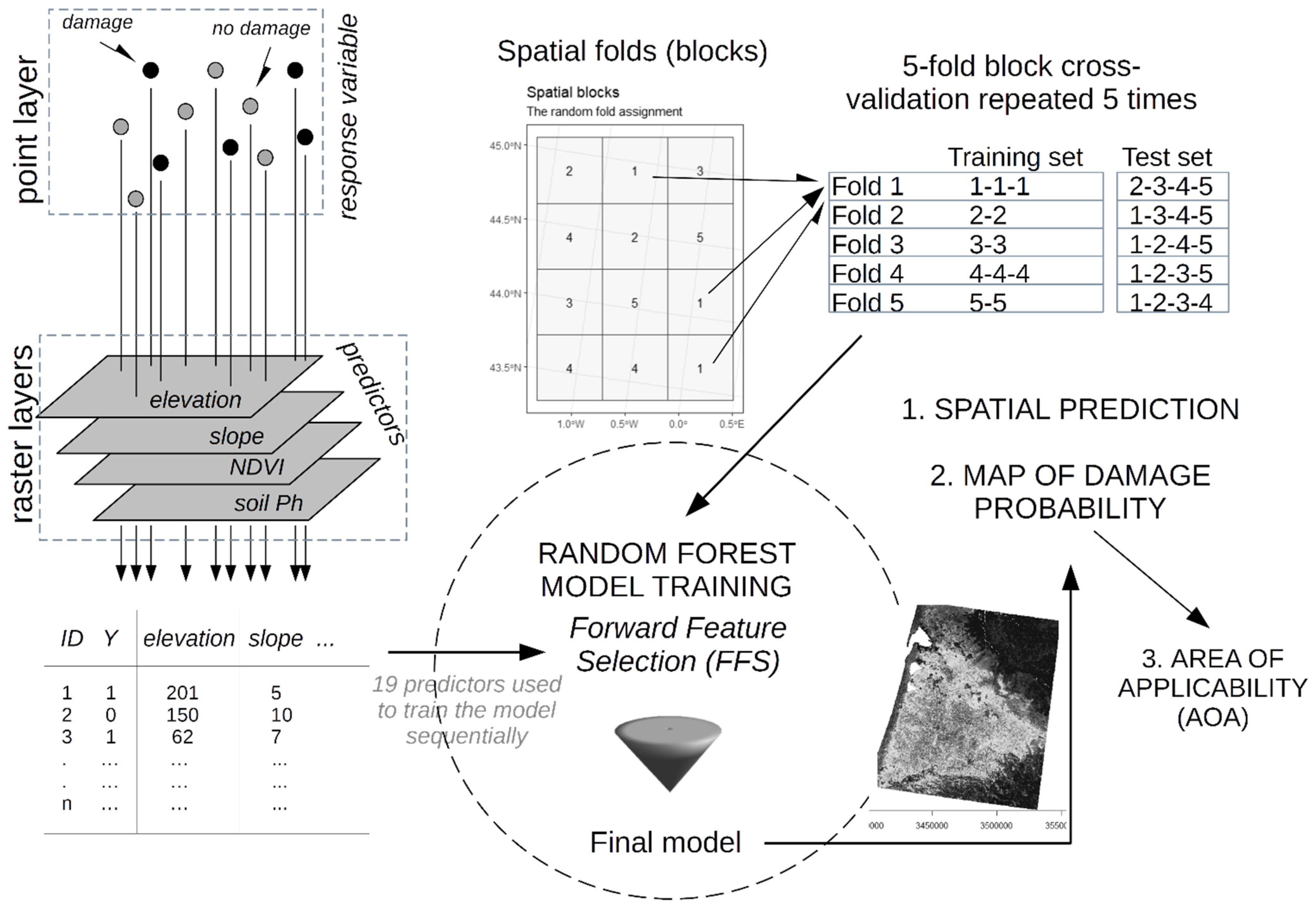
2.4. Model Training and Evaluation

2.4.1. Data Pre-Processing and Model Training

The caret R package was used for model training [53,54]. We applied RF to solve the classification problem. The RF model is a modern decision tree based ensemble learning technique that can be used for classification and regression [55,56]. The method builds multiple independent trees using bagging and averaging their results [57]. This is known to increase model stability and accuracy. The RF allows hyperparameters tuning such as mtry, which is a random sample of the m predictors, to split at in each node, and min_n, which is a minimum terminal node size. The number of trees can be tuned but it is also recommended to set it to a sufficiently and computationally effective number [58]. In the present project, the number of trees was set to 500.
Before the training process, highly correlated (|r| > 0.75) variables were excluded to avoid multicollinearity between independent variables. When two variables were correlated, the program analyzed how they were correlated with other variables and excluded the one which had a higher level of correlation with them. In order to avoid over-fitting, instead of random cross-validation, we applied spatial block cross-validation [59,60], the procedure that takes into account the spatial domain of the data structure. For that task we used the blockCV [60] and the caretSDM [61] R package. Five-fold block cross-validation repeated five times was applied (Figure 3). Such an approach is based on a Leave-Location-Out (LLO) Cross-Validation principle [62]. Ignoring the spatial scale and selecting the training and test set randomly from the entire study area could lead to over-fitting because the training and test points were sampled from the same area [62,63]. In other words, the random selection of the test points does not guarantee independence from training points due to spatial autocorrelation [63].
Before the training procedure, the data set was split into training and test sets (60 and 40%, respectively). During the model training stage, we used forward feature selection (FFS) to automatically identify and remove variables that could lead to over-fitting [62]. This method was implemented in the CAST R package [62].

2.4.2. Model Evaluation

For model evaluation, we used the following metrics: (1) the area under the receiver operating characteristics curve (ROC AUC); (2) accuracy; (3) variable importance (VI); and (4) accumulation local effects (ALE) plots.
Accuracy is the ratio between the correct predictions and all predictions. The ROC curve computes the sensitivity (i.e., recall, true positive class divided by the total number of positive results) and specificity (true negative divided by the sum of false positives and true negatives) over a continuum of different event thresholds [64,65]. The ROC AUC is a measure of the probability of correctly identifying a positive signal (response 1 in binary classification) above the noise [66]. In the present study, we adopted the common threshold level of probability used to discriminate between a positive and negative class of 0.5. The classes of ROC AUC were defined as follows: AUC = 0.5 (random discrimination between binary classes), AUC = (0.5, 0.7] (weak discrimination), AUC = (0.7, 0.8] (acceptable discrimination), AUC = (0.8, 0.9] (excellent discrimination), AUC = (0.9, 1.0) (outstanding discrimination), and AUC = 1.0 (perfect discrimination between classes) [67,68]. Variable importance (VI) was calculated to evaluate each predictor’s contribution to the model. VI is a metric that describes accuracy and relies on the information in each predictor [69]. A higher VI indicates that a predictor has a stronger impact on the response variable and accumulation local effects (ALE) is a model diagnostic tool that explains the average influence of the features on the prediction [70]. It works in a similar way to partial dependence plots (PDP), but it is considered a better measure because it is less sensitive to correlations between predictors.

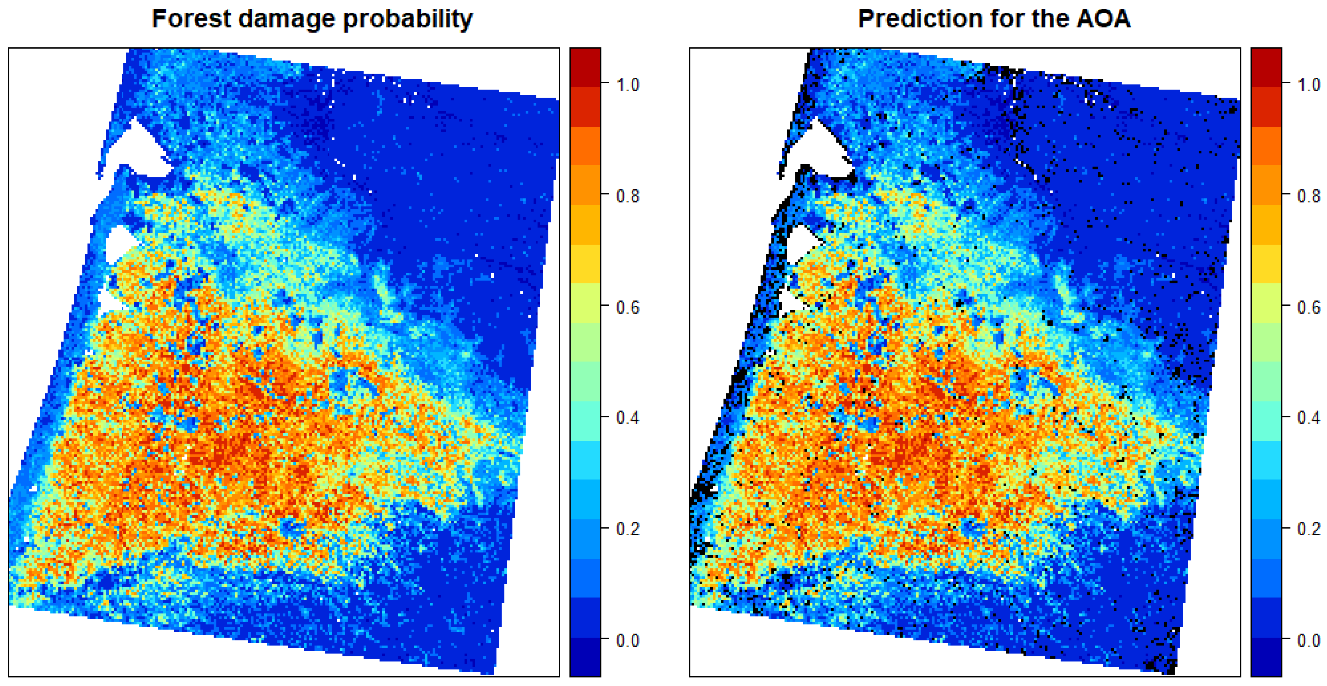
2.4.3. Prediction and Probability Maps
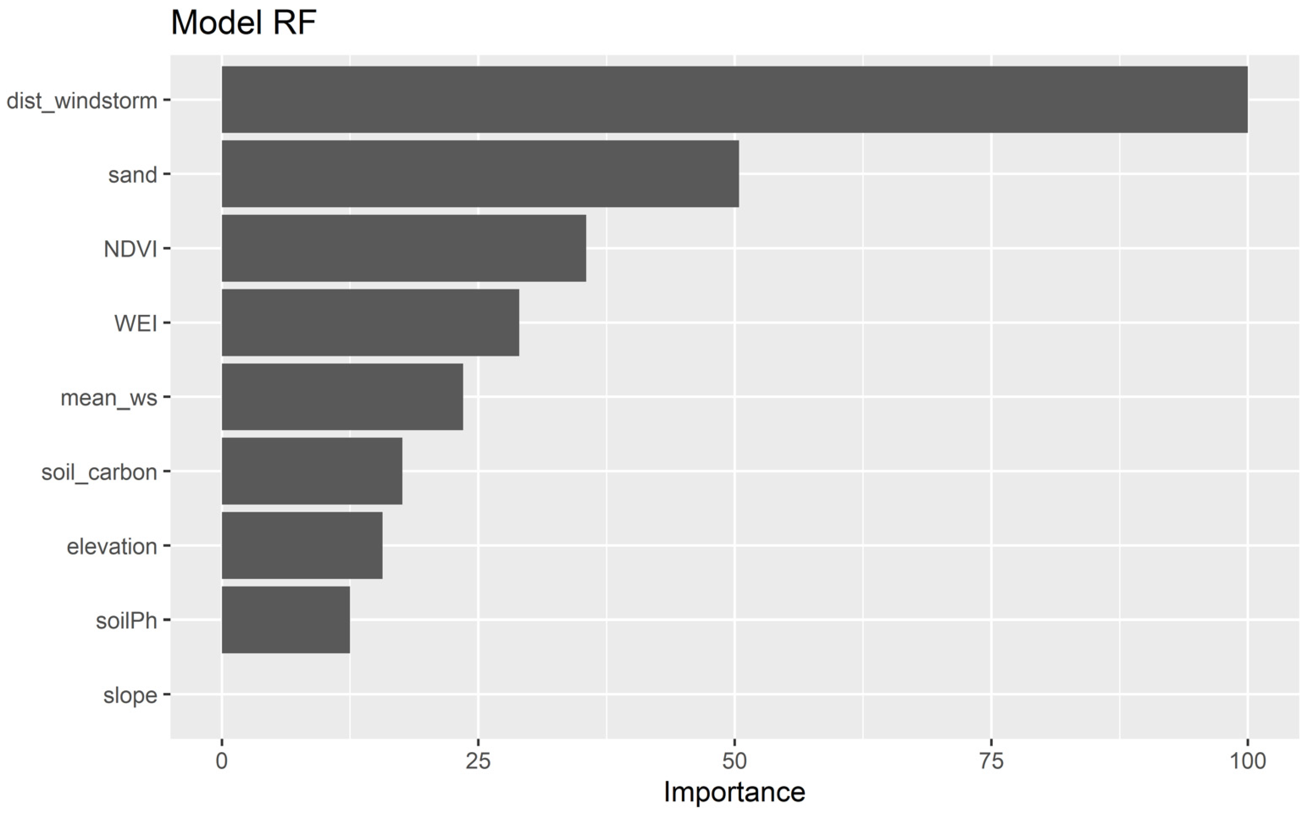
Spatial prediction was performed using the raster::predict function in R. To speed up the computation time, all rasters were aggregated to 100 m of spatial resolution. We applied the Area of Applicability (AOA) technique to test whether the RF model performs equally well across the entire study area [71]. AOA is the area where the model can learn relationships between variables based on the training data, and where the estimated cross-validation performance holds [71].

3. Results

Our results indicated that the RF model correctly discriminated between binary classes (damage vs. no damage) and can be a useful tool in forest damage modelling and prediction. From nineteen potential predictors, nine were selected during the FFS procedure as important and did not lead to model over-fitting. The four most important predictors were the distance from the windstorm trajectory, sand fraction content, NDVI, and WEI (Figure 4). Unexpectedly, the January mean wind speed (mean_ws) was less important, as were the other abiotic predictors (soil carbon content, elevation, soil pH, and slope). The model performance of the optimal model measured by ROC_AUC was 0.895, and the accuracy was 0.82. The model was trained on 7275 observations. After applying the model to the test set (n = 4844) the ROC_AUC was 0.899, and the accuracy reached 0.837 (balanced accuracy = 0.835).
In terms of the individual effect of each predictor, the four most important features (distance from the windstorm track, sand content, NDVI, and WEI) had a positive effect; with their increasing values, the damage probability also increased (Figure 5). The probability of damage increased at a distance between 75 and 150 km from the windstorm trajectory (dist_windstorm). The soil sand fraction content had a positive impact on forest damage when reaching between 35 and 60%. In addition, the forest damage probability increased when the WEI increased over 0.95 and remained almost constant over WEI 1.05. The values of NDVI over 0.5 also positively impacted the forest damage probability. Five other variables (less important), such as mean wind speed in January, soil carbon content, elevation, soil pH, and slope, had different effects on damage probability (only partially positive). The mean wind speed had a positive effect when reaching up to 2.0 ms−1 and for 2.75–3.25 ms−1. A higher mean wind speed did not affect the damage probability. The soil carbon content, which is a measure of soil fertility and edaphic conditions of forest growth, had a positive impact up to 4 units. After that point, the level of damage probability decreased and remained almost constant for soil carbon over 6 units. The terrain elevation had positive impact on the damage probability up to ca. 60 m asl. Soil pH, which is also a measure of soil fertility, has a minor positive impact on forest damage probability up to ca. 6.2 units. The slope had a negligible effect on forest vulnerability to damage (Figure 5).
After applying the RF model to the entire AOI, we were able to obtain maps of damage probability. Clusters of high forest damage probability were computed primarily for the central part of the study area, some distance from the Atlantic Ocean coastline, and the windstorm trajectory, which was North of the area (Figure 6). The Area of Applicability (AOA) confirmed the RF model could be successfully applied to the entire area, with some minor areas of model inapplicability along the coastline.

4. Discussion

We found a greater forest damage probability with increasing distance from the windstorm track, up to 150 km. A similar tendency was reported in New England (USA) forests, which were impacted by hurricanes in 1944 [72]. It was found that the sites that experienced higher rates of damage were located further east of the storm track and closer to the area of maximum estimated wind speed [73]. This is an important, and yet understudied, finding because it allows for the approximate evaluation of windstorm damage and probability of damage based on predicted windstorm trajectory, even in near real-time projections. Other studies found the highest importance of forest biomass (volume in m3) and tree age predictors [9]. However, in many instances, forest feature data were not available or not up to date, thus favoring the application of other predictors that were easier to access and implement. We found a higher damage probability with increasing NDVI. High NDVI values can be interpreted as mature forests with a better health condition [74]. Some studies have found weak correlations between NDVI and forest biomass [74]. That agrees with our previous results, where the tree biomass was found to be the most important predictor [9].
In the past, several approaches were tested to isolate the best predictive models of forest damage triggered by strong winds [11,68,74]. However, the results differed in the level of model predictive power [68,75,76,77], and in most cases our RF model outperformed other models. We were able to reach a higher precision of the RF model, which was 0.899 (ROC AUC) and 0.837 (accuracy) after applying the model to the test set. Fridman and Valinger [75] obtained an accuracy of 0.8 using tree, stand, and site characteristics from study plots in Sweden as an input data for the logistic regression model. Schindler et al. [76] analyzed the damage caused in Germany by the windstorm Lothar in 1999. After using the logistic regression modelling the model precision measured by ROC AUC reached 0.79. The highest probability of damage was predicted for coniferous forest stands growing on acidic, fresh, and moist soils [76]. Klaus et al. [77] obtained an accuracy level of 0.7, based on GLM modelling of damage caused by the windstorm Kyrill in Germany in 2007. They highlighted the sensitivity of forest stands to windthrow as the effect of a high proportion of coniferous trees, a complex topography, and immature soils. Suvanto et al. [68] obtained ROC AUC close to 0.73 for damage probability in Finland and were able to demonstrate a level of precision for a large database over the entire country. Pawlik and Harrison [9] presented the RF model, of which the precision measured by ROC AUC was 0.71. They analyzed data for the Sudety region in Poland and found that forest volume and tree age were the most important predictors. There might be several reasons behind the differences in the models’ precision obtained by various authors in comparison to the results presented here. The most likely are: (1) different machine learning methods applied (here RF which is a decision tree-based method); (2) a different set and number of potential predictors (19 predictors reduced to 9); (3) application of spatial block cross-validation; (4) use of the forward feature selection.
For the same study area, Kamimura et al. [10] used tree census data for the evaluation and modelling of the damage caused by windstorm Klaus. They used data from 235 plots, collected in 2007 and 2008 by the French foresters during national inventories. Additionally, trees damaged by windstorm Klaus were identified. This unique database consisted of several tree features, including height, diameter at breast height, and tree age. With as many as 25 predictors, Kamimura et al. [10] were able to train the logistic regression model, which reached AUC = 0.791 and an accuracy of 0.717. Although such a level of accuracy is acceptable, it can also indicate that the data set used in their study was too small, or that the modelling based on individual tree features was not able to capture any significant signal from the data. Despite the statistical modelling of windstorm Klaus, the authors had some difficulties finding the optimal logistic regression model. Nevertheless, they were able to isolate the most important predictors, which were soil type and the year of forest establishment [10]. In our study, we considered five soil features (Table 1) that we thought could support a better explanation of the spatial structure of the forest damage. Soil clay and sand fraction content is critical for the development and architecture of the root systems, which are important for tree stability during high wind events [10,20]. The root systems are weakly developed in soils that are immature, too shallow, or containing too high content of gravels. In such soils, root systems may not provide secure anchorage in the ground or overall stability. Additionally, hydromorphic soils (saturated or waterlogged soils) can prevent trees from developing deep root systems. Maritime pine trees were found to have less anchorage in wet soils [78]. We found that the damage probability was positively influenced by a higher sand content. The soil type in the area of investigation primarily contained podzols of more than 55 cm in depth [10]. Sandy soils, such as podzols, cannot secure good tree stability. Further, data on Sitka spruce (Picea sitchensis) collected during tree-pulling experiments in the UK suggested better anchorage on peat than on gleyed mineral soils [79]. While applying the tree-pulling experiments in the same study area in southwest France, Cucchi et al. [37] found evidence of higher stability (better anchorage) for maritime pine on dry podzols with a deeper groundwater table, and a broken or absent hard pan. However, such conditions frequently cause stem failure. In addition, we found important, albeit minor, impact of soil pH and carbon content on the level of forest damage probability. Both indicators provide information on soil fertility and quality. It was also found that the risk of windstorm damage increased with a growing deterioration of the humus form and higher soil acidity (i.e., lower soil pH) [80]. This was partly supported by our study, as we found that the forest stands growing on alkaline soils had a very low damage probability.
We concluded that the WEI increased the probability of damage. When >1.0, this dimensionless index indicates areas exposed to wind impact. The RF model correctly discriminated between exposed (>1.0) and unexposed (<1.0) places where the increase in damage probability was always over zero (Figure 4). The study area was rather flat; however, at a resolution of 25 m the WEI algorithm applied in SAGA GIS was able to find significant differences in the terrain exposure to wind. This is in line with our previous results [9]. Rapid damage propagation can be expected close to the coastline, irrespective of tree features, as pointed out by Kamimura et al. [10]; however, we did not find the distance from the coastline as an important predictor. Although difficult to measure, wind speed is a key predictor in forest damage modelling [9,81]. Of the three wind-related predictors used in our study (Table 1), only mean January wind speed was important, but not as significant as expected. According to our results, the forest damage probability increased at short intervals when the mean wind speed was >0.25 ms−1, and between 2.75 and 3.25 ms−1. In the Sudety Mountains, SW Poland, it was found that the forest damage probability increased proportionally to the mean June wind speed, between 3 and 6 m s−1 [9]. Several historical studies reviewed by Gardiner [12] indicated an increasing damage probability with increasing wind speed. In Finland, it was found that the relationship between wind gust speed and volume of forest damage followed a power function, with a power of approximately 10 [81]. However, there is a common agreement that such a relationship is highly dependent on regional wind conditions and tree features (tree species, height, age, and health status). Due to the managed nature of the forest and past forest management in our AOI, we cannot assume that maritime pines had natural resistance to wind impact [10]. The raster layer containing wind speed data from the Windstorm Information Service (Table 1) indicated rapid wind speed decline, from 47 to 27 m s−1, with increasing distance from the coastline, 20 to 50 km, particularly in the northern part of the region (Figure S1, Supplementary Materials). The highest damage density for the class of damage ≥ 0.7 was between 15 and 50 km from the coastline. However, we presume that most of the trees in some heavily impacted forest inspectorates were damaged by wind speeds below the level of 30 m s−1 (which is still high). Past reports suggest that even lower, but sustained, wind speeds and gusts can cause widespread damage in forests [12].
The biggest limitation of our modelling approach was the lack of detailed information on tree and forest properties before and after the event. One of the ways to overcome that limitation was to use vegetation indices based on satellite images, i.e., NDVI. Data on individual tree features are difficult to obtain, especially after windstorm events, when all trees in managed forests are subject to sanitary removal for safety and economic reasons. Therefore, we focused on forest characteristics that are easily accessible via the Internet and are also high-quality products (in terms of classification and spatial resolution precision) based on the reanalysis of satellite images. Furthermore, in some cases, building a model using information on individual tree characteristics cannot provide satisfactory prediction accuracy [10]. Considering these advantages and limitations, this study used general information about forest conditions, namely NDVI and LAI. Our results suggest that only NDVI can accommodate a strong signal of forest damage in specific conditions of the maritime pine forest.

5. Conclusions

Windstorm Klaus was among the most devastating extreme climate events in the history of European meteorological records. The windstorm left a significant imprint in forest stands, particularly in France, as well as high financial losses and many casualties. After applying machine learning techniques, we were able to identify some underlying relationships that may help improve forest damage risk management due to strong wind events. This can be a valuable starting point for other analyses and planning in regions with similar natural conditions as our study area in southwest France affected by windstorm Klaus. We were able to map the probability of forest damage using the RF method. RF can be used for a quick evaluation of the most important features behind the high rate of forest damage during extra-tropical cyclones. These events may occur more frequently in the near future, and for that reason, their thorough understanding is a key prerequisite for better planning. This can also ensure a basic level of warning system functionality. In the present study, we found, for the first time, that the distance from the windstorm track, wind exposure of the terrain, and soil properties, should always be considered as important predictors. When detailed information on forest structure and features is not directly accessible, NDVI can be used as a good approximation of forest conditions and history. The information can be easily obtained using various web services. Additionally, prediction maps offer a general overview of forest damage probability in geographic regions and will aid future steps in forest management, ecology, and geomorphology.

Supplementary Materials

The following supporting information can be downloaded at: https://www.mdpi.com/article/10.3390/f13121991/s1, Figure S1: Density function of the distance from the Atlantic coastline displayed for the two classes of the binary response variable. Abbreviations: dam—damage class, no_dam—places with no damage class; Table S1: Basic properties of the damage classes adopted in the study.

Author Contributions

Conceptualization, Ł.P.; methodology, Ł.P.; validation, Ł.P.; formal analysis, Ł.P. and J.G.; investigation, Ł.P. and J.G.; data curation, Ł.P.; writing—original draft preparation, Ł.P. and J.G.; writing—review and editing, Ł.P. and J.G.; visualization, Ł.P., J.G. and Ł.Z.; supervision, Ł.P.; project administration, Ł.P.; funding acquisition, Ł.P. All authors have read and agreed to the published version of the manuscript.

Funding

This study was supported by the Polish National Center—Narodowe Centrum Nauki (grant no 2019/35/O/ST10/00032).

Data Availability Statement

Data will be shared on request to the corresponding author.

Acknowledgments

Two anonymous reviewers are thanked for their insightful comments and suggestions that allowed us to improve the final version of the manuscript. In addition, we want to thank Lukasz Longosz for proofreading the final draft of the manuscript.

Conflicts of Interest

The authors declare no conflict of interest.

References

  1. Walz, M.A.; Kruschke, T.; Rust, H.W.; Ulbrich, U.; Leckebusch, G.C. Quantifying the extremity of windstorms for regions featuring infrequent events. Atmos. Sci. Lett. 2017, 18, 315–322. [Google Scholar] [CrossRef]
  2. Romeiro, J.M.N.; Eid, T.; Antón-Fernández, C.; Kangas, A.; Trømborg, E. Natural disturbances risks in European Boreal and Temperate forests and their links to climate change—A review of modelling approaches. For. Ecol. Manag. 2022, 509, 120071. [Google Scholar] [CrossRef]
  3. Spinoni, J.; Formetta, G.; Mentaschi, L.; Forzieri, G.; Feyen, L. Global Warming and Windstorm Impacts in the EU; JRC Technical Report; EUR 29960 EN; Publications Office of the European Union: Luxembourg, 2020. [Google Scholar] [CrossRef]
  4. Ranson, M.; Kousky, C.; Ruth, M.; Jantarasami, L.; Crimmins, A.; Tarquinio, L. Tropical and extratropical cyclone damages under climate change. Clim. Chang. 2014, 127, 227–241. [Google Scholar] [CrossRef] [Green Version]
  5. Senf, C.; Seidl, R. Storm and fire disturbances in Europe: Distribution and trends. Glob. Chang. Biol. 2021, 27, 3605–3619. [Google Scholar] [CrossRef]
  6. Masson-Delmotte, V.; Zhai, P.; Pirani, A.; Connors, S.L.; Péan, C.; Berger, S.; Caud, N.; Chen, Y.; Goldfarb, L.; Gomis, M.I.; et al. (Eds.) IPCC Climate Change 2021: The Physical Science Basis. In Contribution of Working Group I to the Sixth Assessment Report of the Intergovernmental Panel on Climate Change; Cambridge University Press: Cambridge, UK, 2021; Available online: https://www.ipcc.ch/report/ar6/wg1/ (accessed on 1 October 2022).
  7. Jahani, A.; Saffariha, M. modelling of trees failure under windstorm in harvested Hercynian forests using machine learning techniques. Sci. Rep. 2021, 11, 1124. [Google Scholar] [CrossRef] [PubMed]
  8. Pettit, J.L.; Pettit, J.M.; Janda, P.; Rydval, M.; Čada, V.; Schurman, J.S.; Nagel, T.A.; Bače, R.; Saulnier, M.; Hofmeister, J.; et al. Both cyclone-induced and convective storms drive disturbance patterns in European primary beech forests. J. Geophys. Res. Atmos. 2021, 126, e2020JD033929. [Google Scholar] [CrossRef]
  9. Pawlik, Ł.; Harrison, S.P. modelling and prediction of wind damage in forest ecosystems of the Sudety Mountains, SW Poland. Sci. Total Environ. 2022, 815, 151972. [Google Scholar] [CrossRef] [PubMed]
  10. Kamimura, K.; Gardiner, B.; Dupont, S.; Guyon, D.; Meredieu, C. Mechanistic and statistical approaches to predicting wind damage to individual maritime pine (Pinus pinaster) trees in forests. Can. J. For. Res. 2016, 46, 1. [Google Scholar] [CrossRef]
  11. Hart, E.; Sim, K.; Kamimura, K.; Meredieu, C.; Guyon, D.; Gardiner, B. Use of machine learning techniques to model wind damage to forests. Agric. For. Meteorol. 2019, 265, 16–29. [Google Scholar] [CrossRef]
  12. Gardiner, B. Wind damage to forets and trees: A review with an emphasis on planted and managed forests. J. For. Res. 2021, 26, 248–266. [Google Scholar] [CrossRef]
  13. Gardiner, B.; Byrne, K.; Hale, S.; Kamimura, K.; Mitchell, S.J.; Peltola, H.; Ruel, J.C. A review of mechanistic modelling of wind damage risk to forests. Forestry 2008, 81, 447–463. [Google Scholar] [CrossRef] [Green Version]
  14. Lopes, A.M.G. WindStation—A software for the simulation of atmospheric flows over complex topography. Environ. Model. Softw. 2003, 18, 81–96. [Google Scholar] [CrossRef]
  15. Hale, S.; Gardiner, B.; Peace, A.; Nicoll, B.; Taylor, P.; Pizzirani, S. Comparison and validation of three versions of a forest wind risk model. Environ. Model. Softw. 2015, 68, 27–41. [Google Scholar] [CrossRef] [Green Version]
  16. Peltola, H.; Kellomäki, S.; Vaisanen, H.; Ikonene, V.-P. A mechanistic model for assessing the risk of wind and snow damage to single trees and stands of Scots pine, Norway spruce, and birch. Can. J. For. Res. 1999, 29, 647–661. [Google Scholar] [CrossRef]
  17. Gardiner, G.; Suárez, J.; Achim, A.; Hale, S.; Nicoll, B. ForestGALES: A PC-Based Wind Risk Model for British Forests; User’s Guide Version 2.0; Forestry Commission: Edinburgh, UK, 2004. [Google Scholar]
  18. Everham, E.M.; Brokaw, N.V. Forest damage and recovery from catastrophic wind. Bot. Rev. 1996, 62, 113–185. [Google Scholar] [CrossRef]
  19. Mitchell, S. Wind as a natural disturbance agent in forests: A synthesis. Forestry 2013, 86, 147–157. [Google Scholar] [CrossRef] [Green Version]
  20. Gardiner, B.; Schuck, A.; Schelhaas, M.-J.; Orazio, C.; Blennow, K.; Nicoll, B. Living with Storm Damage to Forests: What Science Can Tell Us; European Forest Institute: Joensuu, Finland, 2013. [Google Scholar]
  21. Gregow, H.; Laaksonen, A.; Alper, M.E. Increasing large scale windstorm damage in western, central and northern European forests, 1951–2010. Sci. Rep. 2017, 7, 46397. [Google Scholar] [CrossRef] [PubMed] [Green Version]
  22. Negrón-Juárez, R.I.; Jenkins, H.S.; Raupp, C.F.M.; Riley, W.J.; Kueppers, L.M.; Magnabosco Marra, D.; Ribeiro, G.H.P.M.; Monteiro, M.T.F.; Candido, L.A.; Chambers, J.Q.; et al. Windthrow variability in Central Amazonia. Atmosphere 2017, 8, 28. [Google Scholar] [CrossRef] [Green Version]
  23. Schelhaas, M.-J.; Nabuurs, G.-J.; Schuck, A. Natural disturbances in the European forests in the 19th and 20th centuries. Glob. Chang. Biol. 2003, 9, 1620–1633. [Google Scholar] [CrossRef]
  24. Seidl, R.; Schelhaas, M.-J.; Lexer, M.J. Unraveling the drivers of intensifying forest disturbance regimes in Europe. Glob. Chang. Biol. 2011, 17, 2842–2852. [Google Scholar] [CrossRef]
  25. Dacre, H.F.; Pinto, J.G. Serial clustering of extratropical cyclones: A review of where, when and why it occurs. NPJ Clim. Atmos. Sci. 2020, 3, 48. [Google Scholar] [CrossRef]
  26. Caurla, S.; Garcia, S.; Niedzwiedz, A. Store or export? An economic evaluation of financial compensation to forest sector after windstorm. The case of Hurricane Klaus. For. Policy Econ. 2015, 61, 30–38. [Google Scholar] [CrossRef]
  27. Liberato, M.L.R.; Pinto, J.G.; Trigo, I.F.; Trigo, R.M. Klaus—An exceptional winter storm over northern Iberia and southern France. Weather 2011, 66, 330–334. [Google Scholar] [CrossRef] [Green Version]
  28. Aon-Benfield, Annual Global Climate and Catastrophe Report IF 2009. 2010. Available online: https://www.aon.com/attachments/reinsurance/200912_ab_if_impact_forecasting_2009_report.pdf (accessed on 1 October 2022).
  29. Tuppen, J.N.; Bachrach, B.S.; Higonnet, P.L.-R.; Flower, J.E.; Popkin, J.D.; Wright, G.; Bisson, T.N.; Shennan, J.H.; Fournier, G.; Elkins, T.H.; et al. “France”. Encyclopedia Britannica. 3 November 2021. Available online: https://www.britannica.com/place/France (accessed on 1 October 2022).
  30. Forzieri, G.; Pecchi, M.; Girardello, M.; Mauri, A.; Klaus, M.; Nikolov, C.; Rüetschi, M.; Gardiner, B.; Tomaštík, J.; Small, D.; et al. A spatially explicit database of wind disturbances in European forests over the period 2000–2018. Earth Syst. Sci. Data 2020, 12, 257–276. [Google Scholar] [CrossRef] [Green Version]
  31. Beck, H.E.; Zimmermann, N.E.; McVicar, T.R.; Vergopolan, N.; Berg, A.; Wood, E.F. Present and future Köppen-Geiger climate classification maps at 1-km resolution. Sci. Data 2018, 5, 180214. [Google Scholar] [CrossRef] [Green Version]
  32. NOAA GSOD, National Oceanic and Atmospheric Administration, Global Summary of the Day, U.S. Department of Commerce. 2021. Available online: https://www7.ncdc.noaa.gov/CDO/cdoselect.cmd?datasetabbv=GSOD (accessed on 6 November 2021).
  33. Alison, C. (Ed.) Michelin Green Guide: French Atlantic Coast; Michelin Apa Publications: London, UK, 2010; Volume 8, pp. 258–263. ISBN 1-906261-79-2. [Google Scholar]
  34. Hansen, M.C.; Potapov, P.V.; Moore, R.; Hancher, M.; Turubanova, S.A.; Tyukavina, A.; Thau, D.; Stehman, S.V.; Goetz, S.J.; Loveland, T.R.; et al. High-resolution global maps of 21st-century forest cover change. Science 2013, 342, 850–853. [Google Scholar] [CrossRef] [PubMed] [Green Version]
  35. Cucchi, V.; Bert, D. Wind-firmness in Pinus pinaster Aït. Stands in Southwest France: Influence of stand density, fertilisation and breeding in two experimental stands damaged during the 1999 storm. Ann. For. Sci. 2003, 60, 209–226. [Google Scholar] [CrossRef] [Green Version]
  36. Cucchi, V.; Meredieu, C.; Stokes, A.; Barthier, S.; Bert, D.; Najar, M.; Denis, A.; Lastennet, R. Root anchorage of inner and edge trees in stands of Maritime pine (Pinus pinaster Ait.) growing in different podzolic soil conditions. Trees 2004, 18, 460–466. [Google Scholar] [CrossRef]
  37. Tuck, S.L.; Phillips, H.R.P.; Hintzen, R.E.; Scharlemann, J.P.W.; Purvis, A.; Hudson, L.N. MODISTools—Downloading and processing MODIS remotely sensed data in R. Ecol. Evol. 2014, 4, 4658–4668. [Google Scholar] [CrossRef]
  38. Hijmans, R.J. Raster: Geographic Data Analysis and Modelling. R Package Version 3.3-13. 2020. Available online: https://CRAN.R-project.org/package=raster (accessed on 1 October 2022).
  39. Horn, B.K.P. Hill shading and the reflectance map. Proc. IEEE 1981, 69, 14–47. [Google Scholar] [CrossRef] [Green Version]
  40. Evans, J.S. _spatialEco_. R Package Version 1.3-6. 2021. Available online: https://github.com/jeffreyevans/spatialEco (accessed on 1 October 2022).
  41. Conrad, O.; Bechtel, B.; Bock, M.; Dietrich, H.; Fischer, E.; Gerlitz, L.; Wehberg, J.; Wichmann, V.; Böhner, J. System for Automated Geoscientific Analyses (SAGA) v. 2.1.4. Geosci. Model Dev. 2015, 8, 1991–2007. [Google Scholar] [CrossRef] [Green Version]
  42. Moore, I.D.; Grayson, R.B.; Ladson, A.R. Digital terrain modelling: A review of hydrological, geomorphological, and biological applications. Hydrol. Processes 1991, 5, 3–30. [Google Scholar] [CrossRef]
  43. Dyderski, M.K.; Pawlik, Ł. Drivers of forest aboveground biomass and its increments in the Tatra Mountains after 15 years. Catena 2021, 205, 105468. [Google Scholar] [CrossRef]
  44. Hengl, T.; Mendes de Jesus, J.; Heuvelink, G.B.M.; Ruiperez Gonzalez, M.; Kilibarda, M.; Blagotić, A.; Shangguan, W.; Wright, M.N.; Geng, X.; Bauer-Marschallinger, B.; et al. SoilGrids250m: Global gridded soil information based on machine learning. PLoS ONE 2017, 12, e0169748. [Google Scholar] [CrossRef] [PubMed] [Green Version]
  45. Watson, D.J. The estimation of leaf area in field crops. J. Agric. Sci. 1937, 27, 474–483. [Google Scholar] [CrossRef]
  46. Clark, J.; Bobbe, T. Using remote sensing to map and monitor fire damage in forest ecosystems. In Understanding Forest Disturbance and Spatial Pattern; Michael, A.W., Steven, E.F., Eds.; Remote Sensing and GIS Approaches; Taylor and Francis: New York, NY, USA, 2007; pp. 113–131. [Google Scholar]
  47. QGIS.org, QGIS Geographic Information System. QGIS Association. 2021. Available online: https://www.qgis.org (accessed on 1 October 2022).
  48. Hodges, K.I. Feature tracking on the unit sphere. Mon. Weather Rev. 1995, 123, 3458–3465. [Google Scholar] [CrossRef]
  49. Whitelaw, A.; Shaffrey, L.; Hodges, K. WISC Storm Tracks Description. Copernicus Climate Change Service. 2017. Available online: https://wisc.climate.copernicus.eu/wisc/documents/shared/C3S_WISC_Storm%20Track_Description_v1.0.pdf (accessed on 1 October 2022).
  50. Pebesma, E. Simple Features for R: Standardized Support for Spatial Vector Data. R J. 2018, 10, 439–446. [Google Scholar] [CrossRef] [Green Version]
  51. Bivand, R.; Rundel, C. rgeos: Interface to Geometry Engine—Open Source (‘GEOS’). R Package Version 0.5-7. 2021. Available online: https://CRAN.R-project.org/package=rgeos (accessed on 1 October 2022).
  52. Bonannella, C.; Hengl, T.; Heisig, J.; Parent, L.; Wright, M.N.; Herold, M.; de Bruin, S. Forest tree species distribution for Europe 2000-2020: Mapping potential and realized distributions using spatiotemporal machine learning. PeerJ 2022, 10, e13728. [Google Scholar] [CrossRef]
  53. Kuhn, M. Building predictive models in R using the caret package. J. Stat. Softw. 2008, 28, 1–26. [Google Scholar] [CrossRef]
  54. Kuhn, M. Caret: Classification and Regression Training. R Package Version 6.0-86. 2020. Available online: https://CRAN.R-project.org/package=caret (accessed on 1 October 2022).
  55. Breiman, L. Random forests. Mach. Learn. 2001, 45, 5–32. [Google Scholar] [CrossRef] [Green Version]
  56. Probst, P.; Boulesteix, A.-L. To tune or not to tune the number of trees in random forest? arXiv 2017, arXiv:1705.05654. [Google Scholar]
  57. Lesmeister, C.; Chinnamgari, S.K. Advanced Machine Learning with R; Packt: Birmingham, UK; Mumbai, India, 2019; 649p. [Google Scholar]
  58. Hengl, T.; Nussbaum, M.; Wright, M.N.; Heuvelink, G.B.M.; Gräler, B. Random forest as a generic framework for predictive modeling of spatial and spatio-temporal variables. PeerJ 2018, 6, e5518. [Google Scholar] [CrossRef] [Green Version]
  59. Roberts, D.R.; Bahn, V.; Ciuti, S.; Boyce, M.S.; Elith, J.; Guillera-Arroita, G.; Hauenstein, S.; Lahoz-Monfort, J.J.; Schröder, B.; Thuiller, W.; et al. Cross-validation strategies for data with temporal, spatial, hierarchical, or phylogenetic structure. Ecography 2017, 40, 913–929. [Google Scholar] [CrossRef] [Green Version]
  60. Valavi, R.; Elith, J.; Lahoz-Monfort, J. BlockCV: An R package for generating spatially or environmentally separated folds for k-fold cross-validation of species distribution models. Methods Ecol. Evol. 2019, 10, 225–232. [Google Scholar] [CrossRef] [Green Version]
  61. Corrêa, P. caretSDM—Species Distribution Models Using Caret, v.0.2.0. 2021. Available online: https://github.com/correapvf/caretSDM (accessed on 1 October 2022).
  62. Meyer, H.; Reudenbach, C.; Hengl, T.; Katurji, M.; Nauss, T. Improving performance of spatio-temporal machine learning models using forward feature selection and target-oriented validation. Environ. Model. Softw. 2018, 101, 1–9. [Google Scholar] [CrossRef]
  63. Ploton, P.; Mortier, F.; Réjou-Méchain, M.; Barbier, N.; Picard, N.; Rossi, V.; Dormann, C.; Cornu, G.; Viennois, G.; Bayol, N.; et al. Spatial validation reveals poor predictive performance of large-scale ecological mapping models. Nat. Commun. 2020, 11, 4540. [Google Scholar] [CrossRef] [PubMed]
  64. Fawcett, T. An introduction to ROC analysis. Pattern Recognit. Lett. 2006, 27, 861–874. [Google Scholar] [CrossRef]
  65. Kuhn, M.; Silge, J. Tidy Modelling with R. 2020. Available online: https://www.tmwr.org/ (accessed on 1 October 2022).
  66. Hanley, J.A.; McNeil, B.J. The meaning and use of the area under a receiver operating characteristic (ROC) curve. Radiology 1982, 143, 29–36. [Google Scholar] [CrossRef] [PubMed] [Green Version]
  67. Hosmer, D.W.; Lemeshow, S.; Strudivant, R.X. Applied Logistic Regression, 3rd ed.; John Wiley and Sons: New York, NY, USA, 2013. [Google Scholar]
  68. Suvanto, S.; Peltoniemi, M.; Tuominen, S.; Strandström, M.; Lehtonen, A. High-resolution mapping of forest vulnerability to wind for disturbance-aware forestry. For. Ecol. Manag. 2019, 453, 117619. [Google Scholar] [CrossRef]
  69. Fisher, A.; Rudin, C.; Dominici, F. All models are wrong, but many are useful: Learning a variable’s importance by studying an entire class of prediction models simultaneously. J. Mach. Learn. Res. 2019, 20, 1–81. [Google Scholar]
  70. Molnar, C. Interpretable Machine Learning. A Guide for Making Black Box Models Explainable. 2020. Available online: https://christophm.github.io/interpretable-ml-book/ (accessed on 1 October 2022).
  71. Meyer, H.; Pebesma, E. Predicting into unknown space? Estimating the area of applicability of spatial prediction models. Methods Ecol. Evol. 2021, 12, 1620–1633. [Google Scholar] [CrossRef]
  72. Busby, P.E.; Motzkin, G.; Boose, E.R. Landscape-level variation in forest response to hurricane disturbance across a storm track. Can. J. For. Res. 2008, 38, 2942–2950. [Google Scholar] [CrossRef] [Green Version]
  73. Ogaya, R.; Barbeta, A.; Başnou, C.; Penuelas, J. Satellite data as indicators of tree biomass growth and forest dieback in a Mediterranean holm oak forest. Ann. For. Sci. 2015, 72, 135–144. [Google Scholar] [CrossRef] [Green Version]
  74. Hanewinkel, M.; Zhou, W.; Schill, C. A neural network approach to identify forest stands susceptible to wind damage. For. Ecol. Manag. 2004, 196, 227–243. [Google Scholar] [CrossRef]
  75. Fridman, J.; Valinger, E. Modelling probability of snow and wind damage using tree, stand, and site characteristics from Pinus sylvestris sample plots. Scand. J. For. Res. 1998, 13, 348–356. [Google Scholar] [CrossRef]
  76. Schindler, D.; Grebhan, K.; Albrecht, A.; Schönborn, J. Modelling the wind damage probability in forests in Southwestern Germany for the 1999 winter storm ‘Lothar’. Int. J. Biometeorol. 2009, 53, 543–554. [Google Scholar] [CrossRef]
  77. Klaus, M.; Holsten, A.; Hostert, P.; Kropp, J.P. Integrated methodology to assess windthrow impacts on forest stands under climate change. For. Ecol. Manag. 2011, 261, 1799–1810. [Google Scholar] [CrossRef]
  78. Danjon, F.; Fourcaud, T.; Bert, D. Root architecture and wind-firmness of mature Pinus pinaster. New Phytol. 2005, 168, 387–400. [Google Scholar] [CrossRef]
  79. Nicoll, B.C.; Gardiner, B.A.; Rayner, B.; Peace, A.J. Anchorage of coniferous trees in relation to species, soil type and rooting depth. Can. J. For. Res. 2006, 36, 1871–1883. [Google Scholar] [CrossRef]
  80. Hanewinkel, M.; Albrecht, A.; Schmidt, M. Influence of stand characteristics and landscape structure on wind damage. In What Science Can Tell Us. Living with Storm Damage to Forests; Gardiner, B., Schuck, A., Schelhaas, M.-J., Orazio, C., Blennow, K., Nicoll, B., Eds.; European Forest Institute: Joensuu, Finland, 2013; pp. 207–224. [Google Scholar]
  81. Valta, H.; Lehtonen, I.; Laurila, T.K.; Venäläinen, A.; Laapas, M.; Gregow, H. Communicating the amount of windstorm induced forest damage by the maximum wind gust speed in Finland. Adv. Sci. Res. 2019, 16, 31–37. [Google Scholar] [CrossRef]
Figure 1. Study area with damage indicated according to the FORWIND database Forzieri et al. [30]. Map (A): the degree of forest damage (%) detected after windstorm Klaus in SW France. Yellow squares indicate places for which NDVI and LAI timeseries were constructed and showed in Figure 2. Map (B): the maximum wind speed for selected meteorological stations showed against the highest class of forest damage degree (≥0.9), and the windstorm Klaus trajectory (dashed blue line).
Forests 13 01991 g001
Figure 2. Timeseries of MODIS-based NDVI and LAI showing the negative impact of windstorm Klaus. The timeseries are for three localities shown in Figure 1 with a damage degree ≥ 0.9. Authors’ own compilation based on the MODIS web service (https://modis.ornl.gov/data/modis_webservice.html; accessed on 1 October 2022). The data was imported using the MODISTools 1.1.2 R package [37].
Forests 13 01991 g002
Figure 3. Modelling pattern adopted in the present study. The subsequent stages show raster layers sampling based on points, block cross-validation, random forest model training, the construction of map of forest damage probability, and final validation with the area of applicability (AOA) technique.
Forests 13 01991 g003
Figure 4. Feature importance plots for the best RF model. Abbreviations: dist_windstorm—distance from the windstorm Klaus trajectory, sand—sand fraction content, NDVI—Normalized Difference Vegetation Index, WEI—Wind Exposition Index, mean_ws—January mean wind speed (m s−1) for 1999–2008, soil_carbon—soil organic carbon content, elevation—terrain elevation in m asl, soilPh—soil pH, slope—surface slope (in radians) (see also Table 1).
Forests 13 01991 g004
Figure 5. Accumulated Local Effects (ALE) plots for the most important features of the RF model. The X-axis represents predictors values while the Y-axis represents probability. Abbreviations: dist_windstorm—distance from the windstorm Klaus trajectory, sand—sand fraction content, NDVI—Normalized Difference Vegetation Index, WEI—Wind Exposition Index, mean_ws—January mean wind speed (m s−1) for 1999–2008, soil_carbon—soil organic carbon content, elevation—terrain elevation in m asl, soilPh—soil pH, slope—surface slope (in radians) (see also Table 1).
Forests 13 01991 g005
Figure 6. Map of forest damage probability and prediction of the Area of Applicability (AOA). Areas outside of the AOA are shown in black.
Forests 13 01991 g006
Table 1. List of potential predictors used in the present study.
NameFormatOriginal ResolutionSourceDirect URL
Elevation (m asl)Raster layer25 mEU-DEM 1.1https://land.copernicus.eu/imagery-in-situ/eu-dem/eu-dem-v1.1?tab=mapview (accessed on 1 October 2022)
Terrain slopeRaster layer25 mCalculated from EU-DEM
Terrain roughnessRaster layer25 mCalculated from EU-DEM
Profile curvatureRaster layer25 mCalculated from EU-DEM
Planform curvatureRaster layer25 mCalculated from EU-DEM
Topographic Wetness Index (TWI)Raster layer25 mCalculated from EU-DEM
Wind Exposition Index (WEI)Raster layer25 mCalculated from EU-DEM
Wind speed (m·s−1)Raster layer0.04° × 0.04°Windstorm Information Servicehttps://climate.copernicus.eu/windstorm-information-service (accessed on 1 October 2022)
January mean wind speed (for based period 1999–2008) in m·s−1Raster layer~4 × 4 kmTERRACLIMATEhttps://www.climatologylab.org/terraclimate.html (accessed on 1 October 2022)
January 2009 wind speed (m·s−1)Raster layer~4 × 4 kmTERRACLIMATEhttps://www.climatologylab.org/terraclimate.html (accessed on 1 October 2022)
Sand fraction content in % (kg/kg) at 10 cm depthRaster layer250 mOpenLandMaphttps://openlandmap.org (accessed on 1 October 2022)
Clay fraction content in % at 10 cm depthRaster layer250 mOpenLandMaphttps://openlandmap.org (accessed on 1 October 2022)
Soil pH in H2O at 10 cm depthRaster layer250 mOpenLandMaphttps://openlandmap.org (accessed on 1 October 2022)
Soil bulk density (fine earth) 10 × kg/m3 at 10 cm depthRaster layer250 mOpenLandMaphttps://openlandmap.org (accessed on 1 October 2022)
Soil organic carbon content in × 5 g/kg at 10 cm depthRaster layer250 mOpenLandMaphttps://openlandmap.org (accessed on 1 October 2022)
MODIS Leaf Area IndexRaster layer500 mNASA MODIS/VIIRS Subsetshttps://modis.ornl.gov/data/modis_webservice.html (accessed on 1 October 2022)
MODIS NDVI (Normalized Difference Vegetation Index)Raster layer250 mNASA MODIS/VIIRS Subsetshttps://modis.ornl.gov/data/modis_webservice.html (accessed on 1 October 2022)
Coastline buffer zonesRasterized vector layer1 km step buffer zonesgeoBoundarieshttps://www.geoboundaries.org/ (accessed on 1 October 2022)
Windstorm track line buffer zonesRasterized vector layer1 km step buffer zonesWindstorm Information Servicehttps://climate.copernicus.eu/windstorm-information-service (accessed on 1 October 2022)
Publisher’s Note: MDPI stays neutral with regard to jurisdictional claims in published maps and institutional affiliations.

