High-Precision Real-Time Forest Fire Video Detection Using One-Class Model

Abstract

Machine learning-base fire detection methods play a vital role in the current forest fire monitoring systems. In the literature, fire detection is usually viewed as a two-class (or multi-class) classification task. However, this violates the most foundational hypothesis in machine learning, e.g., independent and identical distribution (i.i.d.), especially for the non-fire samples drawn from a complex forest background. Moreover, for omni-directional video -monitoring, the background is also always changing, which leads this violation to a worse situation. In this work, by relaxing the i.i.d. of non-fire samples, we aim to learn a one-class model that just relies on the fire samples. Considering the requirements of high-precision and real-time detection, training samples are directly constructed on the fire pixels without a complex feature transformation. Additionally, we also provide a batch decision-making strategy to speed up fire detection. This work also includes an extensive experimental comparison on the public forest fire videos, obtained by ground- or unmanned aerial vehicle (UAV)-monitoring cameras. Compared with the state-of-the-art methods, the results show the superiority of our proposal in terms of a high-fire detection rate, low-error warning rate, accurate fire location positioning, and real-time detection.

1. Introduction

Forest fire is the most destructive disaster to forestry, forest ecosystems, and living environments of animals, plants, and even human beings. Global environmental degradations and intense human activities, especially in recent years, cause an obvious increase in the number of forest fires, as reported by Greenpeace research laboratories and the climate change research of the US Environmental Protection Agency [1]. According to the Statistical Yearbook of China [2], there was a total of 2936 and 3223 forest fire incidents in China in 2015 and 2017, respectively. Among 30 specific ignition causes, more than 95% revolved in human activities, such as forestry and agricultural activities, tourist and resident behaviors, and traditional or cultural celebrations. To defend forest resources, governments and organizations all over the world have been devoted more efforts on forest fire prevention systems, including the monitoring by an observation tower, cruising aircraft, meteorological satellite, and the Internet of Things-based sensor network. Benefitting from a large area, all-weather, low cost in monitoring, computer vision-based systems gradually dominate the above-mentioned monitoring. In China, to keep the pace with forestry industry modernization, watchtower-mode monitoring has received increasing attention and has been selected first [1,3]. It is usually located at a high elevation hilltop with a wide visual region and is equipped with high-definition dome (video) cameras mounted on a rotatable platform for scanning in a 0–360° horizontal and 0–180° vertical view.

Vision-based methods are commonly divided into three categories: rule-, motion-, and model-based fire detections. In the literature, earlier work can be tracked back to the color-based rule-reasoning [4,5,6]. Originated from pixel classification, Chen and Celik et al. empirically refined a set of rules for fire pixels, drawn from a RGB or YCbCr color space, respectively. Later, similar rules and image thresholding methods appeared one after another, involving in more color spaces, e.g., HSI, YUV, and the combination of multiple color spaces. Motion-based methods firstly focused on detecting the moving objects and constructed some dynamic features, such as the color of the fire flames, the scale of round, the number of cusps, flicker frequency, and changes in the flame area [7,8,9]. Then, fire detection was carried on the detected movable objects, thus, the detection can be greatly sped up. A motion-based method may be efficient for indoor dead-directional video detection because the video fire or the area of the fire flame can be viewed as a movable object, and those non-fire background objects are viewed as static ones. Here, the word “object” refers to the understandable material object in human vision. However, it is unsuitable for the outdoor forest fire detection because in an omni-directional video, there is no static object, and all objects always move between frames. In the last decade, many machine learning-based methods are used for fire detection, including artificial neural networks [10,11], support vector machines (SVM) [12,13], data clustering [14,15], and deep learning-based methods that run on high-performance computers, even on the powerful GPU-based computers [16,17,18,19,20,21]; here, we only name a few. Compared with the first two categories, the machine learning-, or named model-based methods are superior in two aspects: faster detection speed and a higher accuracy rate. For example, if using a model-based method to detect fire, decision making is simpler and faster—it just needs to calculate a function value, rather than the rule-by-rule verification, as a rule-based method does. Moreover, such decisions can be also made in batch. As for the detection accuracy, a model-based method, e.g., SVM, is usually trained on the studying/monitoring forest scene, thus, it is more likely to achieve a higher fire detection rate for this scene.

However, if viewing a fire detection task as a two-class or multi-class classification, most model-based detections usually ignore or even violate the principles of statistics and machine learning—typically, independent and identical distribution (i.i.d., for short). Take the SVM-based detection as an example—to train SVM, two-class samples should be constructed first, e.g., the pixels are drawn automatically or manually from the fire flame regions (viewed as the positive class) and non-fire ones (negative), respectively. During this period, violation may be caused. In human vision, a common sense is that the color of fire flames is light yellow, orange-yellow, or reddish [22], and is related to the combustible material, air convection speed, ignition point, combustion temperature, etc. In this view, it seems reasonable to construct the fire samples because they at least have similar color values. In contrast, those non-fire samples are not independently and identically distributed because of the complexity of various forest scenes. In terms of color composition, this negative class may be composed of various colorful objects, such as green shrubs and plants, withered and yellow weeds, blue sky, and white clouds. Therefore, it is obviously unreasonable if these non-fire pixels (in computer vision) or objects (in human vision) are viewed as drawn from the identical distribution. Additionally, if replacing two-class with multi-class, although it can reduce the dependence of data distributions, it also increases the difficulties, e.g., the multi-class sample construction and unbalance classification. Furthermore, it is not easy to determine an appropriate number of classes for multi-class classification. In machine learning, it is still an open problem.

On the other hand, according to the Bayes theory, a model would be optimal if it is combined with data distribution. Reflecting on forest fire detection, we can pay less or even no attention on the non-fire samples because, for a given sample, we do not need to know which non-fire object it should belong to. The use of the non-fire samples is to push the decision plane to an appropriate position, in which the fire samples can be well-separated from the non-fire ones. However, for the fire class, it is different. For example, in a given frame, we do not need to only know whether there is a fire, but if so, we also need to know where the fire pixels are, i.e., fire positioning. This reminds us to consider the one-class model.

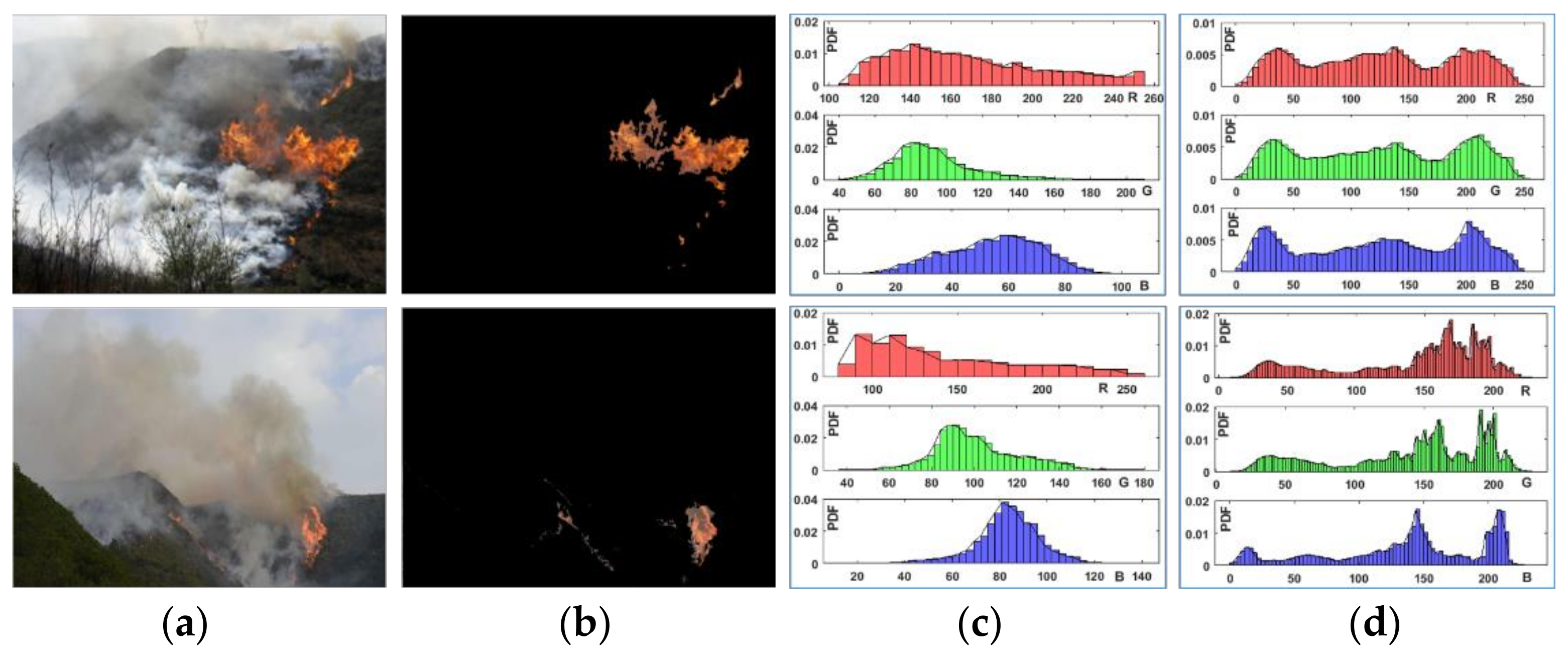
To clarify the above opinions, Figure 1 shows an example on pixel distribution. A pixel in the annotation image is filled with the original pixel if it is from the fire (positive) class; otherwise, it is filled with the values (0, 0, 0), as shown in the panel (b). Additionally, the panels (c) and (d) show the marginal distributions of the fire and non-fire pixels, respectively. Here, pixel distributions are characterized by probability density functions (PDF, for short). It shows that the distribution of positive classes tends to be unimodal; however, for the non-fire one, it tends to be a complex multi-modal distribution. Furthermore, in computation, estimating a unimodal PDF, e.g., by a Gaussian, is much easier than multi-modal PDF. Following this idea, a direct ambition is to seek a compact Gaussian “sphere”, satisfying that all fire samples are included inside, and simultaneously, as many as possible non-fire samples are excluded outside. Additionally, considering the requirements of real-time and high-precision video detection together, we aim to propose a supervised method based on the one-class model. Compared with start-of-the-art methods, the main advantages lie in three-fold: (1) This method is easier to use, either in sample collection or model training; (2) it has a solid theoretical base, e.g., following the principle of data distribution; (3) it has more potential in the real-time and high-precision detection, and does not need to consider extra feature constructions or color-space transformations.

The rest of this work is organized as below. In Section 2, the data used in this paper, including forest fire images, ground-, and UAV-monitoring videos, are presented. Our method will be detailed in Section 3, including the modeling and solution, and geometrical interpretation. To verify the performance of our proposal, experimental verification is arranged in Section 4. We conclude the whole paper in Section 5.

2. Materials and Methods

2.1. Data and Annotation

As Toulouse et al. addressed [23], infrared images or videos are easier to process than visible ones, e.g., by image thresholding, because the intensity of the fire pixels is usually higher than that of non-fire ones. In this work, we focus on the visible videos. The next three real forest fire videos will be briefly reviewed as follows.

2.1.1. Fire Video Data

The first video is dead-directional, named ForestAVI. Correspondingly, the original file “forest2.avi” can be available at http://signal.ee.bilkent.edu.tr/VisiFire/Demo/FireClips/ (accessed on 31 October 2022). This video is provided by VBI LAB, Bilkent University, Turkey. It lasts for nearly 16 s with a total of 245 frames at 15 fps (frame per second), with a fixed frame resolution at 400 × 256.

The second one is omni-directional, with the RGB-mode mp4 data format provided by Chinese CCTV video news [24]. At present, it is available at https://www.ixigua.com/6670257541009637901?logTag=0c75a9f87051eb1f91ba (accessed on 31 October 2022). This fire accident happened on 19 March 2019. The place is located at 42°25′ N and 130°38′ E, near to Jingxin Town, southeast of Hunchun city of Jilin Province, a border area between China and Russia. This video lasts 3′5″, with the speed at 25 fps and the resolution at 854 × 480. It is made up of multiple clips, including spot coverage, fighting facilities preparation, personnel schedules, and multiple fire video clips. For the convenience of fire video detection, those unrelated clips and texts, e.g., news subtitles or TV station logos, are cropped. Then, the obtained video is named CCTVmp4 in this paper, with a frame size of 854 × 288.

Different from the above two ground-monitoring videos, the third one is from aerial imagery FLAME (Fire Luminosity Airborne-based Machine Learning Evaluation), using drones located at the ponderosa pine forest on Observatory Mesa, in Northern Arizona, USA. This aerial pile burn detection database consists of different repositories. Among them, the first raw video recorded using the Zenmuse X4S camera will be used in this paper. The format of this file is also MP4. The duration of the video is 966 s with a fps of 29. The size of this repository is 1.2 GB. It is available at: https://ieee-dataport.org/open-access/flame-dataset-aerial-imagery-pile-eburn-detection-using-drones-uavs (accessed on 31 October 2022) [25]. The prescribed fire took place on 16 January 2020, with a temperature of 6 °C, partly cloudy conditions, and no wind.

2.1.2. Fire Annotation

Other materials, e.g., fire images and annotations, can be available at https://goo.gl/uW7LxW (accessed on 31 October 2022) and the references [23,24,26], for the convenience of readers. If needed, the related images, videos, and MATLAB codes for fire annotation used in this paper are also available at https://github.com/xbyang1000/fire-pixel-annotation/ (accessed on 31 October 2022).

2.2. Method

In view of the two-class classification, an image is usually defined as below,

$$P(z)=P({\omega }_1)\cdot p_1(z|{\omega }_1)+(1-P({\omega }_1))\cdot p_2(z|{\omega }_2)$$

(1)

where $z$ denotes a random pixel. The prior probability, $P({\omega }_1)$, is a pre-specified constant, e.g., estimated by fire risk index (FRI) [27]. Both PDFs, $p_1(\cdot )$ and $p_2(\cdot )$, are used to characterize the so-called unimodal or multi-modal distributions. In computer vision and pattern recognition, they both are usually estimated by a Gaussian and GMM (Gaussian Mixed Model) [12], respectively.

For our concerned one-class model, the core is to seek an ideal closed “ball”, such that: (1) all fire samples should be contained inside; (2) the ball should be so compact that as many non-fire samples as possible are excluded outside. Due to without considering non-fire supervisions, the model training just depends on the one-class fire samples. Therefore, the selected fire samples should match the distribution of the fire pixels.

2.2.1. Modeling

Suppose that $n$ fire samples are collected from the studying scene, denoted by $X=\{x_1,\cdots ,x_n\}$. To improve the computational power of learning machines, the leading optimization problems are usually discussed in a kernel-induced feature space with implicit mapping, defined as $\varphi :X\to F$. Correspondingly, the images of the low-dimensional inputs are denoted by $\varphi (X)=\{\varphi (x_1),\cdots ,\varphi (x_n)\}$, for $\forall \varphi (x_i)\in F$. Inspired by the support vector data description (SVDD) [28,29], the one-class model for the ball can be defined as the following optimization:

$$\begin{array}{c}\underset{R,a}{\min }{R}^2+C\cdot 1\prime \xi \\ s.t. \left|\right|\varphi (x_i)-a|{|}^2\le R^2-{\xi }_i\\ {\xi }_i\ge 0,i=1~n\end{array}$$

(2)

where $a$ and $R$ denote the center and radius of the desired ball, respectively. $\xi =({\xi }_1,\cdots ,{\xi }_n)\prime$ denotes a non-negative slack vector. The bold symbol $1$ denotes a constant vector. The parameter $C$ is a trade-off between the empirical error and the model generalization.

Equation (2) states that the obtained minimal ball can enclose all fire samples inside because of i.i.d. Conversely, the samples out of the ball will be classified to the non-fire class. Here, the needed compactness is characterized by minimizing $R$ and $\xi$. That is, if setting $\xi =0$, this ball will be the most compact one. However, this is not always the case, because, for a real forest scene, there may be noise samples, or called “outliers”, in the collected data. To resist potential outliers, we also introduce the slack into Equation (2). Additionally, for easy computation, here, the distances of feature samples to the center are squared, so does the radius $R$.

2.2.2. Solution

Construct a Lagrange function on (2) and let its deviations be zero w.r.t. $R$, $a$, and $\xi$, such that the problem (2) is led to the dual quadratic programming (QP), as described in matrix form:

$$\begin{array}{l}\underset{\alpha }{\min }\alpha \prime K\alpha -diag(K)\prime \alpha \\ s.t. 0\le \alpha \le C\cdot 1, 1\prime \alpha =1\end{array}$$

(3)

where $K$ is the kernel matrix with $K_{ij}=k(x_i,x_j)$, for $\forall x_i\in X$. The operator $diag(\cdot )$ means matrix diagonalization. Here, $\alpha$ is the Lagrange multiplier.

Equation (3) is a standard convex QP problem, and it is easy to solve. In practice, there have been many tools for this QP solution. For example, problem (2) can be directly solved by LIBSVM, a toolbox coded in C++ language (https://www.csie.ntu.edu.tw/~cjlin/libsvmtools/#libsvm_for_svdd_and_finding_the_smallest_sphere_containing_all_data, accessed on 31 October 2022). Additionally, due to the equivalence between the dual problems of SVDD and one-class SVM, the solution of (3) can also be obtained by the MATLAB toolbox named “Statistics and Machine Learning Toolbox”. Note that here, one-class SVM can also be viewed as a two-class classification method, i.e., by separating the coordinate origin (negative) from the given one-class data (positive).

Considering the real-time requirement, next, we come to the batch decision for the pixel-precision video detection.

2.2.3. Decision Making in Batch

It is easy to know that, for a candidate pixel-pattern sample, $z$, the decision function can be defined as $f(z)=\mathrm{sgn}(R^2-||\varphi (z)-a|{|}^2)$. Correspondingly, the decision rule for $z$ is that, if $f(z)\ge 0$, $z\in {\omega }_1$, i.e., it is assigned to the fire class; otherwise, $z\in {\omega }_2$. It is obvious that such a pixel-by-pixel decision is inefficient. In a real-time video detection, the decision making should be carried out at least in batch, e.g., the pixels in the same frame can be determined by the one-time calculation. Suppose there are $m$ pixel-pattern samples, denoted by $X^{(t)}=\{x_1^{(t)},\cdots ,x_m^{(t)}\}$, here, $m$ is the number of frame pixels. For easy reading, the batch decision is described in Theorem 1.

Theorem 1. 

Given a test sample matrix $X^{(t)}$, a ball  $B(a,R|\alpha )$ w.r.t., and the training set  $X$, the batch decision for  $X^{(t)}$ can be made by the signs of the vector  $(T\cdot 1-K^{(t)}\alpha )$, where  $T$ is a constant, and  $K^{(t)}$ is an  $m\times n$ kernel matrix.

The proof is provided in Appendix A. From (A2), the computation load of the batch decision mainly focuses on computing $K^{(t)}$, which is determined by the sparsity of $\alpha$. Setting $0<\alpha <1/(\tau n),\tau \in [0,1]$, thus, $\tau$ can be used to balance the computation and compactness, e.g., by selecting appropriate support vectors. This will be interpreted in the next subsection.

2.2.4. Interpretation

Figure 2 shows an example for our desired one-class model, in which the fire pixels are drawn from the first image of Figure 1, as shown as blue dots in the 2D or 3D figures. For easy visualization, the obtained 3D ball, corresponding to the decision domain of the fire pixels, is shown from three different viewpoints, i.e., by using R-G, R-B and G-B color spaces. Visually, the decision plane is shown as a magenta contour with the value 0. Another two auxiliary planes, named the support plane with the value 1 or −1, are used to illustrate the compactness of the ball, as shown in the red or green contours, respectively. The result is that the obtained decision plane is clearly biased to the interior contour, though it is equidistant to both support planes. This means that the obtained ball is compact. Additionally, it also shows that some dots are out of the ball because they are detected as outliers. In doing so, the obtained decision plane can be smoother, which is very important for the model’s generalization.

Figure 3 is to explain the trade-off between real-time computation and the compactness of the one-class model. For the decision boundary in Figure 2b, three groups of support vectors are shown in Figure 3a–c, subject to the different scale parameter $\tau$ at 0.7, 0.3, and 0.1, respectively. This trade-off can be visualized and explained by the number and locations of these support vectors. For example, in Figure 3a, there is only a total of 17 support vectors needed to be stored after model training, while less support vectors mean better real-time detection because of the lower-order matrix computation. If increasing the number of support vectors, as shown in Figure 3b,c, more interior samples will be viewed as support vectors. With the increase in the number of support vectors, the performance of real-time detection would be worse. Therefore, for a real application, this parameter should be tuned carefully, which will be detailed in the experiment section.

3. Results

3.1. Experiment Setup

As described in Section 2.1, the fire videos used for the verification are briefly introduced in

Table 1. Video brief information.

Video Name	Resolution	Duration	Total Frames	Frame Rate	Video Mode
ForestAVI	400 × 256	16″	245	15 fps	Static, ground 1
CCTVmp4	854 × 288	15″	376	25 fps	Dynamic, ground
FLAME	1280 × 720	966″	28,080	29 fps	Dynamic, UAV

¹. The “static, ground” mode means that it is a static-background video obtained by a ground-monitoring camera. Likewise, the mode “dynamic, UAV” is a dynamic-background UAV-based video.

, including video resolution (width × height) and duration (in seconds), total of video frames (total frames), frame rate (in frame per second, fps), and the video-monitoring mode.

Throughout the whole paper, the truth for a pixel is provided by the pixel-level annotation method, for more details, please see [23,24]. In contrast to the state-of-the-art methods, we take three popular fire detectors as baselines, i.e., YCbCr rule-reasoning (rule, for short) [4,30], unsupervised k-Medoids (Medoids) [14,15], and supervised SVM-based (SVM) [12,13] methods. The ground truth (GT) used in this section is provided by the interactive fire pixel annotation [24].

For the convenience of visualization and computation, video processing and method implement are executed on MATLAB platform, or associated with the toolbox “Statistics and Machine Learning”. The pixels of the first frame of each video are used for model training, and the rest frames are for the testing. Under the guidance of GT, the training set is composed of two-class pixel-pattern samples, randomly drawn from the first frame. To avoid unbalance classification, the number of training samples is determined by the minority of two-class pixels. For the unsupervised k-Medoids method, the fire cluster is determined by the closest inter-cluster-center distance to the fire (positive) training samples. For the proposed one-class model, the solution is obtained by one-class SVM with the RBF kernel function. Both the SVM and one-class SVM are solved by the MATLAB function “fitcsvm”, but with different parameter settings. In detail, the regularization parameter C in SVM is adaptive, which is tuned by the parameter “BoxConstraint” in “fitcsvm” with the default value 1. For the fairness of using supervisions, one-class SVM is just trained on the positive samples, also with the RBF kernel. Instead of C, the regularization parameter $\tau$ in the one-class model is tuned in the range [0, 1] for the compactness, by tuning “nv” in “fitcsvm”. The YCbCr rule-based method is executed on YCbCr pixels. Therefore, it needs a space transformation, generally, from RBG to YCbCr, because the RGB color model is the most popular mode in video data acquisition, e.g., a RGB24 data format with three 8-bit channels. We also provide a demo for the fire video detection by using one-class SVM. If needed, it can be available at https://github.com/xbyang1000/OneClassDemo (accessed on 31 October 2022)

All comparisons are conducted on a Dell PC (Landrock, TX, USA), with Intel Core 2 Quad CPU @2.83 GHz (Santa Clara, CA, USA) and 4G RAM (Seoul, Seoul, South Korea), running MATLAB 2017b (Natick, MA, USA) in a windows 7 operating system (Redmond, WA, USA).

3.2. Experimental Results

3.2.1. Evaluation Indicators

This work is oriented to fine-grained video detection, which is different from the coarse-grained video detection, e.g., block-based (video frame or the frame-partitioned rectangle blocks) detection with deep learning methods. Towards the goal of pixel-precision and real-time detection, four indicators will be used to evaluate the performance of our proposed method extensively, including fire detection rate (TP: True Positive), error warning rate (FP: False Positive), fire positioning (Pixel Location) and detection time (Time) in seconds. For a given pixel, here, TP means that if the truth is positive (annotated as a fire pixel), the test predicts positive; otherwise, it is called FP. The indicator for fire positioning means that if it is recognized as a fire pixel, the position (location) of the pixel in the frame should be returned. The detection time refers to the total time of detecting all pixels in a frame. If it is less than the acquisition time, e.g., 0.345 s (1/29) in the FLAME video, the detection can be viewed as real-time.

Next, the fire-detected results are divided into two parts. The first part shows the result of the several selected video frames in visualization; in the second part, the detected results are detailed on each video frame.

3.2.2. Comparison on the Selected Video Frames

To show the result easily, in this subsection, the test set is composed of four time-discontinuous frames, drawn from the (f/i)-th frame, i = 4~1, respectively, where f is the total of video frames. In Figure 4, the fire detection results are shown in the rightmost four columns, with the original pixels of the test frame if they are identified as fire pixels, or with the black pixels otherwise. Since the model is trained on the studying scene, both SVM and one-class SVM are able to achieve higher fire detection rates and lower error warning rates at the same time. It is worth mentioning that they both also have an ability in error correction, compared with the ground truth of the last test frame in the data “CCTVmp4”, in which the red firefighters’ clothing is error-annotated as fire pixels. Additionally, a fire flame area detected by our one-class model seems slightly smaller than that of GT or SVM, as shown in Figure 4. In contrast, the rule-reasoning and k-Medoids methods are also capable of capturing fire; however, they usually suffer from over-high error warning rates, as shown those non-fire pixels appeared in the detected figures.

3.2.3. Comparison on Every Video Frame

In order to show the performance of the proposed method extensively, in this subsection, we aim to report the comparison on every video frame. This is also measured by using the above-mentioned quantified indicators. Especially for the indicator fire positioning, the “fire location” is usually quantified as a ratio of the area of the detected fire flame to that of the test frame. Thus, this result on each frame can be shown in the same figure, as suggested in the reference [30]. Here, due to the equal frame-size in the same video, the area of the fire flame can be approximated by the number of fire pixels. For example, in the case that there are 100 fire pixels in the current frame with a fixed frame size of m × n, and a fire detector, e.g., SVM, can identify all pixels correctly, i.e., absolutely achieving the fire detection rate at 100% and the error warning rate at 0%, the value of the fire area ratio should be 100/(mn), where the numerator and denominator denote the number of fire pixels and a total of frame pixels, respectively. If the predicted ratio approaches or even equals to that of GT, we can say that the detected fire pixels have been positioned accurately. That is, the proximity of the area ratios between the predicted result and GT can be used to measure the accuracy of fire positioning.

In Figure 5, four indicators are used to evaluate the performance, as shown in the corresponding panels. From the left to the right, they are the fire detection rates (in percentage), error warning rates (in percentage), fire flame area (in percentage), and detection time (in seconds), as shown in vertical axes, respectively. To show the details easily for the error warning rates and detection time, these vertical coordinates are shown in the logarithm, but with original values on the axes. Here, the logarithm means the natural logarithm ln(.). Since the first frame has been used for the model training, the rest of the frames indexed by 2 to f are used for testing, as shown in the horizontal axes, where f denotes the total number of the video frames. For each indicator (panel), four colored lines present the different detected results obtained by four fire detection methods, respectively. Additionally, the cyan “reference lines” are introduced to show the ground truth or ideal value. For example, the cyan line in Panel (a) shows an ideal value at 100% for the fire detection rate, while in Panel (c), the ground truth of the fire flame area is used for measuring the fire positioning. That is, if a predicted value is close to this reference value, it means that in the current frame, accurate fire positioning for all fire pixels has been achieved. Note that on the data FLAME, due to the high-resolution and huge number of frames, the results of k-Medoids clustering are unavailable because this method is very time-consuming and meaningless for real-time detection.

4. Discussion

The first three indicators, i.e., fire detection rate, error warning rate, and fire positioning, are visualized in Figure 4. The results show that among the four fire detection methods, the supervised SVM and one-class SVM are superior, then the YCbCr rule-based method follows. The slight difference between the SVM and one-class SVM regards the area of the detected fire flames. This may be explained by the compactness, due to the fact that: (1) The fire pixel distribution cannot be well represented by the selected fire pixels. According to the interactive image annotation method [24], the fire samples used for training a KNN classifier are selected from the pixels that are most likely to be flames, e.g., usually selected from the central region of the fire flame; (2) Because of the compactness, the area of the fire flame tends to be smaller than that of SVM. Different from the baselines, here, the one-class method is originated from the i.i.d. hypothesis. Therefore, in view of machine learning, it will be better if the fire samples for training a one-class model are selected from a complete flame region.

Extensive results on all video frames are shown in Figure 5. Among the four indicators, both fire detection rates and error warning rates can be used to measure the performance of fire detection. In this view, an ideal detector should be able to achieve a high-fire detection rate and a low-error warning rate at the same time. Towards this goal, both SVM and our one-class model outperform the other two. Concretely, as for the fire detection rate, the YCbCr rule achieves the highest fire detection rate on the first two videos; however, on the third one, it seems unstable and the obtained fire detection rates vary from 40% to 100%. In contrast to the results of the first two data, due to the long-distance in UAV-monitoring, the flame areas of the third video are always small, as shown by the cyan reference line (GT) in Figure 5c and the test fames in the last row of Figure 4. That is, a small number of miss-detected fire pixels may result in a big oscillation in the fire detection rate. This explanation can also be used for the k-Medoids. If together with the error warning rate, in general, over-high error warning rates make both unsupervised methods unsuitable for forest fire detection, especially in the complex forest scenes. Furthermore, if further considering the requirement of real-time, the situation will be even worse. The predicted values of the detection time are always greater than the reference values. Visually, as shown in Figure 5d, the line of the predicted values is always above the cyan reference line. Here, the reference value is measured by FPS (frame per second), with the real-time value of 1/fps second. In the detection time, both supervised methods are superior and able to satisfy the requirement of real-time detection on the first two videos. However, due to a high resolution, they cannot satisfy the requirement on the third video, i.e., the real-time value of 0.0345 s per frame (1/29). Moreover, it is also a big challenge for the current computation and vision-based recognition techniques. In order to suit this requirement, the frame-skipping detection should be the second best, as shown in the right-bottom figure, where another cyan wider reference line means a 10× delay, i.e., the value of 0.345 s.

At the end, let us come to fire positioning. In a real forest fire monitoring, the ability of an accurate fire location can help us in two aspects: (1) it can be used to measure the performance of a fire detector, and (2) it is useful for a fire emergency rescue, especially in the stage of early fire. If returning the pixel coordinates, it is a direct and intuitive representation for fire positioning, e.g., in the manner of visualization. However, it is unsuitable for video detection if want to show the result in a frame-by-frame manner. To relieve this dilemma, the pixel coordinates in the same frame can be replaced with the area of the detected fire flame. Visually, if the predicted value is close to the area of GT, the accurate pixel positioning of the whole frame can be achieved. In other words, the accuracy of the fire positioning can be measured by the consistence between the predicted line (or values) and the GT line. Here, the consistency includes the proximity and change trend. As shown in Figure 5c, tendencies of three lines, i.e., the predicted values of SVM, our one-class model, and GT, respectively, are consistent. This means that both SVM and our one-class model are capable of accurate fire pixel positioning. Therefore, if considering the above indicators together, the one-class model is the best method for the forest fire video detection.

5. Conclusions

In this work, we propose a new method for forest fire video detection. It is oriented on pixel distribution, i.e., the i.i.d. hypothesis, which is significantly different from the existing methods. Inspired by the supervised fire detectors and the empirical results of the unimodal fire pixel distribution, we develop a one-class model for fire detection. In computation, the leading problem can be solved by a convex QP optimization. To speed fire detection, we also provide a strategy for batch decision-making. Due to the compactness of the one-class ball, it can be used for controlling the error warning rate. Compared with the state-of-the-art methods, the comparison on the forest fire videos shows its superiority in a higher fire detection rate, a lower error warning rate, more accurate fire location in positioning, and the fastest detection speed. In computation, although it can be solved by one-class SVM, a variant of SVM, it differs from SVM in three-fold: (1) It needs less supervision information for model training. For example, in a balance classification, training a one-class model just depends on the positive samples, nearly half of the training set for SVM; (2) It is easy to use without considering non-fire information. In fact, it is not easy for training a two-class or multi-class model on how to select negative samples; (3) Due to the unimodal distribution, the obtained decision domain is bounded, i.e., the “ball” in geometry for the fire pixels. However, for SVM, it aims to separate the input space into two disjointed half-spaces. Therefore, its decision domain may be unbounded or not. Even if it is bounded, it is still unclear whether it is formed by the joint action of both classes of samples or by the single action of one class. This can be used to explain that if selecting training samples carefully, sometimes a better detection result can also be obtained without considering the data distribution for a two-class or multi-class method. In this case, if the obtained decision boundary is tight enough for one of the multi-class training samples, e.g., the fire class, in essence, the data distribution is applied subconsciously in the sample selection.

Different from the general object recognition, the difficulties for fire recognition are that: (1) As a special object, fire is non-rigid, shapeless, has color uncertainty, and is made up of many complex substances. Until now, it is still unclear what features are conducive for extracting a fire flame; (2) Due to the complexity of various forest scenes, public fire images and video databases with high-precision annotations are still few or unavailable [31]; (3) In a practical view, a forest fire detector should be evaluated by multiple indicators, e.g., the fire detection rate, error warning rate, real-time, and fire location (for the fire-spread trend prediction and fire rescue), rather than a single indicator such as test accuracy in the general object recognition; (4) It frequently suffers from an unbalance classification problem, especially at the early fire stage.

Furthermore, in view of the independently and identically distributed (i.i.d.) hypothesis in machine learning, it is a little far-fetched for viewing fire detection as a binary classification. For example, it is unreasonable for those non-fire objects, composed of sky, ground, trees, plants, etc., to be viewed from the same class. However, if viewing it as a multi-class classification to reduce the dependence on the i.i.d. hypothesis, what should be the appropriate number of classes (categories) for a scene-changing forest environment? Additionally, for a large-scale dataset, SVM tends to be extremely cumbersome, e.g., is intolerant time- or memory-consuming. In the literature, many variants or called approximators have been proposed, such as LSSVM (least square SVM), TWSVM (TWin SVM) [32], PSVM (Proximate SVM), and newly FSVC (fast SVM) [31]. If using them for fire detection, the performance also remains to be studied. In this paper, our method is oriented from pixel classification, and fire detection is expected to be accomplished in one-time scanning. Due to the high-precision real-time detection and model interpretability, there is no comparison with deep learning-based methods. Additionally, for a given forest scene, if fire information is insufficient or unobtainable, how to train a machine to match this fire-absent scene? Obviously, it is a bigger challenge in forest fire detection. Our potential avenue for future research also involves smoke detection and its relation to fire.

References

1. Bao, S.; Xiao, N.; Lai, Z.; Zhang, H.; Kim, C. Optimizing watchtower locations for forest fire monitoring using location models. Fire Saf. J. 2015, 71, 100–109. [Google Scholar] [CrossRef]
2. Chinese State Statistical Bureau. Statistical Yearbook of China in 2018. Available online: http://yearbookchina.com/navipage-n3018103001000742.html (accessed on 7 May 2019). (In Chinese).
3. Ying, L.; Han, J.; Du, Y.; Shen, Z. Forest fire characteristics in China: Spatial patterns and determinants with thresholds. For. Ecol. Manag. 2018, 424, 345–354. [Google Scholar] [CrossRef]
4. Çelik, T.; Demirel, H. Fire detection in video sequences using a generic color model. Fire Saf. J. 2009, 44, 147–158. [Google Scholar] [CrossRef]
5. Chen, T.-H.; Wu, P.-H.; Chiou, Y.-C. An Early Fire-Detection Method Based on Image Processing. In Proceedings of the 2004 International Conference on Image Processing, Singapore, 24–27 October 2004; Volume 3, pp. 1707–1710. [Google Scholar]
6. Bu, F.; Gharajeh, M. Intelligent and vision-based fire detection systems: A survey. Image Vis. Comput. 2019, 91, 103803. [Google Scholar] [CrossRef]
7. Foggia, P.; Saggese, A.; Vento, M. Real-time fire detection for video surveillance applications using a combination of experts based on color, shape and motion. IEEE Trans. Circuits Syst. Video Technol. 2015, 25, 1545–1556. [Google Scholar] [CrossRef]
8. Qureshi, W.S.; Ekpanyapong, M.; Dailey, M.N.; Rinsurongkawong, S.; Malenichev, A.; Krasotkina, O. Quickblaze: Early fire detection using a combined video processing approach. Fire Technol. 2016, 52, 1293–1317. [Google Scholar] [CrossRef]
9. Gaur, A.; Singh, A.; Kumar, A.; Kumar, A.; Kapoor, K. Video Flame and Smoke Based Fire Detection Algorithms: A Literature Review. Fire Technol. 2020, 56, 1943–1980. [Google Scholar] [CrossRef]
10. Maeda, E.E.; Formaggio, A.R.; Shimabukuro, Y.E.; Arcoverde, G.F.B.; Hansen, M.C. Predicting forest fire in the Brazilian Amazon using MODIS imagery and artificial neural networks. Int. J. Appl. Earth Obs. Geoinf. 2009, 11, 265–272. [Google Scholar] [CrossRef]
11. Bui, D.T.; Hoang, N.-D.; Samui, P. Spatial pattern analysis and prediction of forest fire using new machine learning approach of Multivariate Adaptive Regression Splines and Differential Flower Pollination optimization: A case study at Lao Cai province (Vietnam). J. Environ. Manag. 2019, 237, 476–487. [Google Scholar]
12. Ko, B.C.; Cheong, K.-H.; Nam, J.-Y. Fire detection based on vision sensor and support vector machines. Fire Saf. J. 2009, 44, 322–329. [Google Scholar] [CrossRef]
13. Duong, H.; Tinh, D.T. An Efficient Method for Vision-Based Fire Detection Using SVM Classification. In Proceedings of the International Conference on Soft Computing and Pattern Recognition 2013, Hanoi, Vietnam, 15–18 December 2013. [Google Scholar]
14. Khatami, A.; Mirghasemi, S.; Khosravi, A.; Lim, C.P.; Nahavandi, S. A new PSO-based approach to fire flame detection using K-Medoids clustering. Expert Syst. Appl. 2017, 68, 69–80. [Google Scholar] [CrossRef]
15. Hashemzadeh, M.; Zademehdi, A. Fire detection for video surveillance applications using ICA K-medoids-based color model and efficient spatio-temporal visual features. Expert Syst. Appl. 2019, 130, 60–78. [Google Scholar] [CrossRef]
16. Muhammad, K.; Ahmad, J.; Lv, Z.; Bellavista, P.; Yang, P.; Baik, S.W. Efficient deep CNN-based Fire detection and localization in video surveillance applications. IEEE Trans. Syst. Man Cybern. Syst. 2019, 49, 1419–1434. [Google Scholar] [CrossRef]
17. Xu, R.; Lin, H.; Lu, K.; Cao, L.; Liu, Y. A forest fire detection system based on ensemble learning. Forests 2021, 12, 217. [Google Scholar] [CrossRef]
18. Muhammad, K.; Ahmad, J.; Baik, S.W. Early fire detection using convolutional neural networks during surveillance for effective disaster management. Neurocomputing 2018, 288, 30–42. [Google Scholar] [CrossRef]
19. Wu, Z.; Xue, R.; Li, H. Real-Time Video Fire Detection via Modified YOLOv5 Network Model. Fire Technol. 2022, 58, 2377–2403. [Google Scholar] [CrossRef]
20. Dong, Y.; Zhang, F.; Joe, I.; Lin, H.; Jiao, W.; Zhang, Y. Learning for multiple-relay selection in a vehicular Delay Tolerant Network. IEEE Access 2020, 8, 175602–175611. [Google Scholar] [CrossRef]
21. Zhang, L.; Wang, M.; Fu, Y.; Ding, Y. A Forest Fire Recognition Method Using UAV Images Based on Transfer Learning. Forests 2022, 13, 975. [Google Scholar] [CrossRef]
22. Du, S.; Zhang, Y.; Sun, Q.; Gong, W.; Geng, J.; Zhang, K. Experimental study on color change and compression strength of concrete tunnel lining in a fire. Tunn. Undergr. Space Technol. 2018, 71, 106–114. [Google Scholar] [CrossRef]
23. Toulouse, T.; Rossi, L.; Campana, A.; Celik, T.; Akhloufi, M.A. Computer vision for wildfire research: An evolving image dataset for processing and analysis. Fire Saf. J. 2017, 92, 188–194. [Google Scholar] [CrossRef] [Green Version]
24. Yang, X.; Chen, R.; Zhang, F.; Zhang, L.; Fan, X.; Ye, Q.; Fu, L. Pixel-level automatic annotation for forest fire image. Eng. Appl. Artif. Intell. 2021, 104, 104353. [Google Scholar] [CrossRef]
25. Shamsoshoara, A.; Afghah, F.; Razi, A.; Zheng, L.; Fulé, P.Z.; Blasch, E. Aerial imagery pile burn detection using deep learning: The FLAME dataset. Comput. Netw. 2021, 193, 108001. [Google Scholar] [CrossRef]
26. Cazzolato, M.T.; Avalhais, L.P.; Chino, D.Y.; Ramos, J.S.; de Souza, J.A.; Rodrigues, J.F., Jr.; Traina, A.J. Fismo: A Compilation of Datasets from Emergency Situations for Fire and Smoke Analysis. In Brazilian Symposium on Databases-SBBD; SBC: Uberlândia, Brazil, 2017; pp. 213–223. [Google Scholar]
27. Zhang, F.; Zhao, P.; Xu, S.; Wu, Y.; Yang, X.; Zhang, Y. Integrating multiple factors to optimize watchtower deployment for wildfire detection. Sci. Total Environ. 2020, 737, 139561. [Google Scholar] [CrossRef] [PubMed]
28. Schölkopf, B.; Platt, J.C.; Shawe-Taylor, J.; Smola, A.J.; Williamson, R.C. Estimating the support of a high-dimensional distribution. Neural Comput. 2001, 13, 1443–1471. [Google Scholar] [CrossRef] [PubMed]
29. Todkar, S.S.; Baltazart, V.; Ihamouten, A.; Dérobert, X.; Guilbert, D. One-class SVM based outlier detection strategy to detect thin interlayer debondings within pavement structures using Ground Penetrating Radar data. J. Appl. Geophys. 2021, 192, 104392. [Google Scholar] [CrossRef]
30. Wang, Y.; Yu, Y.; Zhu, X.; Zhang, Z. Pattern recognition for measuring the flame stability of gas-fired combustion based on the image processing technology. Fuel 2020, 270, 117486. [Google Scholar] [CrossRef]
31. Hammouri, Z.; Fernandez-Delgado, M.; Cernadas, E.; Barro, S. Fast SVC for large-scale classification problems. IEEE Trans. Pattern Anal. Mach. Intell. 2021, 44, 6184–6195. [Google Scholar] [CrossRef]
32. Ye, Q.; Huang, P.; Zhang, Z.; Zheng, Y.; Fu, L.; Yang, W. Multiview learning with robust double-sided twin SVM. IEEE Trans. Cybern. 2021, 2021, 34546934. Available online: https://ieeexplore.ieee.org/abstract/document/9543472 (accessed on 31 October 2022).
Figure 1. Pixel distribution for forest fire images. (a,b) panels show the original images and the fire pixel annotations; (c,d) are the pixel distributions for the fire and non-fire objects, respectively.
Forests 13 01826 g001
Figure 2. An example for the proposed one-class model. Panel (a) shows the RGB fire pixels, corresponding to the first forest fire image of Figure 1; the panels from (bd) are used to show the desired ball in three 2D cases, respectively. Each 2D boundary of the ball is contoured as the legend with magenta lines.
Forests 13 01826 g002
Figure 3. Support vectors obtained by different scale parameter τ in the 2D R-G color space. There are a total of 17, 164, and 663 support vectors, marked with black circles “o”, as shown in the panels (ac), respectively.
Forests 13 01826 g003
Figure 4. Visualization for video detection. Panel (a) shows the first video frame, which is used for model training or providing supervision information for other unsupervised methods. Panels (b) and (c) are four test frames and the fire pixel annotation (GT). The rightmost four panels show the results of the detected fire, obtained by rule-reasoning (d), k-Mediods clustering (e), SVM (f), and our one-class model (g), respectively.
Forests 13 01826 g004
Figure 5. Fire detection results for all test frames, shown as the fire detection rate (a), error warning rate (b), fire flame area (c), and detection time (d), respectively.
Forests 13 01826 g005