
Use of Mobile Laser Scanning (MLS) to Monitor Vegetation Recovery on Linear Disturbances
 , , and
Abstract
:1. Introduction
- (1)
- To test the accuracy of using MLS to measure the height, DBH, and density of trees on seismic lines.
- (2)
- To determine whether the accuracy of data from MLS systems is impacted by leaf-on or leaf-off conditions.
2. Materials and Methods
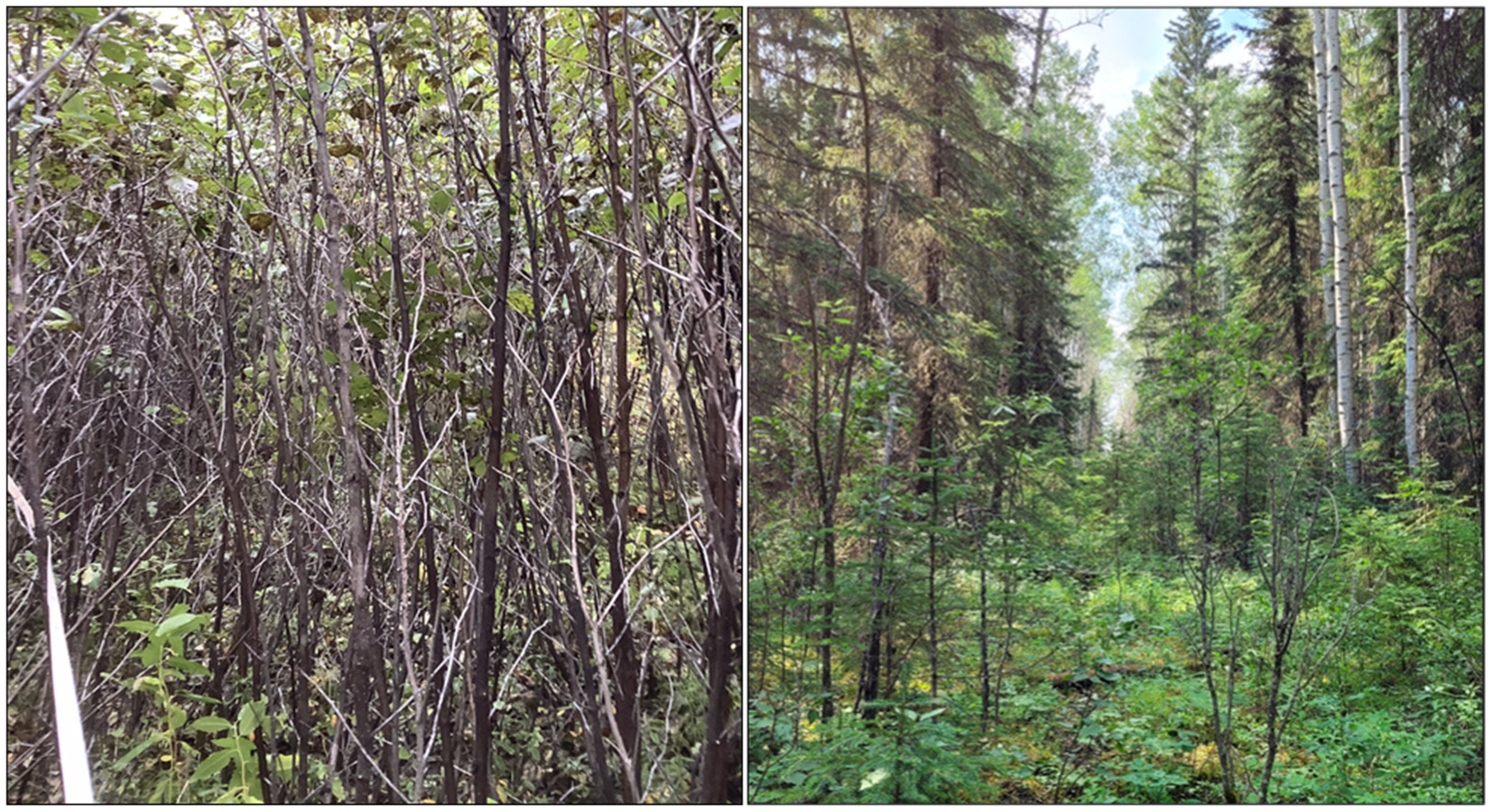
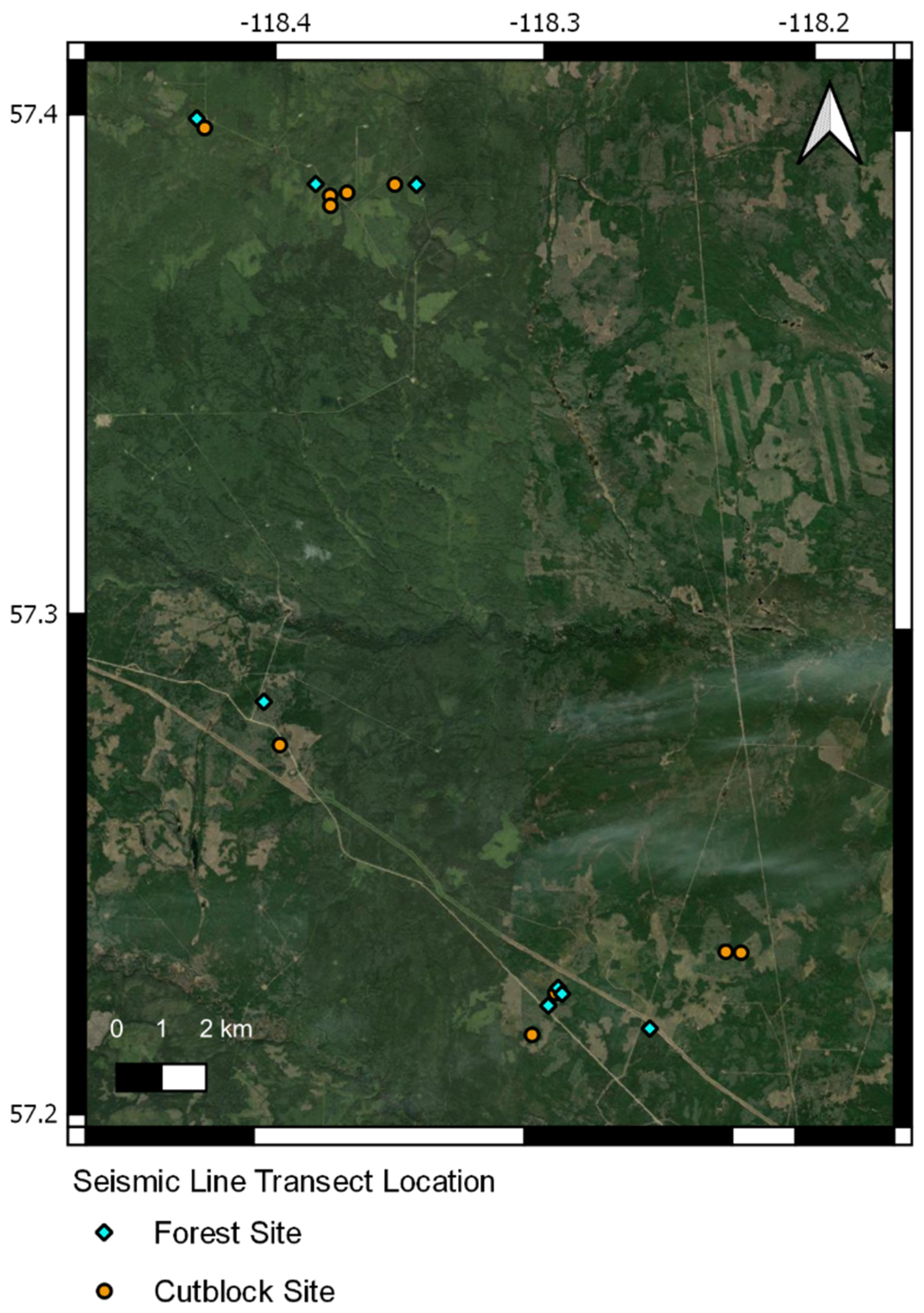
2.1. Site Selection
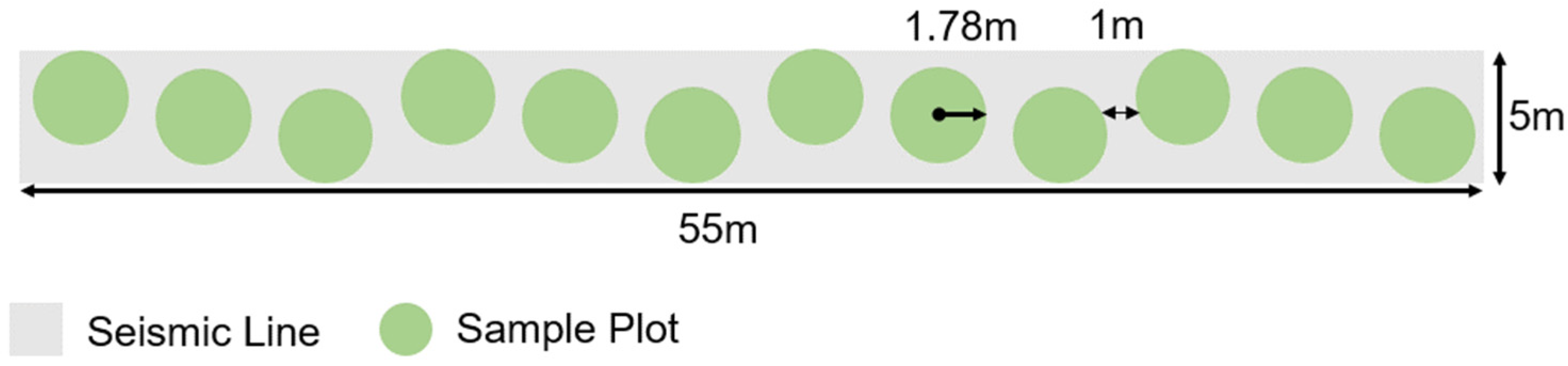
2.2. Plot Layout & Ground Reference Data Collection
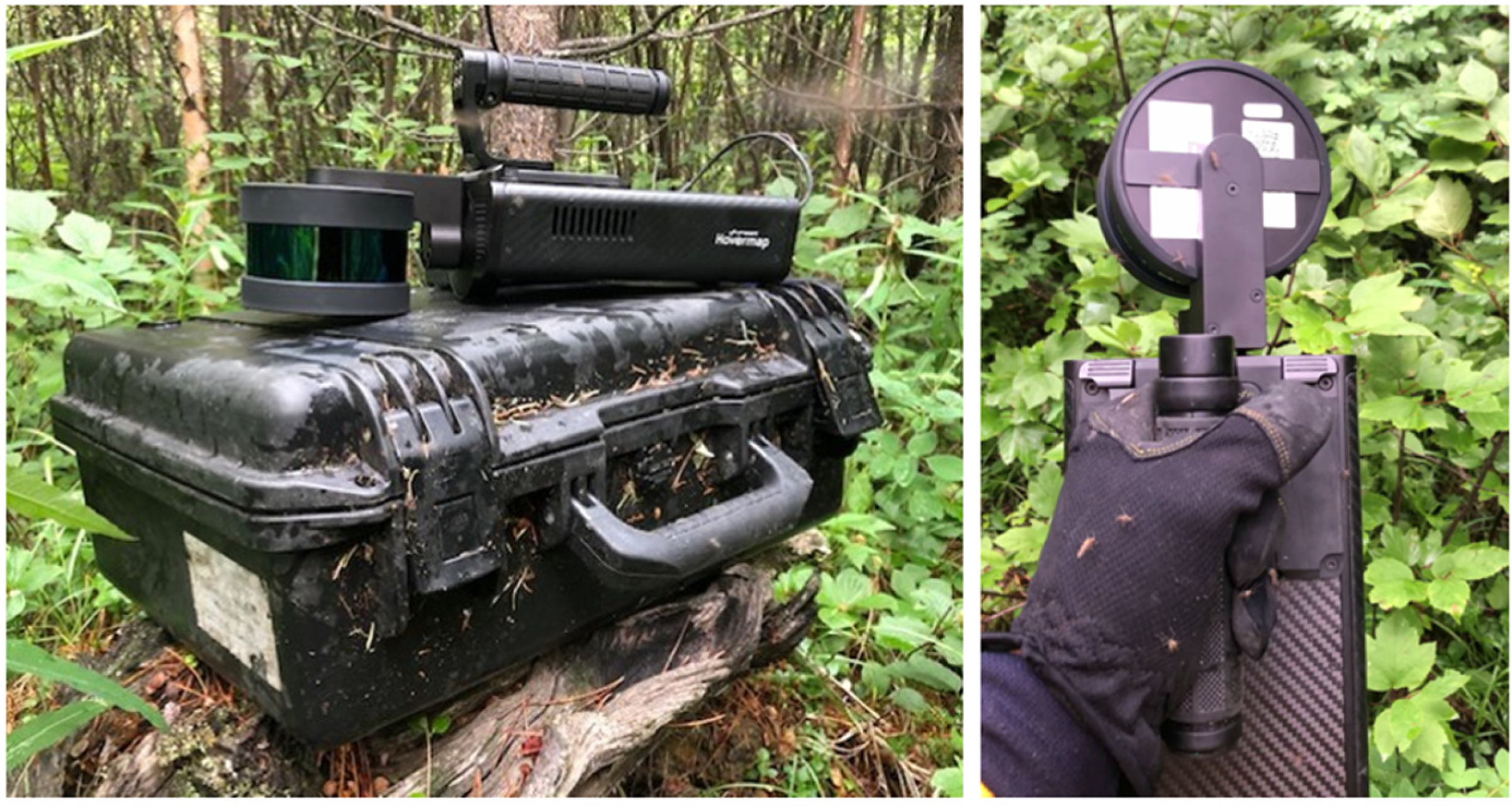
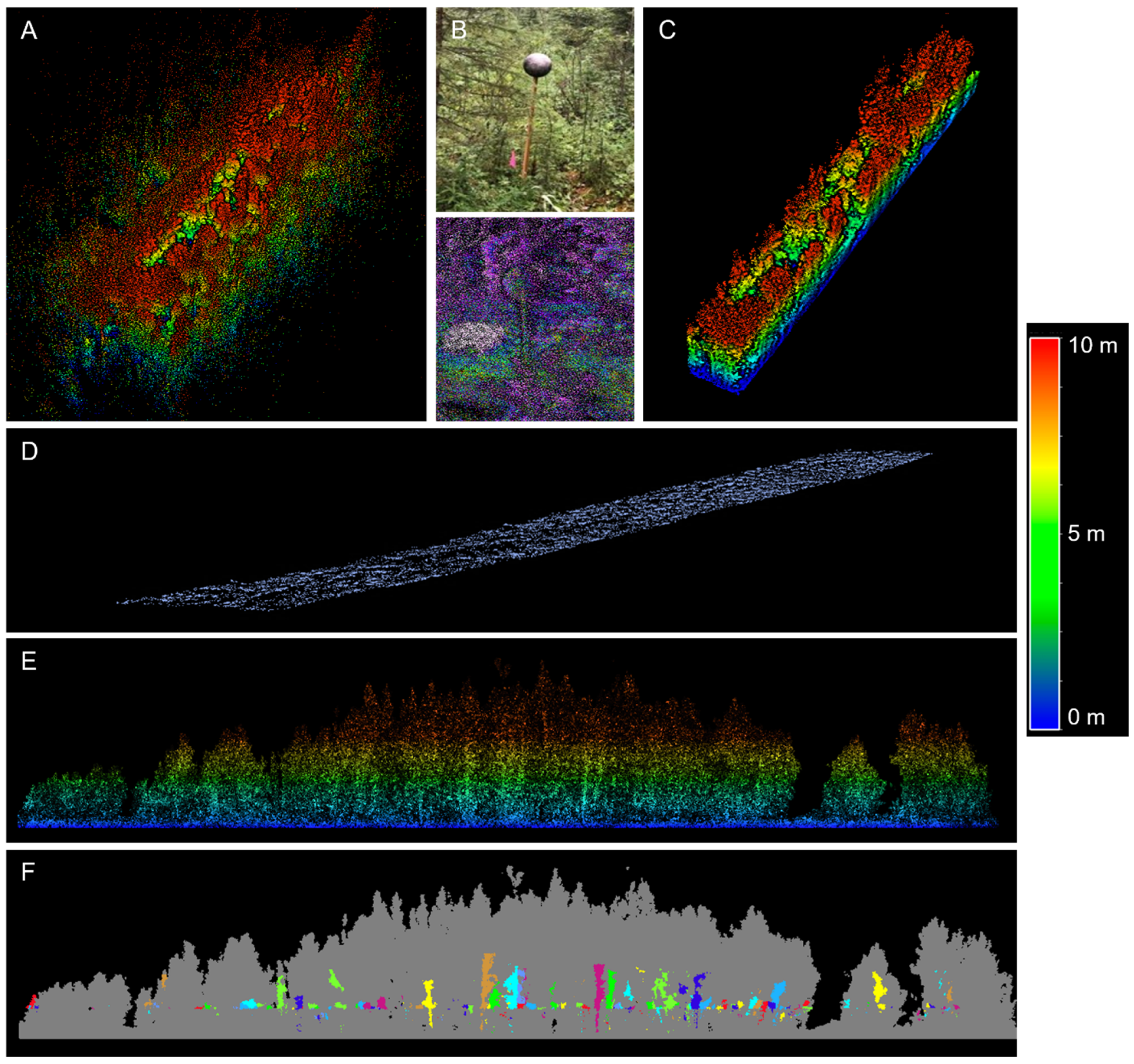
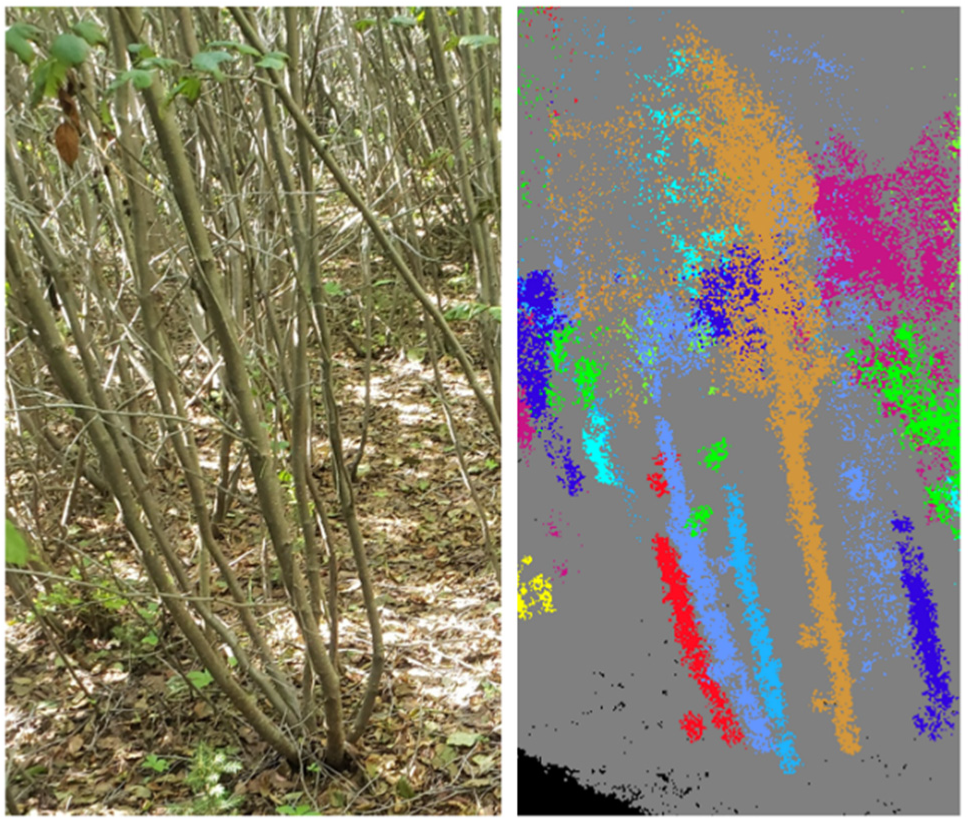
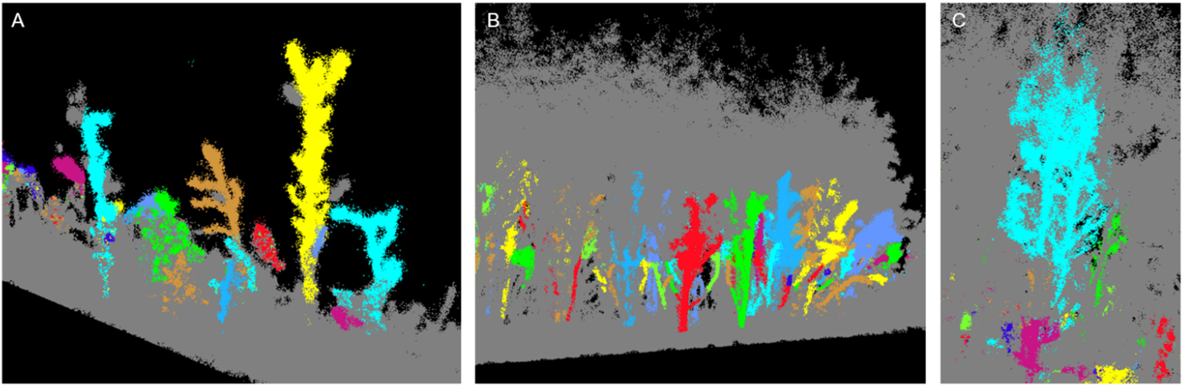
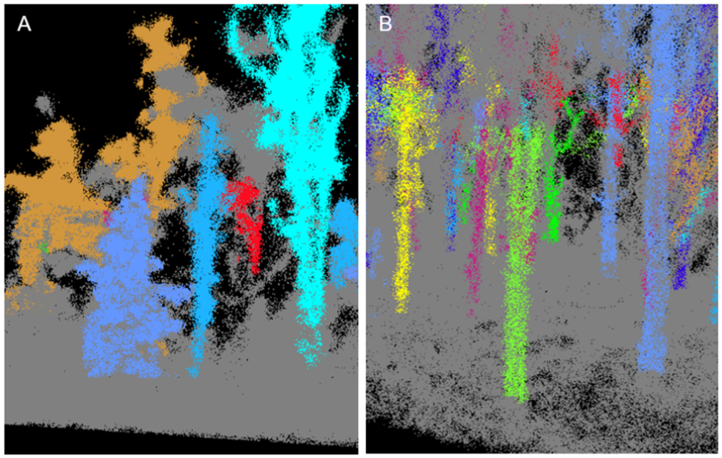
2.3. LiDAR Data Collection and Processing
2.4. Data Analysis
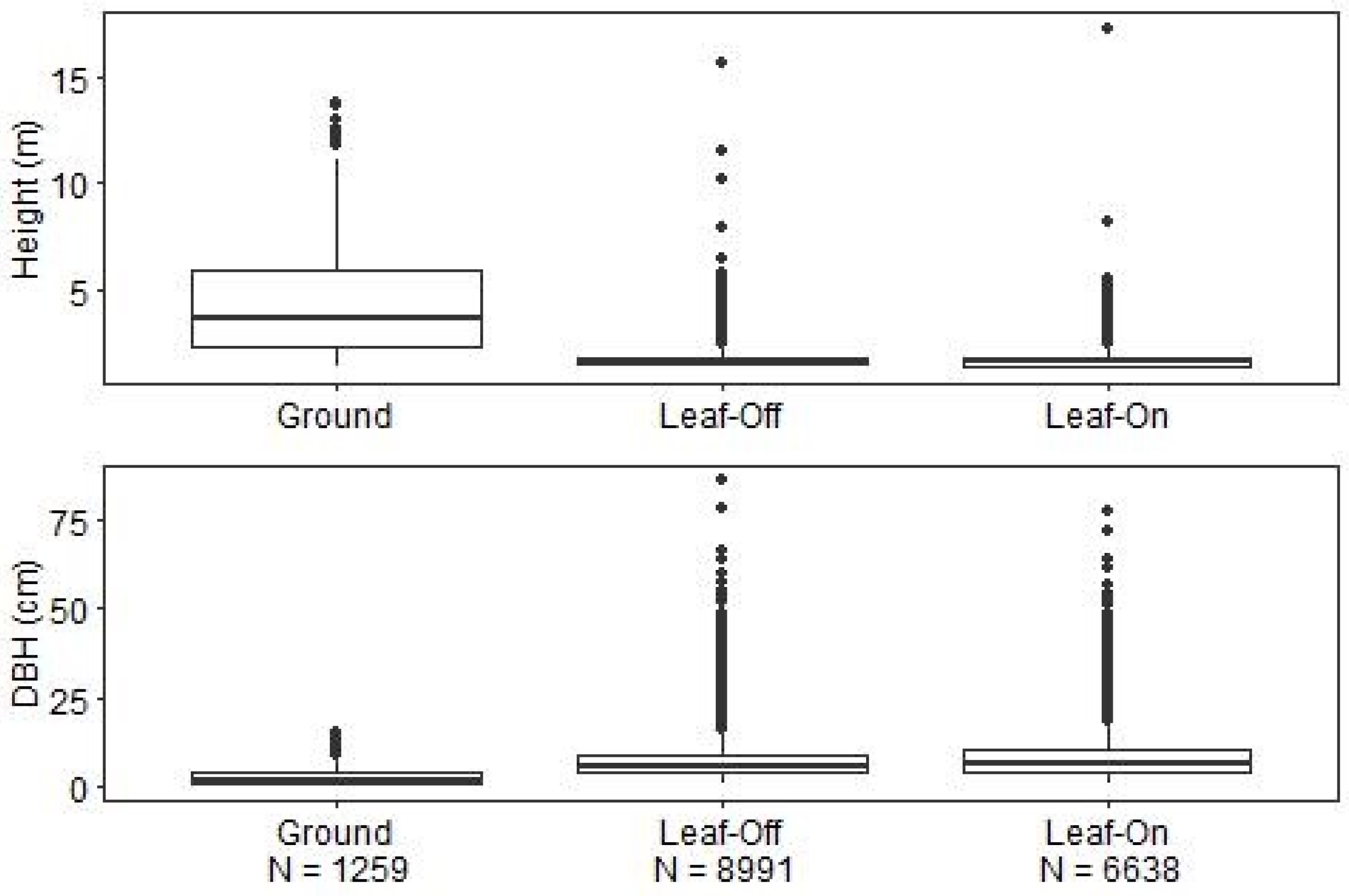
3. Results
4. Discussion
4.1. Vegetation Density
4.2. Tree Height
4.3. Tree DBH
4.4. Leaf Condition
4.5. Field Challenges
5. Conclusions
Author Contributions
Funding
Data Availability Statement
Acknowledgments
Conflicts of Interest
Appendix A

| Stand Type | Classification | Direction | Latitude | Longitude | Leaf-On Scan | Leaf-Off Scan |
|---|---|---|---|---|---|---|
| Forest | FR | NE-SW | −118.287 | 57.226 | ✔ | |
| Forest | FR | E-W | −118.429 | 57.400 | ✔ | ✔ |
| Forest | FR | E-W | −118.384 | 57.387 | ✔ | ✔ |
| Forest | FR | NE-SW | −118.254 | 57.219 | ✔ | |
| Forest | NR | NE-SW | −118.399 | 57.283 | ✔ | ✔ |
| Forest | NR | NE-SW | −118.292 | 57.224 | ✔ | |
| Forest | NR | E-W | −118.347 | 57.387 | ✔ | ✔ |
| Forest | NR | NE-SW | −118.289 | 57.227 | ✔ | |
| Cutblock | R | NE-SW | −118.290 | 57.226 | ✔ | ✔ |
| Cutblock | R | E-W | −118.355 | 57.387 | ✔ | |
| Cutblock | R | E-W | −118.372 | 57.385 | ✔ | ✔ |
| Cutblock | R | N-S | −118.426 | 57.398 | ✔ | ✔ |
| Cutblock | FR | SE-NW | −118.393 | 57.275 | ✔ | ✔ |
| Cutblock | FR | NE-SW | −118.298 | 57.218 | ✔ | ✔ |
| Cutblock | FR | N-S | −118.379 | 57.383 | ✔ | ✔ |
| Cutblock | NR | E-W | −118.227 | 57.235 | ✔ | ✔ |
| Cutblock | NR | E-W | −118.221 | 57.235 | ✔ | ✔ |


References
- Dabros, A.; Pyper, M.; Castilla, G. Seismic Lines in the Boreal and Arctic Ecosystems of North America: Environmental Impacts, Challenges, and Opportunities. Environ. Rev. 2018, 26, 214–229. [Google Scholar] [CrossRef] [Green Version]
- Abib, T.H.; Chasmer, L.; Hopkinson, C.; Mahoney, C.; Rodriguez, L.C.E. Seismic Line Impacts on Proximal Boreal Forest and Wetland Environments in Alberta. Sci. Total Environ. 2019, 658, 1601–1613. [Google Scholar] [CrossRef] [PubMed]
- Timoney, K.; Lee, P. Environmental Management in Resource-Rich Alberta, Canada: First World Jurisdiction, Third World Analogue? J. Environ. Manag. 2001, 63, 387–405. [Google Scholar] [CrossRef] [PubMed]
- Lee, P.; Boutin, S. Persistence and Developmental Transition of Wide Seismic Lines in the Western Boreal Plains of Canada. J. Environ. Manag. 2006, 78, 240–250. [Google Scholar] [CrossRef] [PubMed]
- Filicetti, A.; Cody, M.; Nielsen, S. Caribou Conservation: Restoring Trees on Seismic Lines in Alberta, Canada. Forests 2019, 10, 185. [Google Scholar] [CrossRef] [Green Version]
- Latham, A.D.M.; Latham, M.C.; Boyce, M.S.; Boutin, S. Movement Responses by Wolves to Industrial Linear Features and Their Effect on Woodland Caribou in Northeastern Alberta. Ecol. Appl. 2011, 21, 2854–2865. [Google Scholar] [CrossRef]
- Dickie, M.; Serrouya, R.; McNay, R.S.; Boutin, S. Faster and Farther: Wolf Movement on Linear Features and Implications for Hunting Behaviour. J. Appl. Ecol. 2017, 54, 253–263. [Google Scholar] [CrossRef] [Green Version]
- Nagy-Reis, M.; Dickie, M.; Calvert, A.M.; Hebblewhite, M.; Hervieux, D.; Seip, D.R.; Gilbert, S.L.; Venter, O.; DeMars, C.; Boutin, S.; et al. Habitat Loss Accelerates for the Endangered Woodland Caribou in Western Canada. Conserv. Sci. Pract. 2021, 3, e437. [Google Scholar] [CrossRef]
- Pyper, M.; Nishi, J.; McNeil, L. Linear Feature Restoration in Caribou Habitat: A Summary of Current Practices and a Roadmap for Future Programs; Canada’s Oil Sands Innovation Alliance (COSIA): Calgary, AB, Canada, 2014. [Google Scholar]
- Hyyppä, J.; Holopainen, M.; Olsson, H. Laser Scanning in Forests. Remote Sens. 2012, 4, 2919–2922. [Google Scholar] [CrossRef] [Green Version]
- Dubayah, R.O.; Drake, J.B. LiDAR Remote Sensing for Forestry. J. For. 2000, 98, 44–46. [Google Scholar] [CrossRef]
- Lim, K.; Treitz, P.; Wulder, M.; St-Ongé, B.; Flood, M. LiDAR Remote Sensing of Forest Structure. Prog. Phys. Geogr. 2003, 27, 88–106. [Google Scholar] [CrossRef] [Green Version]
- Nelson, R. How Did We Get Here? An Early History of Forestry Lidar. Can. J. Remote Sens. 2013, 39, S6–S17. [Google Scholar] [CrossRef] [Green Version]
- Kelly, M.; Di Tommaso, S. Mapping Forests with Lidar Provides Flexible, Accurate Data with Many Uses. Calif. Agric. 2015, 69, 14–20. [Google Scholar] [CrossRef] [Green Version]
- White, J.C.; Coops, N.C.; Wulder, M.A.; Vastaranta, M.; Hilker, T.; Tompalski, P. Remote Sensing Technologies for Enhancing Forest Inventories: A Review. Can. J. Remote Sens. 2016, 42, 619–641. [Google Scholar] [CrossRef] [Green Version]
- Dassot, M.; Colin, A.; Santenoise, P.; Fournier, M.; Constant, T. Terrestrial Laser Scanning for Measuring the Solid Wood Volume, Including Branches, of Adult Standing Trees in the Forest Environment. Comput. Electron. Agric. 2012, 89, 86–93. [Google Scholar] [CrossRef]
- Yao, W.; Krzystek, P.; Heurich, M. Tree Species Classification and Estimation of Stem Volume and DBH Based on Single Tree Extraction by Exploiting Airborne Full-Waveform LiDAR Data. Remote Sens. Environ. 2012, 123, 368–380. [Google Scholar] [CrossRef]
- Wieser, M.; Mandlburger, G.; Hollaus, M.; Otepka, J.; Glira, P.; Pfeifer, N. A Case Study of UAS Borne Laser Scanning for Measurement of Tree Stem Diameter. Remote Sens. 2017, 9, 1154. [Google Scholar] [CrossRef] [Green Version]
- Melville, G.J.; Welsh, A.H.; Stone, C. Improving the Efficiency and Precision of Tree Counts in Pine Plantations Using Airborne LiDAR Data and Flexible-Radius Plots: Model-Based and Design-Based Approaches. J. Agric. Biol. Environ. Stat. 2015, 20, 229–257. [Google Scholar] [CrossRef]
- van Leeuwen, M.; Hilker, T.; Coops, N.C.; Frazer, G.; Wulder, M.A.; Newnham, G.J.; Culvenor, D.S. Assessment of Standing Wood and Fiber Quality Using Ground and Airborne Laser Scanning: A Review. For. Ecol. Manag. 2011, 261, 1467–1478. [Google Scholar] [CrossRef]
- Blanchette, D.; Fournier, R.A.; Luther, J.E.; Côté, J.F. Predicting Wood Fiber Attributes Using Local-Scale Metrics from Terrestrial LiDAR Data: A Case Study of Newfoundland Conifer Species. For. Ecol. Manag. 2015, 347, 116–129. [Google Scholar] [CrossRef]
- Price, O.F.; Gordon, C.E. The Potential for LiDAR Technology to Map Fire Fuel Hazard over Large Areas of Australian Forest. J. Environ. Manag. 2016, 181, 663–673. [Google Scholar] [CrossRef] [PubMed]
- Maltamo, M.; Räty, J.; Korhonen, L.; Kotivuori, E.; Kukkonen, M.; Peltola, H.; Kangas, J.; Packalen, P. Prediction of Forest Canopy Fuel Parameters in Managed Boreal Forests Using Multispectral and Unispectral Airborne Laser Scanning Data and Aerial Images. Eur. J. Remote Sens. 2020, 53, 245–257. [Google Scholar] [CrossRef]
- Stefanidou, A.Z.; Gitas, I.; Korhonen, L.; Georgopoulos, N.; Stavrakoudis, D. Multispectral LiDAR-Based Estimation of Surface Fuel Load in a Dense Coniferous Forest. Remote Sens. 2020, 12, 3333. [Google Scholar] [CrossRef]
- Meng, R.; Dennison, P.E.; Zhao, F.; Shendryk, I.; Rickert, A.; Hanavan, R.P.; Cook, B.D.; Serbin, S.P. Mapping Canopy Defoliation by Herbivorous Insects at the Individual Tree Level Using Bi-Temporal Airborne Imaging Spectroscopy and LiDAR Measurements. Remote Sens. Environ. 2018, 215, 170–183. [Google Scholar] [CrossRef]
- Lin, Q.; Huang, H.; Wang, J.; Huang, K.; Liu, Y. Detection of Pine Shoot Beetle (PSB) Stress on Pine Forests at Individual Tree Level using UAV-Based Hyperspectral Imagery and Lidar. Remote Sens. 2019, 11, 2540. [Google Scholar] [CrossRef] [Green Version]
- Li, M.; Jansson, S.; Runemark, A.; Peterson, J.; Kirkeby, C.T.; Jönsson, A.M.; Brydegaard, M. Bark Beetles as Lidar Targets and Prospects of Photonic Surveillance. J. Biophotonics 2021, 14, e202000420. [Google Scholar] [CrossRef]
- Hird, J.N.; Montaghi, A.; McDermid, G.J.; Kariyeva, J.; Moorman, B.J.; Nielsen, S.E.; McIntosh, A.C.S. Use of Unmanned Aerial Vehicles for Monitoring Recovery of Forest Vegetation on Petroleum Well Sites. Remote Sens. 2017, 9, 413. [Google Scholar] [CrossRef] [Green Version]
- Almeida, D.R.A.; Stark, S.C.; Chazdon, R.; Nelson, B.W.; Cesar, R.G.; Meli, P.; Gorgens, E.B.; Duarte, M.M.; Valbuena, R.; Moreno, V.S.; et al. The Effectiveness of Lidar Remote Sensing for Monitoring Forest Cover Attributes and Landscape Restoration. For. Ecol. Manag. 2019, 438, 34–43. [Google Scholar] [CrossRef]
- Wulder, M.A.; Bater, C.W.; Coops, N.C.; Hilker, T.; White, J.C. The Role of LiDAR in Sustainable Forest Management. For. Chron. 2008, 84, 807–826. [Google Scholar] [CrossRef] [Green Version]
- Listopad, C.M.C.S.; Drake, J.B.; Masters, R.E.; Weishampel, J.F. Portable and Airborne Small Footprint LiDAR: Forest Canopy Structure Estimation of Fire Managed Plots. Remote Sens. 2011, 3, 1284–1307. [Google Scholar] [CrossRef]
- Whitehead, K.; Hugenholtz, C.H. Remote Sensing of the Environment with Small Unmanned Aircraft Systems (UASs), Part 1: A Review of Progress and Challenges. J. Unmanned Veh. Syst. 2014, 2, 69–85. [Google Scholar] [CrossRef]
- Bauwens, S.; Bartholomeus, H.; Calders, K.; Lejeune, P. Forest Inventory with Terrestrial LiDAR: A Comparison of Static and Hand-Held Mobile Laser Scanning. Forests 2016, 7, 127. [Google Scholar] [CrossRef] [Green Version]
- Bruggisser, M.; Hollaus, M.; Kükenbrink, D.; Pfeifer, N. Comparison of Forest Structure Metrics Derived from UAV LiDAR and ALS Data. ISPRS Ann. Photogramm. Remote Sens. Spat. Inf. Sci. 2019, 4, 325–332. [Google Scholar] [CrossRef] [Green Version]
- Stal, C.; Verbeurgt, J.; De Sloover, L.; De Wulf, A. Assessment of Handheld Mobile Terrestrial Laser Scanning for Estimating Tree Parameters. J. For. Res. 2021, 32, 1503–1513. [Google Scholar] [CrossRef]
- Ryding, J.; Williams, E.; Smith, M.J.; Eichhorn, M.P. Assessing Handheld Mobile Laser Scanners for Forest Surveys. Remote Sens. 2015, 7, 1095–1111. [Google Scholar] [CrossRef] [Green Version]
- Potter, T.L. Mobile Laser Scanning in Forests: Mapping beneath the Canopy. Unpublished Ph.D. Dissertation, University of Leicester, Leicester, UK, 2019. [Google Scholar]
- Comesaña-Cebral, L.; Martínez-Sánchez, J.; Lorenzo, H.; Arias, P. Individual Tree Segmentation Method Based on Mobile Backpack LiDAR Point Clouds. Sensors 2021, 21, 6007. [Google Scholar] [CrossRef]
- Xie, Y.; Yang, T.; Wang, X.; Chen, X.; Pang, S.; Hu, J.; Wang, A.; Chen, L.; Shen, Z. Applying a Portable Backpack Lidar to Measure and Locate Trees in a Nature Forest Plot: Accuracy and Error Analyses. Remote Sens. 2022, 14, 1806. [Google Scholar] [CrossRef]
- Donager, J.J.; Sánchez Meador, A.J.; Blackburn, R.C. Adjudicating Perspectives on Forest Structure: How Do Airborne, Terrestrial, and Mobile Lidar-Derived Estimates Compare? Remote Sens. 2021, 13, 2297. [Google Scholar] [CrossRef]
- Lovitt, J.; Rahman, M.M.; McDermid, G.J. Assessing the Value of UAV Photogrammetry for Characterizing Terrain in Complex Peatlands. Remote Sens. 2017, 9, 715. [Google Scholar] [CrossRef] [Green Version]
- Lovitt, J.; Rahman, M.M.; Saraswati, S.; McDermid, G.J.; Strack, M.; Xu, B. UAV Remote Sensing Can Reveal the Effects of Low-Impact Seismic Lines on Surface Morphology, Hydrology, and Methane (CH4) Release in a Boreal Treed Bog. J. Geophys. Res. Biogeosciences 2018, 123, 1117–1129. [Google Scholar] [CrossRef]
- Chen, S.; McDermid, G.; Castilla, G.; Linke, J. Measuring Vegetation Height in Linear Disturbances in the Boreal Forest with UAV Photogrammetry. Remote Sens. 2017, 9, 1257. [Google Scholar] [CrossRef] [Green Version]
- Castilla, G.; Filiatrault, M.; McDermid, G.J.; Gartrell, M. Estimating Individual Conifer Seedling Height Using Drone-Based Image Point Clouds. Forests 2020, 11, 924. [Google Scholar] [CrossRef]
- Lopes Queiroz, G.; McDermid, G.; Linke, J.; Hopkinson, C.; Kariyeva, J. Estimating Coarse Woody Debris Volume Using Image Analysis and Multispectral LiDAR. Forests 2020, 11, 141. [Google Scholar] [CrossRef] [Green Version]
- Natural Regions Committee. Natural Regions and Subregions of Alberta; Compiled by Downing, D.J., Pettapiece, W.W.; Pub. No. T/852; Government of Alberta: Edmonton, AB, Canada, 2006; ISBN 0778545725.
- Willoughby, M.G.; Downing, D.J.; Meijer, M. Ecological Sites for the Lower Boreal Highlands Subregion; Alberta Environment and Parks: Edmonton, AB, Canada, 2016; ISBN 9781460131701. [Google Scholar]
- Pulse Seismic Inc. Pulse Seismic Data Map. Available online: https://www.pulseseismic.com/ (accessed on 9 November 2021).
- Van Dongen, A.; Jones, C.; Doucet, C.; Floreani, T.; Schoonmaker, A.; Harvey, J.; Degenhardt, D. Ground Validation of Seismic Line Forest Regeneration Assessments Based on Visual Interpretation of Satellite Imagery. Forests 2022, 13, 1022. [Google Scholar] [CrossRef]
- Emesent Pty Ltd. HOVERMAPTM. Available online: https://www.emesent.io/hovermap (accessed on 31 January 2022).
- Oveland, I.; Hauglin, M.; Giannetti, F.; Schipper Kjørsvik, N.; Gobakken, T. Comparing Three Different Ground Based Laser Scanning Methods for Tree Stem Detection. Remote Sens. 2018, 10, 538. [Google Scholar] [CrossRef] [Green Version]
- LiDAR360 User Guide LiDAR Point Cloud Processing and Analyzing Software, version 5.0; GreenValley International Ltd.: Berkeley, CA, USA, 2021.
- Tao, S.; Wu, F.; Guo, Q.; Wang, Y.; Li, W.; Xue, B.; Hu, X.; Li, P.; Tian, D.; Li, C.; et al. Segmenting Tree Crowns from Terrestrial and Mobile LiDAR Data by Exploring Ecological Theories. ISPRS J. Photogramm. Remote Sens. 2015, 110, 66–76. [Google Scholar] [CrossRef] [Green Version]
- Haralick, R.M. A Measure for Circularity of Digital Figures. IEEE Trans. Syst. Man. Cybern. 1974, 4, 394–396. [Google Scholar] [CrossRef]
- Van Rensen, C.K.; Nielsen, S.E.; White, B.; Vinge, T.; Lieffers, V.J. Natural Regeneration of Forest Vegetation on Legacy Seismic Lines in Boreal Habitats in Alberta’s Oil Sands Region. Biol. Conserv. 2015, 184, 127–135. [Google Scholar] [CrossRef] [Green Version]
- R Core Team. R: A Language and Environment of Statistical Computing, version 4.2.1; R Core Team: Vienna, Austria, 2022. [Google Scholar]
- Brooks, M.E.; Kristensen, K.; van Benthem, K.J.; Magnusso, A.; Berg, C.W.; Nielsen, A.; Skaug, H.J.; Mächler, M.; Bolker, B.M. GlmmTMB Balances Speed and Flexibility Among Packages for Zero-Inflated Generalized Linear Mixed Modeling. R J. 2017, 9, 378. [Google Scholar] [CrossRef] [Green Version]
- Zuur, A.F.; Hilbe, J.M.; Leno, E.N. A Beginner’s Guide to GLM and GLMM with R: A Frequentist and Bayesian Perspective for Ecologists; Highland Statistics Ltd.: Newburg, UK, 2013; ISBN 0957174136. [Google Scholar]
- Hartig, F. DHARMa: Residual Diagnostics for Hierchical (Multi-Level/Mixed) Regression Models, R Package Version 0.4.5. 2022. Available online: https://cran.r-project.org/web/packages/DHARMa/vignettes/DHARMa.html (accessed on 19 October 2022).
- Fox, J.; Weisberg, S. An R Companion to Applied Regression, 3rd ed.; Sage Publications: Thousand Oaks, CA, USA, 2019; ISBN 9781544336473. [Google Scholar]
- Lenth, R.V.; Buerkner, P.; Herve, M.; Jung, M.; Love, J.; Miguez, F.; Riebl, H.; Singmann, H. Emmeans: Estimated Marginal Means, Aka Least-Squares Means, R Package Version 1.8.0. 2022. Available online: https://cran.r-project.org/web/packages/emmeans/emmeans.pdf (accessed on 19 October 2022).
- Zambrano-Bigiarini, M. HydroGOF: Goodness-of-Fit Functions for Comparison of Simulated and Observed Hydrological Time Series, R Package Version 0.4. 2010. Available online: https://www.rforge.net/hydroGOF/ (accessed on 19 October 2022).
- Filho, C.V.F.; Simiqueli, A.P.; da Silva, G.F.; Fernandes, M.; da Silva Altoe, W.A. Fgmutils: Forest Growth Model Utilities, R package Version 0.9.5. 2018. Available online: https://www.rdocumentation.org/packages/Fgmutils/versions/0.9.5 (accessed on 19 October 2022).
- Mokroš, M.; Mikita, T.; Singh, A.; Tomaštík, J.; Chudá, J.; Wężyk, P.; Kuželka, K.; Surový, P.; Klimánek, M.; Zięba-Kulawik, K.; et al. Novel Low-Cost Mobile Mapping Systems for Forest Inventories as Terrestrial Laser Scanning Alternatives. Int. J. Appl. Earth Obs. Geoinf. 2021, 104, 102512. [Google Scholar] [CrossRef]
- Liu, Q.; Ma, W.; Zhang, J.; Liu, Y.; Xu, D.; Wang, J. Point-Cloud Segmentation of Individual Trees in Complex Natural Forest Scenes Based on a Trunk-Growth Method. J. For. Res. 2021, 32, 2403–2414. [Google Scholar] [CrossRef]
- Cabo, C.; Del Pozo, S.; Rodríguez-Gonzálvez, P.; Ordóñez, C.; González-Aguilera, D. Comparing Terrestrial Laser Scanning (TLS) and Wearable Laser Scanning (WLS) for Individual Tree Modeling at Plot Level. Remote Sens. 2018, 10, 540. [Google Scholar] [CrossRef] [Green Version]
- Hu, T.; Wei, D.; Su, Y.; Wang, X.; Zhang, J.; Sun, X.; Liu, Y.; Guo, Q. Quantifying the Shape of Urban Street Trees and Evaluating Its Influence on Their Aesthetic Functions Based on Mobile Lidar Data. ISPRS J. Photogramm. Remote Sens. 2022, 184, 203–214. [Google Scholar] [CrossRef]
- Li, W.; Guo, Q.; Jakubowski, M.K.; Kelly, M. A New Method for Segmenting Individual Trees from the Lidar Point Cloud. Photogramm. Eng. Remote Sens. 2012, 78, 75–84. [Google Scholar] [CrossRef] [Green Version]
- Gao, S.; Zhang, Z.; Cao, L. Individual Tree Structural Parameter Extraction and Volume Table Creation Based on Near-Field LiDAR Data: A Case Study in a Subtropical Planted Forest. Sensors 2021, 21, 8162. [Google Scholar] [CrossRef] [PubMed]
- Aijazi, A.K.; Checchin, P.; Malaterre, L.; Trassoudaine, L. Automatic Detection and Parameter Estimation of Trees for Forest Inventory Applications Using 3D Terrestrial LiDAR. Remote Sens. 2017, 9, 946. [Google Scholar] [CrossRef] [Green Version]
- Liu, G.; Wang, J.; Dong, P.; Chen, Y.; Liu, Z. Estimating Individual Tree Height and Diameter at Breast Height (DBH) from Terrestrial Laser Scanning (TLS) Data at Plot Level. Forests 2018, 9, 398. [Google Scholar] [CrossRef] [Green Version]
- Hillman, S.; Wallace, L.; Reinke, K.; Jones, S. A Comparison between TLS and UAS LiDAR to Represent Eucalypt Crown Fuel Characteristics. ISPRS J. Photogramm. Remote Sens. 2021, 181, 295–307. [Google Scholar] [CrossRef]
- Oveland, I.; Hauglin, M.; Gobakken, T.; Næsset, E.; Maalen-Johansen, I. Automatic Estimation of Tree Position and Stem Diameter Using a Moving Terrestrial Laser Scanner. Remote Sens. 2017, 9, 350. [Google Scholar] [CrossRef] [Green Version]
- Huo, L.; Lindberg, E.; Holmgren, J. Towards Low Vegetation Identification: A New Method for Tree Crown Segmentation from LiDAR Data Based on a Symmetrical Structure Detection Algorithm (SSD). Remote Sens. Environ. 2022, 270, 112857. [Google Scholar] [CrossRef]
- Chen, S.; Liu, H.; Feng, Z.; Shen, C.; Chen, P. Applicability of Personal Laser Scanning in Forestry Inventory. PLoS ONE 2019, 14, e0211392. [Google Scholar] [CrossRef] [PubMed]
- Cabo, C.; Ordóñez, C.; López-Sánchez, C.A.; Armesto, J. Automatic Dendrometry: Tree Detection, Tree Height and Diameter Estimation Using Terrestrial Laser Scanning. Int. J. Appl. Earth Obs. Geoinf. 2018, 69, 164–174. [Google Scholar] [CrossRef]
- Alberta Environment. Guidelines for Reclamation to Forest Vegetation in the Athabasca Oil Sands Region, 2nd ed.; Terrestrial Subgroup of the Reclamation Working Group of the Cumulative Environmental Management Association: Fort McMurray, AB, Canada, 2010; ISBN 9780778588269. [Google Scholar]
- Bienert, A.; Georgi, L.; Kunz, M.; Maas, H.-G.; Von Oheimb, G. Comparison and Combination of Mobile and Terrestrial Laser Scanning for Natural Forest Inventories. Forests 2018, 9, 395. [Google Scholar] [CrossRef]


| Response Variable | Sampling Period | ||
|---|---|---|---|
| Ground | Leaf-On | Leaf-Off | |
| Count | 75 (13) b | 438 (78) a | 449 (778) a |
| Density (stems/hectare) | 5262 (893) b | 30,991 (5583) a | 31,759 (5589) a |
| Adjusted Count | 219 (34) b | 438 (78) a | 449 (778) a |
| Adjusted Density (stems/hectare) | 15,417 (2378) b | 30,991 (5583) a | 31,759 (5589) a |
| Height (m) | 4.3 (0.1) a | 1.72 (0.0) b | 1.72 (0.0) b |
| DBH (cm) | 2.9 (0.1) c | 8.3 (0.1) a | 7.2 (0.1) b |
| Response Variable | LiDAR Period | RMSE (Unit of Variable) | rRMSE (%) | rBias (%) | Kendall’s τ | p Value |
| Count | Leaf-On | 179 | 60.0 | −53.2 | 0.21 | <0.001 |
| Leaf-Off | 125 | 39.6 | −45.7 | 0.44 * | <0.001 | |
| Density (stems/hectare) | Leaf-On | 5754 | 23.2 | −14.4 | 0.41 * | <0.001 |
| Leaf-Off | 5097 | 19.3 | 13.1 | 0.44 * | <0.001 | |
| Adjusted Count | Leaf-On | 321 | 39.6 | −54.2 | 0.30 | <0.001 |
| Leaf-Off | 484 | 56.7 | −63.2 | 0.45 * | <0.001 | |
| Adjusted Density (stems/hectare) | Leaf-On | 20,344 | 30.0 | −46.6 | 0.32 | <0.001 |
| Leaf-Off | 25,408 | 35.7 | −49.5 | 0.45 * | <0.002 |
Publisher’s Note: MDPI stays neutral with regard to jurisdictional claims in published maps and institutional affiliations. |
© 2022 by the authors. Licensee MDPI, Basel, Switzerland. This article is an open access article distributed under the terms and conditions of the Creative Commons Attribution (CC BY) license (https://creativecommons.org/licenses/by/4.0/).
Share and Cite
Jones, C.E.; Van Dongen, A.; Aubry, J.; Schreiber, S.G.; Degenhardt, D. Use of Mobile Laser Scanning (MLS) to Monitor Vegetation Recovery on Linear Disturbances. Forests 2022, 13, 1743. https://doi.org/10.3390/f13111743
Jones CE, Van Dongen A, Aubry J, Schreiber SG, Degenhardt D. Use of Mobile Laser Scanning (MLS) to Monitor Vegetation Recovery on Linear Disturbances. Forests. 2022; 13(11):1743. https://doi.org/10.3390/f13111743
Chicago/Turabian StyleJones, Caren E., Angeline Van Dongen, Jolan Aubry, Stefan G. Schreiber, and Dani Degenhardt. 2022. "Use of Mobile Laser Scanning (MLS) to Monitor Vegetation Recovery on Linear Disturbances" Forests 13, no. 11: 1743. https://doi.org/10.3390/f13111743