Article

Comparison between Empirical Models and the CBM-CFS3 Carbon Budget Model to Predict Carbon Stocks and Yields in Nova Scotia Forests

1
Faculty of Environment and Natural Resources, Albert-Ludwigs University of Freiburg, 79106 Freiburg, Germany
2
Faculty of Forestry and Environmental Management, University of New Brunswick, Fredericton, NB E3B 5A3, Canada
3
Forestry Division, Nova Scotia Department of Lands and Forestry, Truro, NS B2N 0G9, Canada
*
Author to whom correspondence should be addressed.
Forests 2021, 12(9), 1235; https://doi.org/10.3390/f12091235
Submission received: 13 August 2021 / Revised: 7 September 2021 / Accepted: 8 September 2021 / Published: 11 September 2021
(This article belongs to the Special Issue Simulation Models of the Dynamics of Forest Ecosystems)

Abstract

:
In response to the global climate crisis, the Nova Scotia Department of Lands and Forestry is using the Carbon Budget Model of the Canadian Forest Sector (CBM-CFS3) and associated methodologies to assess the carbon dynamics of the provincial forestry sector. The CBM-CFS3 bases simulations on a range of studies and national forest inventory plots to predict carbon dynamics using merchantable volume yield curves. Nova Scotia has also maintained thousands of permanent forest sample plots (PSPs) for decades, offering the opportunity to develop empirical, province-specific carbon models. This study used PSP tree measurements and allometric equations to compute plot-level forest carbon models from the PSP dataset and compared their output to that of the CBM-CFS3 model. The PSP-based models were stratified into five forest types and predict the carbon for seven carbon pools as a function of the plot age. Predictions with the PSP- and CBM-CFS3 models were compared to observed PSP data at the plot level and compared against each other at the stand and landscape level. At the plot level, the PSP-derived models predicted carbon closer to the observed data than the CBM-CFS3 model, the extent of over- or under-estimation depending on the carbon pool and forest type. At the stand scale, the CBM-CFS3 model predicted forest carbon to within 3.1–17.6% of the PSP method on average. Differences in predictions between the CBM-CFS3 and PSP models decreased to within 2.4% of the PSP-based models at the landscape level. Thus, the implications of using one method over the other decrease as the prediction scale increases from stand to landscape level, and the implications fluctuate as a function of the forest type and age.

1. Introduction

Forests are excellent for carbon sequestration, but this requires having suitable monitoring and modelling approaches to predict current and future carbon stocks in forests and their response to management [1]. Usually, carbon models use sampling data, and their accuracy and precision, therefore, depend on the availability and quality of representative data. The United Nations Intergovernmental Panel on Climate Change (IPCC) guidelines define three levels of data, i.e., coarse (Tier 1) and higher resolution (Tiers 2 and 3) for national greenhouse gas inventories [2]. Tier 1 data are often based on global or continental averages and can be a starting point for regions with little existing data or scientific resources [3]. The IPCC protocol recommends using national and regional data wherever possible to increase reporting accuracy.
Carbon enters the forest ecosystem through photosynthesis and comprises approximately half the dry weight of biomass [4]. Tree biomass (recorded as dry weight per unit area) is calculated as the product of a material’s volume and specific density and is correlated to external tree dimensions such as diameter at breast height (DBH) and height [5]. Further published research has related these measures to the biomass allocation within five major tree compartments [6] (Figure 1). Stem volume, which generally holds around 60% of a mature tree’s above-ground biomass, is generally predicted with the highest accuracy by allometric equations [2,7,8]. For the other tree compartments, the biomass prediction accuracy decreases with the size of the compartment, i.e., the biomass of smaller branches is predicted with less accuracy than large branches, and foliage, small branches, and fine root biomass prediction accuracy is often the lowest [7]. Below-ground biomass (roots) can contain between 20% and 40% of total tree biomass in temperate and boreal forests [9] but is more difficult to estimate due to a data scarcity because of the difficulty of measuring root systems and their growth over time for individual trees [9,10]. As a result, below-ground biomass is often estimated at stand level rather than at the individual tree level [4,11].
As biomass dies, stored carbon transfers into necromass and eventually to soil and atmospheric pools. Necromass is dead organic matter (DOM), which the IPCC separates into dead wood and litter [12]. Dead wood accumulates as trees die (snags) or shed large branches, known as coarse woody debris (CWD). Litter consists of discarded small branches, discarded foliage, as well as decomposing dead roots and coarse woody debris that do not yet constitute soil. Volume can be estimated from individual snag and CWD diameter measurements in a similar way to living trees, but volumes must be adjusted to account for structural losses and decomposition [13]. The United States Department of Agriculture (USDA) has computed density reduction and structural loss factors for all tree compartments considered in the CBM-CFS3 as a function of species and stage of decay [14].
The Canadian Forest Service (CFS) developed the Carbon Budget Model of the Canadian Forest Sector (CBM-CFS3) to predict and track forest carbon dynamics [15]. While the CBM-CFS3 model incorporates some province- and region-specific adjustability, it still relies heavily on national assumptions in simulations. This is why it would be interesting to develop province-specific empirical carbon models to estimate forest carbon pools using permanent sample plot (PSP) data.
This study aims to produce province-specific empirical models of carbon stocks using PSP tree and CWD measurements and individual tree biomass equations. The models are fitted using data from thousands of sample plots that the Nova Scotia Department of Lands and Forestry (NSDLF) maintains to measure forest growth over time [16]. The estimates produced by these empirical models are then compared to the ones computed with the CBM-CFS3 model. This study does not quantify the accuracy of each carbon estimation method. It instead discusses the implications of using one method over the other for stand- and landscape-level carbon estimation. Such a project will provide the province of Nova Scotia with a localized tool for forest carbon estimation and a better understanding of how the CBM-CFS3 performs for carbon estimation in the province.

2. Materials and Methods

2.1. Study Area

Nova Scotia is an Atlantic Canadian province with 4,189,000 ha of forested land, 35.2% of which being owned by the province [17]. Nova Scotia falls within the Atlantic Maritime ecozone [18], with an average annual precipitation of 1350 mm/year and an average temperature of 6.4 °C [19]. The forest is predominantly an Acadian Forest type with Maritime Boreal forests in the coastal and highland regions of the province [20]. Over half of the forest is classified as “softwood” (SW) (≥75% coniferous trees by volume), and around 75% of the forest has a softwood component, comprised mainly of spruce (Picea spp.) and balsam fir (Abies balsamea (L.) Mill.) [17] (Figure 2). Less than 20% of the forest is under “hardwood” (HW) classification (≥75% deciduous species by volume), of which red and sugar maples (Acer rubrum L. and Acer saccharum Marsh., respectively) and birch (Betula spp.) have the highest representation. The remainder is classified as mixedwood (MW) (<75% softwood or hardwood species) [17]. Within these functional groups, provincial forests are further classified by forest communities that depend on species composition and tolerance to shade. “Intolerant” species require relatively high light levels to establish and therefore typically colonize early in forest succession (Betula papyrifera Marsh. Populus spp., etc.), whereas “tolerant” species can establish in low-light conditions, often in mature forests as a climax species (Acer saccharum, Betula alleghaniensis Britton., Tsuga canadensis (L.) Carrière., Picea rubens Sargent., etc.) [21].

2.2. Permanent Sample Plot Measurement

Nova Scotia has a total of 3250 PSPs. 1760 of them were established by 1970 and the remainder between 1998 and 2002 [23]. They are circular plots with an 11.35 m radius, thus covering 400 m2 (0.04 ha) each. Trees in the plots are measured on a five-year rotation for metrics including species, diameter at breast height (DBH), height, and condition of all trees >9 cm DBH; coarse woody debris (CWD); count of tree species ≤9 cm DBH by species; and various other site characteristics. Saplings are measured as a count by species of all trees in three DBH classes between 3.1 and 9 cm. Average stand age is determined by coring three trees of a representative basal area (BA) [17]. A 10 m2 subplot is assessed for stem density and for mean height of woody vegetation by species, which includes trees <1.3 m tall and woody shrubs [23]. Both standing dead trees and coarse woody debris are recorded with a hardwood or softwood designation, diameter, and decay class, with CWD being collected using the Line Intersect Method (LIM) [24].

2.3. PSP Measurement Processing

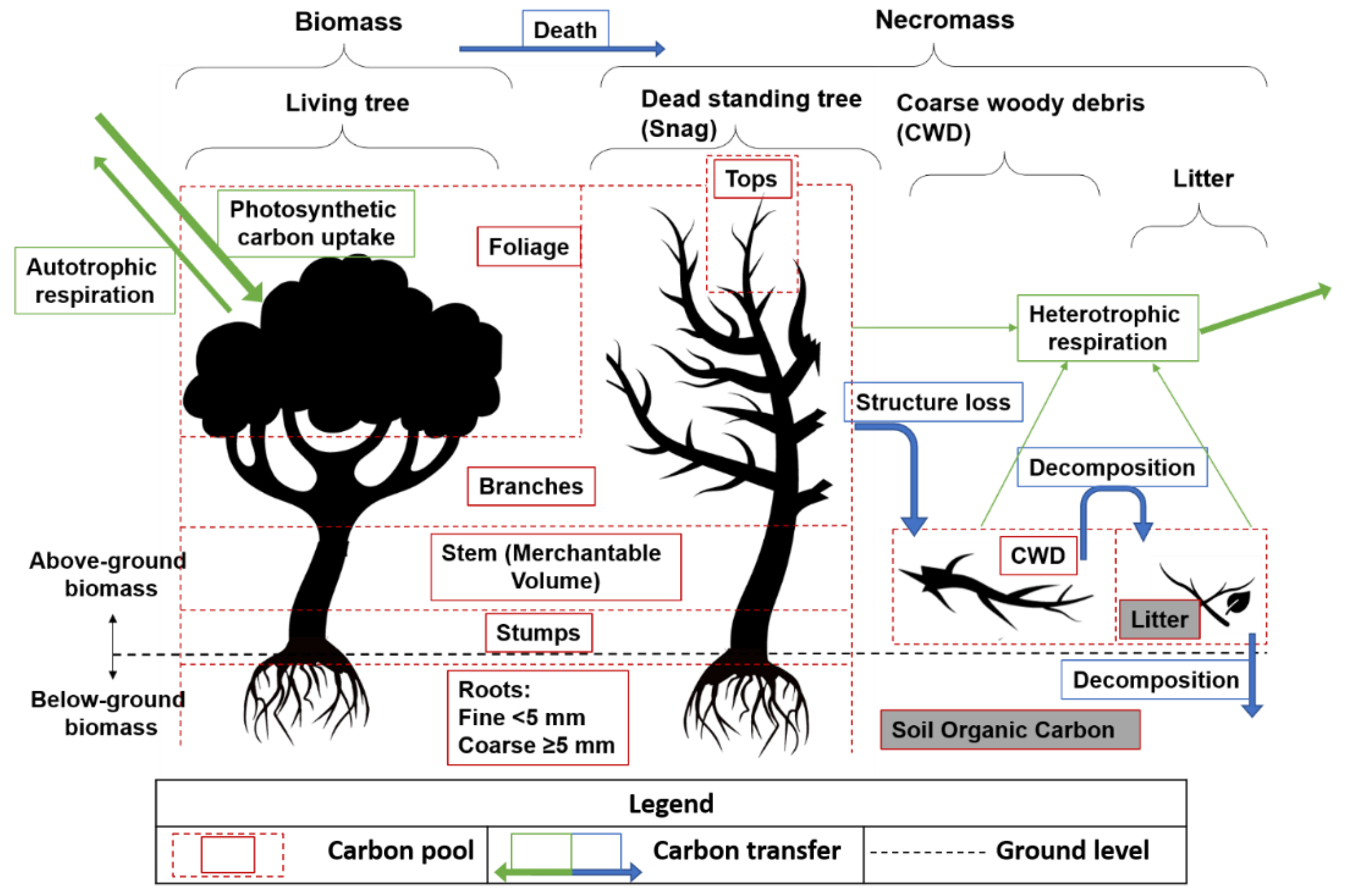
2.3.1. Carbon Calculation from PSP Data

Several methods and equations were used to estimate the various CBM-CFS3 carbon pools from the PSP measurements (Figure 3). All the data processing was completed using R software Version 1.3.1093 [25] and Microsoft (R Core Team: Redmond, WA, USA) Excel version 16.0.13328.20210 [26]. The most recent Nova Scotia PSP data were accessed from the provincial archives, spanning 1965–2019 for living tree measurements and 1998–2019 for coarse woody debris and snag measurements [16]. Using Lambert et al. [6]’s species-specific equations, tree compartment oven-dry biomass was computed from DBH measurements of every tree on every plot (>750,000 individual measurements). Species that did not have a specific equation were reassigned as hardwood or softwood and computed using those generalized equations. The sum of compartment biomass equaled the total above-ground tree biomass, which was used to estimate below-ground (root) biomass using Li et al. [27]’s relationships. Tree biomass measurements (metric tonnes) along with merchantable volume measurements (m3) were summed at the plot level and scaled to per-ha levels.
Tree compartment biomass was first compiled in IPCC-recognized pools to compare measurements against published literature. To assess potential differences in carbon content between forest stand types, plots were assigned a functional group based on the percentage of hardwood or softwood volumes. Plots that contained <75% HW or SW volume by species were assigned a mixedwood functional group [17]. The biomass pools were then multiplied by 0.5 to compute carbon content [1] and then arranged to emulate those pools estimated by the CBM-CFS3 (Figure 3). For the “Merchantable Volume + Bark” (Merch + Bark) pool, the volume of tree tops and stumps were discounted from the total measurement and added to the “Other Volume + Bark” (Other + Bark) pool as per the CBM-CFS3 modelling approach [1] using a Nova Scotia-specific factor of 0.95 [15].
Standing dead tree necromass was calculated from snag measurements using the DBH-based allometric equations and the same scale-up approach. The foliage compartment was subtracted from the total above-ground necromass calculation for dead trees. Coarse woody debris was recorded in the PSPs using the LIM [24] and converted to necromass using the LIM protocol [28]. The USDA species-specific decay reduction and structural loss factors [14] were used to correct the necromass of dead trees and CWD based on their recorded decay level. Nova Scotia uses a three-class decay classification system for standing dead and CWD, which were assigned to their equivalent USDA decay class based on the closest class description (Appendix A Table A1).

Forest Communities

Forest community was chosen as the stratifying variable due to its landscape-level scalability and its ability to differentiate between stands of provincially important tree species and varying carbon accumulation dynamics. Communities were previously delineated using ariel photo interpretation [29]. Communities were selected to explore variance between groups of different species composition, as species exhibit differences in growth dynamics, nutrient regimes, litter, and turnover rates, all of which can affect their carbon dynamics [2]. We chose for this analysis the five most prevalent and significant forest communities in the province, which are comprised of two hardwood-dominated, two softwood-dominated, and one mixed wood forest communities (Table 1). The hardwood functional groups are “HTHw” and “HIHw”, representing tolerant and intolerant hardwood-dominated plots, respectively. Together they account for around 80% of hardwood-dominated plots and cover almost 20% of the Nova Scotia land base. The mixedwood forest community (“MIHwSH”) is comprised of intolerant hardwoods and softwood species. It is the largest mixed wood community and covers almost 20% of the entire PSP dataset. Finally, the softwood functional groups are “SrSbSDom” and “SbFDom” and consist of mostly spruce (red (Picea rubens Sargent.) and black (Picea mariana [Miller] Britton.)) and balsam fir, respectively, both of which are commercially important and cover a substantial portion of the province. Red and black spruce are the province’s largest single forest community, and balsam fir is the third most prevalent softwood species. All other softwood forest communities represent <3% of provincial plots. Combined, the selected forest communities make up almost 67% of the PSP data (Table 1).

Age

Age is a recent addition to the PSP measurement methods, so some older plots do not have an age recording, and some newer plots were missing this recording. To address this, age was back-calculated for all plots based on their most recent age measurement. This was only computed until the plot had a 30% or greater drop in the basal area between successive measurements, at which point the age and forest community were no longer considered accurate, and the older plot measurements were removed from the analysis. Thirty percent is the minimum change in basal area for a stand-altering harvest under Nova Scotia harvest criteria [21]. A change in basal area of this magnitude may therefore indicate a harvest or disturbance that could reset the age or alter the forest community of the stand.
A visual breakdown of the PSP dataset shows a relatively similar distribution of functional groups within age classes except in the 1–20 year age class (Figure 4), indicating biomass was calculated from plots of similar age distributions for each functional group.

2.4. Empirical Model Development

With plots stratified by forest community and assigned an age, 4018 plot measurements were made available for evaluating all relevant CBM-CFS3 carbon pools. Because the Merch + Bark, Other + Bark, Foliage, and Root pools only require living tree data, these individual curves were fit from the entire dataset (1965–2019), totaling over 10,000 plot measurements after age- and community-based omissions. Random subsets of these data were set aside before curve fitting to be used for calculating bias and uncertainty [30]. Datasets were randomly partitioned to produce a subset with a minimum of 100 plots, requiring a < 22% reduction of the least prevalent forest community (balsam fir plots, n = 450) and as little as 7% of the highest represented forest community (SrSbSDom plots, n = 1423).
For these analyses, it was assumed that carbon (t/ha) could be estimated from the stand age (years). Curves were fit with a non-linear least squares (NLS) regression, using R’s nls function [31] to fit the relationship between age (independent variable) and carbon content (dependent variable) for the seven plot-level carbon pools across the five forest communities, resulting in 35 individual relationships produced from the PSP data. The best relationship was the one with the lowest Residual Standard Error. As in many other studies describing tree growth and ecological relationships [32], the scatterplot distributions show a curve shape that can be fitted using either a logistic (1) or power (2) function as follows:
Logistic: Carboni = β1i/(β2i + exp(−β0iX)) + ε,
Power: Carboni = β0i ∗ (X^β1i) + ε,
where: Carbon is the estimated carbon content in t/ha; i is the pool number (i = 1, 2, 3, 4, 5, 6, 7); β0, β1, and β2 are regression parameters that are estimated for each pool; X is the plot age in years; exp is the base of natural logarithms; and ε is an additive error term.
The merchantable volume yield curve was calculated for each plot using a logistic function for each forest community (HIHw, HTHw, MIHwSH, SrSbSDom, SbFDom) as follows:
MerchVoli = β1i/(β2i + exp(−β0iX)) + ε
where: MerchVol is the merchantable volume of the plot in cubic meters; i is the forest community (i = 1, 2, 3, 4, 5); β0, β1, and β2 are regression parameters that are estimated for each community; X is the plot age in years; exp is the base of natural logarithms, and ε is an additive error term.

2.5. Carbon Budget Model of the Canadian Forest Sector

The Carbon Budget Model of the Canadian Forest Sector (CBM-CFS3) uses yield curves relating merchantable volume and stand age to predict past and current carbon stocks and project future stocks as they respond to forest growth and disturbance [33]. It uses equations developed by Boudewyn et al. [34] that describe the stand-level relationship between merchantable volume, age, and above-ground biomass for >60 North American tree species. Boudewyn et al. [34]’s equations relied largely on allometric biomass equations developed by Lambert et al. [6] to estimate the biomass of individual tree compartments based on (a) DBH or (b) DBH and height measurements made on CFS forest plot trees. These equations were calculated for 33 individual Canadian tree species, hardwood, and softwood groupings, as well as all combined species. Equations were fit with data from over 8600 destructive tree samples across Canada, about 20% of which were from the Atlantic provinces. Expansion factors are used to predict non-merchantable biomass in small trees and in non-merchantable components of merchantable trees in the CBM-CFS3 [1]. Below-ground biomass is calculated from the above-ground estimations using Li et al. [27]’s equations, developed from >600 pairs of below- and above-ground biomass measurements from boreal and cold temperate regions.
At every timestep in a CBM-CFS3 simulation, portions of biomass fluctuate between several necromass pools to simulate structure loss/mortality and decomposition. The necromass pools pertinent to this study are “snags” (dead, standing trees) and Medium Dead Organic Matter (Medium DOM) which includes downed dead trees (equivalent to Nova Scotia’s CWD pool) [1]. Temperature-dependent decomposition and transfer rates were compiled from numerous published estimates and National Forest Inventory (NFI) ground plots [15,35].

2.6. CBM-CFS3 Estimations

The CBM-CFS3 simulates many site factors such as disturbance regimes and harvest cycles. This analysis only required the CBM-CFS3 carbon estimation curves computed as a function of the plot age for each forest community. To produce the CBM-CFS3 estimates, we used the CBM-CFS3′s underlying equations (Boudewyn et al. [34] and the same scale-up factors and transfer rates) to compute the carbon pools as an accumulation over time [1,15].
To initiate CWD pools (referred to as the Medium DOM pool in the CBM-CFS3) at year zero, the CBM-CFS3 runs multiple stand life cycles with CWD carbon levels set to increasingly larger values until a “quasi-equilibrium” state is achieved between two consecutive life cycles (see details in [1]). For this analysis, the initial CWD level was set using the equivalent PSP-derived equation at age = zero. Once set, the CBM-CFS3 script estimated carbon as a function of the plot age for each carbon pool under each forest community using only the community-specific merchantable volume curves derived from the PSP measurements.

2.7. PSP Model vs. CBM-CFS3 Estimation Comparison

2.7.1. Pool and Plot-Level Comparison

The CBM-CFS3 estimations (hereafter referred to as the “CBM” method) were compared directly to the empirically derived curves (hereafter referred to as the “PSP” method, curves, or models). The estimations were assessed for uncertainty by calculating their absolute bias and deviation (Root Mean Square Error or RMSE) from the independent subset of data. Uncertainty was compared between pools and between computation methods using the percentages of the mean, i.e., %RMSE (RMSE/mean of observations) and %Bias (Bias/mean of observations). Indeed, %RMSE indicates which method best resembles the independent PSP measurements (i.e., the observations) [36].

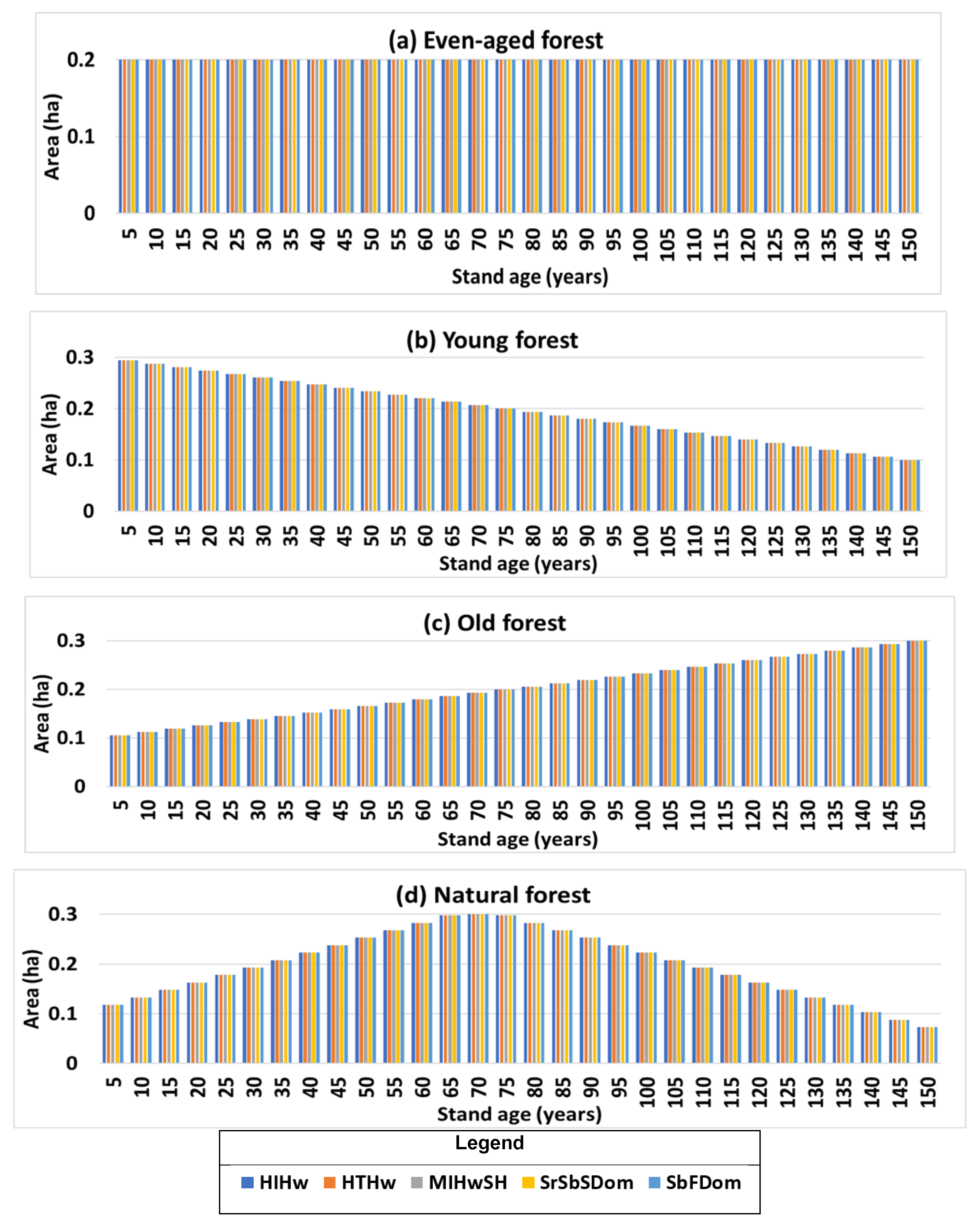
2.7.2. Stand and Landscape-Level Comparison

To assess the implications of choosing one method over the other, the plot-level carbon pool estimations were aggregated to the stand level and estimated over the range of stand ages (1–150 years). The absolute (t/ha) and relative (%) difference of the CBM-CFS3 carbon estimations against PSP carbon estimations were calculated as the mean difference across the age range. The relative difference in carbon estimation was calculated by dividing the absolute difference (CBM estimation—PSP estimation) by the PSP estimation and displayed over the range of plot ages (1–150 years).
Finally, to assess differences between computation methods at the landscape level, following Hennigar et al. [37], a hypothetical 150 ha land base was built containing an even mix of the forest communities used in this analysis. Four age structures were considered: (a) an even mix of the forest communities across all age classes; (b) one skewed towards younger age classes; (c) one skewed towards older age classes; and (d) a scenario in a “natural” age structure, i.e., similar to the Nova Scotia forest [17] (Figure 5a–d). The even-aged landscape (a) can indicate if relative differences between PSP and CBM estimations are reduced from the stand to the landscape level, while scenarios (b) and (c) can display any age-dependent discrepancies in mean absolute carbon estimation. Scenario (d) will show how the models react to a landscape with a natural age structure, where the highest percentage of volume is in middle-aged stands.

3. Results

3.1. Empirical Model Development

Tree biomass compartments and other plot-level biomass measurements (snags and CWD) were aggregated into CBM-CFS3-recognized pools and separated into the five forest communities. Non-linear least squares regressions were used to fit the relationship between these biomasses and the age (X) (Table 2). Of the 35 individual- carbon pool models, 29 were best represented (lowest Residual Standard Error) by a logistic function and six by a power function. The same method was then used to fit the plot-level merchantable volume measurements to age for each forest community (Table 3).

Comparison of Estimations against Independent Observations

Plot-level carbon was then estimated for each forest community as a function of age with the CBM method and the PSP-derived merchantable volume curves and compared against the estimations of the PSP method. Both PSP- and CBM-derived curves were statistically contrasted against the independent PSP datasets (n = 100 per forest community) to assess their congruence with observed data. Bias and Root Mean Square Error (RMSE) totals for all compartments are provided in Appendix B (Table A2 and Table A3). As shown in Figure 6, the RMSE revealed that the highest average error from the observed data was for the Merch + Bark pool, where CBM estimations had an RMSE between 15.9 t/ha for the SbFDom forest community and 24.7 t/ha for the SrSbSDom forest community, while the PSP method estimations had an RMSE between 14.1 and 23.3 t/ha for the same forest communities. The lowest RMSE was usually found in the Fine Root pool, where CBM estimates were on average between 0.7 and 0.8 t/ha different than the observed data and PSP estimations were between 0.5 and 0.8 t/ha different. In all cases, the PSP method had a lower or equal RMSE (and therefore, higher or equal congruence to observed data) than the CBM method, with methods having an equal RMSE in the HTHw (Foliage pool), SbFDom (Fine Root pool), and SrSbSDom (Other + Bark and CWD pools) forest communities.
The Percent RMSE (%RMSE) indicated that the greatest deviation from observed data as a percentage of mean pool carbon was consistently in the CWD and Snag carbon pools (Figure 7), where the highest %RMSE for the PSP method was 126.6% and 123.4% and for the CBM method 132.6% and 125.7%, respectively. For both methods, these extremes were recorded in the HTHw and HIHw forest communities, respectively. In all other pools, the PSP method predicted carbon to within 50% or less of the observed mean except in the SrSbSDom forest community, where the %RMSE was 70.3%, 57.2%, and 74.5% for Merch + Bark, Other + Bark, and Coarse Root pools, respectively. The SrSbSDom Other + Bark and CWD pools were the only instances of the CBM method having a lower %RMSE and therefore higher congruence with observed data than the PSP method: 57.1% vs. 57.2% in Other + Bark respectively, and 104.5% vs. 106.4% in CWD, respectively. In cases where the CBM method has a lower %RMSE, the %RMSE is relatively similar to that of the PSP method, the greatest difference being 1.9%. There are several cases where the PSP method has a %RMSE more than 10% closer to observed data than the CBM method, so taken together, the PSP-derived estimates are more congruent with the observed data.
The bias of the PSP and CBM estimations was computed from the independent, observed data and contrasted between the methods. Bias indicates the level of over- (positive bias) or under- (negative bias) estimation of the models compared to the observed data. Higher bias is shown by a greater distance from zero. When compared to the observed PSP data, the PSP method estimated carbon with a lower bias (closer to zero) than the CBM method in all pools except HTHw Foliage, SbFDom Fine Root, and SrSbSDom Fine Roots (where bias was equal between the methods), as well as in the SbFDom Coarse Root and SrSbSDom Other + Bark and CWD pools (where the PSP method had greater bias than CBM estimations) (Figure 8). Bias was always positive in the Merch + Bark pool, with the PSP average bias ranging between 0.3 to 5.2 t/ha and the CBM average estimations between 1.7 to 9.5 t/ha greater than the observed mean in the HTHw and SrSbSDom forest communities, respectively. In the hardwood and mixed wood forest communities, the CBM method consistently has the highest bias and, therefore, less congruence with the observed data. The CBM method is more likely to overestimate Foliage, Snag, and CWD carbon in the mixed wood and softwood forest communities and more likely to underestimate Coarse and Fine Root carbon in the mixed wood and hardwood forest communities (Figure 8). Several pools show positive bias by one method and negative bias by the other.
Percent bias (%Bias) shows the model bias as a percentage of the observed mean. It allows normalizes the bias for direct comparison between the pools. It shows that the PSP method was more congruent with observations as a percentage of total pool carbon than the CBM method. The PSP method only has one instance of bias >20%: in the SrSbSDom CWD pool, where its predictions are 22% less (negative bias) than the mean observed carbon in that pool (Figure 9). More than half of the CBM estimations have greater than 20% bias (both positive and negative) compared to the observed means, with seven pools being predicted with >40% bias: HTHw Snag (−61%); MIHwSH Other + Bark (46.9%), and Foliage (47.6%); SbFDom Other + Bark (−42.4%), Foliage (55%), and Snag (45.9%); and SrSbSDom Foliage (53.9%).
The PSP method estimates tend to be greater than the observed data (positive %Bias) but consistently underestimate the CWD pool across all forest communities (negative %Bias) (Figure 9). The CBM estimates had greater %Bias than PSP estimates in all cases except HTHw (Foliage), SbFDom (Coarse Root), and SrSbSDom (Other + Bark) pools. The CBM estimates were more likely to under-predict carbon when compared to the observed data (negative %Bias), especially in the hardwood and mixed wood forest communities, and tend to overpredict (positive %Bias) Foliage, Snag, and CWD in the mixed wood and softwood forest communities.

3.2. Stand-Level Method Comparison

Aggregating plot-level carbon estimations to the stand scale revealed differences in method estimation based on forest community and age. Estimation methods have relatively stable congruence after the approximate age of 50, remaining more consistent (±<15%) for the rest of the estimation period (Figure 10). In the youngest stands, the hardwood and mixed wood forest communities are overestimated by the CBM-CFS3 (positive relative difference) when compared to the PSP method, with congruence increasing with age. The carbon in these three forest communities was initially overestimated by the CBM method by between 40–55%, a difference that gradually decreases and stabilizes to <20%. The softwood communities had a more complicated congruence pattern over time. The difference in CBM carbon estimation in the SbFDom community initially increased from near zero to a 24% overestimation around age twelve, at which point the difference decreases, becomes negative (CBM begins underestimating carbon compared to the PSP method), then gradually increased again to become consistent at a near-zero difference around age 50 (Figure 10). In the SrSbSDom community, the CBM method underestimated carbon by over 40% at age one compared to PSP estimates, a difference that converges on zero, diverges, then converges again to less than −20% around age 50, and steadies at <10% as stands near age 90.
When mean differences were compared over the entire length of the simulation (the mean over 150 years), the equations were most similar in predicting SbFDom at the stand level (mean difference of −2.2 t/ha) and least congruent when predicting spruce stands (SrSbSDom, mean difference of −8.4 t/ha) (Table 4). The relative difference ranged from −3.1% to −17.6%, again in the SbFDom and SrSbSDom forest communities, respectively. Mean CBM estimates were higher than PSP estimates in all hardwood and mixed wood stand types (indicated by positive differences), whereas carbon predictions in softwood stands were lower using the CBM method (negative differences) (Table 4).

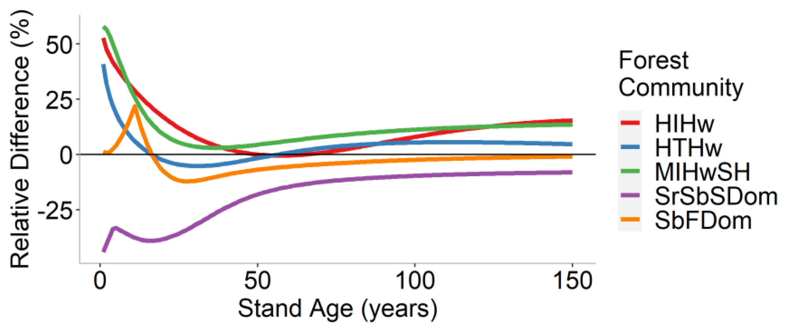
3.3. Landscape-Level Method Comparison

At the landscape level, the absolute difference in carbon estimation varied over time depending on the age class structure, with the CBM method overestimating carbon in the youngest and oldest stands and underestimating stands aged 20–70 across all age-structure scenarios (Figure 11). The CBM method overestimated carbon in young stands to a greater extent in the young-skewed scenario (b) and in older stands in the old-skewed forest (c), with the difference in even (a) and natural (d) scenarios generally falling in between (b) and (c) across most age classes.
When aggregated to the landscape level, relative differences in estimation between PSP and CBM methods were reduced. The CBM method overestimated (positive % difference) landscape-level carbon by 26% at age one when compared to the PSP estimations (Figure 12). The differences are quickly reduced as the stand age, becoming near zero by age 20, at which point the CBM estimations become less than the PSP estimations, nearing 7% less by age 30. Congruence increases again after age 30, nearing zero around age 70. The CBM overestimates again for the remainder of the planning horizon, estimating 6.3% more carbon on the landscape by age 150 (Figure 12).
When the mean carbon estimation over the entire planning horizon was compared, the scenario with even-aged stands (Scenario a) had a mean difference of 8.4 t/ha of carbon, meaning the CBM method estimated 2.4% more carbon on the landscape than the PSP method (Table 5). The relative difference remained the same for the young, old, and natural forest scenarios (scenarios b, c, and d respectively), but scenarios b and d have a lower difference in actual carbon estimated on the landscape (5 t/ha) and scenario c had a higher mean estimation difference (11.8 t/ha) (Table 5).

4. Discussion

This study calculated localized carbon estimation models from PSP tree measurements and compared them to estimations of the CBM-CFS3 at the plot, stand, and landscape levels. Results indicate that the implications of using the localized, PSP-derived models over the CBM-CFS3 method change depending on (a) the scale at which the estimations are being made; (b) the carbon pools being estimated (when estimating at the compartment- or plot-scale), and (c) the age and species composition of the stand or landscape to be estimated. Most empirical models are calculated at the compartment and plot level, where measurements are taken, while carbon projects and planning initiatives are often estimated at the stand or landscape level as these projects require large areas to be feasible [38]. Our results indicate that the national-scale CBM-CFS3 has utility even at fine spatial scales and suggest that the localized PSP-derived models behave reasonably when scaled up to the landscape level. The implications of altering other variables are discussed in the context of each scale.

4.1. Tree and Plot-Level Biomass

The Merch + Bark pool showed the highest levels of total RMSE and bias when compared to the observed PSP dataset, which was expected as this is the largest carbon pool. The %RMSE and %Bias results were better indicators of estimation congruence to observed data when comparing between carbon pools. These results suggest the PSP-derived carbon estimation curves better reflect the observed Nova Scotia PSP forest measurements than the CBM estimates as they generally have a lower %RMSE at the pool level. Several pools are predicted by the CBM method with a lower %RMSE than the PSP curves. Researchers can consider this when the goal is to estimate these carbon pools in isolation for pool-specific research.
The highest error for both methods occurred in the Snag and CWD estimates, which could result from fewer data or more variability within these pools as they have only been measured in PSPs since the late 1990s. It is also likely be influenced by the difference in estimation methods for these two necromass pools. In both methods, merchantable volume, foliage, and root biomass pools were directly estimated by the same equations and expansion factors, whereas the CBM-CFS3 estimations of CWD relied on additional biomass turnover rates and litterfall assumptions [1] and are being compared to models derived from direct PSP measurements of this pool. Moreover, the spin-up and initiation of carbon storage values in necromass pools in CBM-CFS3 based on assumed disturbance histories are highly influential on CWD and snag dynamics.
Bias indicates the extent to which the estimation methods over- or underpredict pool-level carbon when compared to the observed data, so these results can be considered when choosing a method to estimate individual carbon pools in isolation. Overestimation of carbon can have negative environmental and financial consequences, and carbon accounting protocols generally require conservative estimates or discounted pay-outs proportional to the uncertainty [4]. Although the PSP method has %Bias closer to zero in most pools, it may be more appropriate to use the CBM method when the CBM method has negative %Bias and the PSP method has positive %Bias avoid overestimation.
The error of estimation (RMSE) was calculated against the independent observed dataset, but other types of error propagate in the calculation process. These include the estimation error of individual models used to estimate carbon (e.g., allometric equations, carbon fraction calculation, and above- to below-ground extrapolation) and sampling error. To fully understand the quality of the empirical carbon estimation models produced in this analysis, a full investigation of errors in the calculation process should be conducted to determine how it affects the final output.

4.2. Stand- and Landscape-Level Comparison

Carbon estimation between methods was least congruent in young stands, with estimations becoming more congruent with advancing stand age. This could be caused by fewer observations [39] or higher structural variability in young stands. Several studies suggest compartment-level models can be “forced through the origin” (Carbon = zero at Age = zero) to better reflect “real-world” conditions of living biomass [40]. This study chose instead to use the functions that best fit the PSP dataset across all year ranges in order to compute the best-fitting model for the overall age range. When a natural plot is harvested or disturbed to the extent that age is reset to zero, it could contain varying regeneration and/or retention levels. Disturbance can leave debris and different soil conditions depending on type and intensity, all of which can affect stand development [41]. Thus, forcing functions through the origin may be more acceptable for planted stands with better-defined starting age. As shown, differences at the compartment- and plot-level were reduced when scaled up. The Nova Scotia State of the Forest report [17] states that most provincial forest plots are in 40–80-year-old age classes, and results suggest that increasing the proportion of these age classes in the analysis would increase the congruence of estimations.
The SrSbSDom (spruce-dominated) forest community had the most pronounced estimation differences, with the CBM-CFS3 underestimating spruce stand carbon by 30%–40% in stands aged <20 years and by >17% overall when compared to the PSP curves (Figure 10 and Table 4). Just like in Nova Scotia, the Canadian national forest is spruce-dominated [42]. Most of these spruce stands reside in the boreal and western regions, so CBM-CFS3 spruce assumptions that are based on the national inventory may be biased away from the unique Acadian spruce forests that are dominated by red spruce on zonal sites. Even those assumptions based on specific Atlantic Maritime Ecozone information would include New Brunswick, an inland spruce-dominated forest that is physically closer to the boreal forest [15]. As this is one of the predominant forest communities in Nova Scotia, these results should be considered when modelling spruce stands and is an area where the CBM-CFS3 could benefit from more Acadian forest-specific empirical data.
Mean relative differences between forest communities suggest that, over the 150-year planning horizon, the CBM method overestimates hardwood and mixed wood community types and underestimates softwood community types when compared to the PSP method (Table 4). The Nova Scotia landscape consists of over 50% softwood stand types, with increasing levels of hardwood stands every year [17]. Stand-level analysis suggests that increasing levels of young spruce stands in the analysis will cause the CBM-CFS3 estimations to become less congruent with PSP curves, and if combined with the full breadth of stand ages, will make the CBM method more likely to underestimate landscape-level carbon by comparison. Increased levels of young stands of hardwood and mixedwood forest communities will make the CBM method more likely to overestimate carbon when compared to the PSP method.
At the landscape level, the mean absolute difference is lowest in the young-skewed and natural landscapes (5.0 t/ha, Table 5) because the lower ages (<70 years) have a mixture of over-and under-predictions (Figure 11) that result in a more balanced mean. The old-skewed forest has the highest mean difference because the differences are exclusively >0 over the age of 70, with no negatives to counteract the positives. The CBM-CFS3 predicts landscape-level carbon to within 2.4% of the localized PSP models, which is relatively close when compared to the plot and stand-level analysis. This result aligns with various studies that found increasing the spatial scale of models can reduce the uncertainty of their individual structures [43]. Implications for forest research and management consequently depend on the activity scale. For landscape-level management planning (such as provincial wood supply or provincial carbon reporting), results would be comparable between the CBM and the PSP method, the latter being 2.4% more conservative. When estimating carbon at the compartment, plot, or stand level for research or smaller reporting initiatives, more consideration is needed when choosing one method over the other. The PSP method generally showed more congruence to observed data, but if conservative estimations are required (as they often are for carbon markets), the CBM method may be more appropriate for predicting the plot-level carbon pools where it displayed negative bias.

4.3. Further Considerations

Results also suggest areas of focus to improve data collection regimes for carbon modeling purposes. In most cases, the CBM-CFS3 estimated individual carbon pools with less agreement to observed Nova Scotia PSP data when compared to the PSP-derived curves. The inclusion of more Nova Scotia-specific plot data could therefore improve CBM-CFS3 algorithms for the area (as well as improving the local PSP-derived curves), most notably in pools with higher %RMSE and %Bias such as the Snag and CWD pools (Figure 7 and Figure 9 respectively) and in stand types/ages with low estimation congruence between methods (such as young SrSbSDom stands). In addition, some areas of uncertainty were identified as follows:
  • The 50% carbon assumption. The CBM-CFS3 assumes a 50% carbon ratio to oven-dried biomass, consequently used in this analysis. This general rule is not valid when looking at individual tree tissues or individual species, as softwood trees often contain slightly greater than 50% carbon content and hardwood species slightly below 50% [44]. Local estimations could therefore be improved if species- and tissue-specific carbon ratios were used.
  • Forest community classification. The use of remote sensing data (i.e., aerial photography) to classify forest communities was chosen as this is how the NSDLF classifies stands for management planning. As the PSP data offers a breakdown of species composition for every plot, it would be possible to classify stands based on the percent composition of species, which could reduce the error associated with remotely- sensed classification. Moreover, the Boudewyn et al. [34] equations rely on a single leading species to be used when converting merchantable volume to biomass at the stand level, which may further explain some of the differences in the results of this study. Forest community was a broad enough classification to maintain large sample sizes post-stratification. Other variables considered included land capability, which is often used in forest models as an indicator of site quality. The land capability was not used here as it is a derivative of age, and therefore could be confounding in this analysis where age is necessary to compare against CBM-CFS3 output. It would also further reduce sample sizes between groups. Site index or other types of site-describing variables that influence forest growth and yield were not included in this analysis, which is a limitation of this study and an area for future research. However, the reason for not having the site in the regression analysis was because this study aimed to compare empirical models to the CBM-CFS3 model at multiple scales as parsimoniously as possible. The purpose was not to develop the most accurate predictions and yield curves for carbon or merchantable volume. This was also why merchantable volume curves were developed from the same PSP data as were used for carbon and the existing NSDLF yield curves (which include several site metrics) were not used.
  • Age. Age is a subjective variable to assess natural forests, especially in more mature or uneven-aged stands, but it is necessary in this analysis for CBM-CFS3 comparison. This analysis assumes forest stands are a uniform age when actual forest stands can contain several cohorts of trees and variable mortality. Forest plots can be difficult to assign an age to; they can maintain different levels of regeneration even after disturbance or harvest resets the age to zero. A protocol should be established to apply these methods to stands of varying successional stages. Moreover, Nova Scotia is moving towards a model of forestry that relies more on partial harvests with multi/all-aged silviculture systems, which will further challenge the prominent use of stand age in forest (and forest carbon) modelling.

5. Conclusions

This analysis did not intend to identify one method of carbon estimation as superior but rather to compare the methods and offer insight into their differences. As shown here, the implications of using one method over the other change depending on the scale and specific variables to be estimated and the desired function of the results. In most cases, the locally derived carbon estimation models performed with more congruence to observed data than the CBM method at the plot scale, but the underestimation of the CBM-CFS3 may be desirable when estimating the environmental benefits of a carbon project. At the landscape level, the CBM-CFS3 predicted carbon to be within 2.4% of the local models.
The differences in estimation highlight the importance of assessing large generic models with local data. The similarities demonstrate the utility of large-scale models even in some smaller localized settings while simultaneously improving our understanding of the local model performance when scaled up, where results indicate a similar performance to the nationally accepted CBM-CFS3. This difference across scales and variables can offer researchers some insight when selecting a method for specific modeling applications and can reveal opportunities to improve the function of both the local models and the CBM-CFS3.

Author Contributions

Conceptualization, J.S. and J.H.; methodology, J.S. and J.H.; software, J.S. and J.H.; validation, J.S.; formal analysis, J.S. and J.H.; resources, J.S. and J.H.; data curation, J.S.; writing—original draft preparation, J.H.; writing—review and editing, B.L. and J.S.; visualization, J.S.; supervision, B.L. and J.S.; project administration, B.L. and J.S. All authors have read and agreed to the published version of the manuscript.

Funding

This research received no external funding. The Nova Scotia Department of Lands and Forestry provided in-kind support in the forest of data and staff time.

Institutional Review Board Statement

Not applicable.

Informed Consent Statement

Not applicable.

Data Availability Statement

The photo-interpreted forest inventory data from Nova Scotia are publicly available at the following location: https://novascotia.ca/natr/forestry/gis/forest-inventory.asp (accessed on 1 September 2019). The Nova Scotia Department of Lands and Forestry permanent sample plot data are not publicly available for immediate download because the plots are located across all land ownership types and have associated privacy concerns. Instead, individuals can contact the Department and arrange for a data-sharing agreement in order to access the data for research purposes.

Acknowledgments

The authors would like to thank Jürgen Bauhus (Albert-Ludwigs University of Freiburg, Germany) for his contributions to and co-supervision of this project. We also thank the resource analysis staff and forest inventory staff at the Nova Scotia Department of Lands and Forestry for their input on forest data and modeling. This study has been reviewed by the Forestry Division of the Nova Scotia Department of Lands and Forestry and approved for publication. Approval does not signify that the contents reflect the views of the Department, nor does mention of trade names or commercial products constitute endorsement or recommendation for use.

Conflicts of Interest

The authors declare no conflict of interest.

Appendix A. Decay Classes

Table A1. Nova Scotia (NS) decay class number and description for standing dead or snags and coarse woody debris (CWD) [45] and their equivalent USDA classes [14] *. This Table was created for this study, the text is a direct quotation from the Nova Scotia Department of Lands and Forestry [45] and USDA Forest Service [14].
Nova Scotia USDA
Number SnagsCWDNumberSnagsCWD
1Recently Dead. Branches and twigs intact, bark on.Bark on, hard bole, round, twigs and branches present and supporting log partially off the ground.1All limbs and branches are present; the top of the crown is still present; all bark remains; sapwood is intact, with minimal decay; heartwood is sound and hard.Sound, freshly fallen, intact logs with no rot, no conks present indicating a lack of decay, original wood color, no invading roots, fine twigs attached with tight bark.
2Moderate decay. Dead for a number of years, shedding fine twigs and branches, bark loose and flaking, fairly sound/wind firm, bole has signs of decay/rot in sapwood or heartwood that was sound at the time of mortality.Bark flaking, mostly hard bole (little decay), round, few branch stubs, flat on the ground.3Only limb stubs exist; the top is broken; a variable amount of bark remains; sapwood is sloughing; heartwood has advanced decay in upper bole and is beginning at the base.Heartwood is still sound with piece supporting its own weight, sapwood can be pulled apart by hand or is missing, wood color is the reddish-brown or original color, roots may be invading sapwood, only branch stubs are remaining which cannot be pulled out of the log.
3Advanced Decay. Decay/rot in bole is advanced, most of the bark being flaking off or absent, the stability is declining.Bark mostly gone, soft bole, oval, sinking into the ground.4Few or no limb stubs remain; the top is broken; a variable amount of bark remains; sapwood is sloughing; heartwood has advanced decay at the base and is sloughing in the upper bole.Heartwood is rotten with pieces unable to support own weight, rotten portions of the piece are soft and/or blocky in appearance, a metal pin can be pushed into heartwood, wood color is reddish or light brown, invading roots may be found throughout the log, branch stubs can be pulled out.
5No evidence of branches remains; the top is broken; <20 percent of the bark remains; sapwood is gone; heartwood is sloughing throughout.There is no remaining structural integrity to the piece with a lack of circular shape as rot spreads out across the ground, the rotten texture is soft and can become powder when dry, wood color is red-brown to dark brown, invading roots are present throughout, branch stubs and pitch pockets have usually rotten down.
* Nova Scotia Decay Class 3 is equivalent to both USDA Class 4 and 5, so NS Class 3 necromass records were corrected using the average coefficients between USDA Class 4 and 5.

Appendix B. Root Mean Square Error and Bias

Table A2. Root Mean Square Error (RMSE) and Percent RMSE of both estimation methods against an independent PSP dataset (n = 100 per community) by forest community and carbon pool.
Forest CommunityCarbon PoolRMSE (t/ha)% RMSE
PSPCBMPSPCBM
HIHwMerch + Bark19.32148.152.4
Other + Bark7.29.444.257.7
Coarse Roots4.65.145.250.6
Fine Roots0.50.834.649.3
Foliage1.72.248.961.7
Snags4.95.0123.4125.7
CWD2.32.585.793.6
HTHwMerch + Bark16.316.427.928.1
Other + Bark6.06.726.329.3
Coarse Roots3.65.028.840.0
Fine Roots0.50.733.645.8
Foliage1.41.442.143.2
Snags4.55.298.3115.3
CWD4.74.9126.6132.6
MIHwSHMerch + Bark17.118.046.748.9
Other + Bark7.210.347.167.1
Coarse Roots4.25.345.757.7
Fine Roots0.70.845.054.4
Foliage2.02.947.267.5
Snags4.64.880.583.5
CWD4.44.5111.4113.2
SbFDomMerch + Bark14.115.948.354.6
Other + Bark5.97.948.664.8
Coarse Roots3.53.448.246.0
Fine Roots0.80.850.251.6
Foliage2.53.948.473.9
Snags4.24.977.989.4
CWD3.73.893.995.5
SrSbSDomMerch + Bark23.324.770.374.3
Other + Bark6.56.557.257.1
Coarse Roots6.36.574.576.1
Fine Roots0.70.748.449.6
Foliage2.43.352.874.3
Snags4.04.478.286.7
CWD2.72.7106.4104.5
Table A3. Bias and Percent Bias of both estimation methods against an independent PSP dataset (n = 100 per community), by forest community and carbon pool.
Forest CommunityCarbon PoolBias% Bias
PSPCBMPSPCBM
HIHwMerch + Bark2.99.07.222.4
Other + Bark0.4−5.82.2−35.8
Coarse Roots0.7−2.16.7−20.7
Fine Roots0.1−0.45.0−23.1
Foliage0.21.36.636.3
Snags0.0−0.10.0−2.6
CWD−0.3−1.0−11.2−39.2
HTHwMerch + Bark0.31.70.42.9
Other + Bark−0.41.8−1.87.9
Coarse Roots0.0−3.4−0.1−27.1
Fine Roots0.0−0.5−2.7−30.3
Foliage0.10.12.72.4
Snags−0.7−2.8−16.1−61.0
CWD−0.4−0.7−9.7−18.8
MIHwSHMerch + Bark1.25.23.214.2
Other + Bark1.5−7.29.6−46.9
Coarse Roots0.2−3.32.6−36.0
Fine Roots0.0−0.42.1−27.7
Foliage0.32.17.447.6
Snags0.31.34.723.0
CWD0.41.011.124.9
SbFDomMerch + Bark4.28.414.429.0
Other + Bark0.2−5.11.4−42.4
Coarse Roots1.10.015.10.5
Fine Roots0.1−0.18.9−9.7
Foliage0.42.98.255.0
Snags 2.55.745.9
CWD 1.0−12.425.2
SrSbSDomMerch + Bark5.29.515.728.7
Other + Bark0.60.55.54.3
Coarse Roots1.5217.923.5
Fine Roots0.2−0.211.1−15.2
Foliage0.62.414.453.9
Snags−0.21.8−4.936.0
CWD−0.60.4−22.516.4

References

  1. Kurz, W.A.; Dymond, C.C.; White, T.M.; Stinson, G.; Shaw, C.H.; Rampley, G.J.; Smyth, C.; Simpson, B.N.; Neilson, E.T.; Trofymow, J.A.; et al. CBM-CFS3: A model of carbon-dynamics in forestry and land-use change implementing IPCC standards. Ecol. Model. 2009, 220, 480–504. [Google Scholar] [CrossRef]
  2. Eggleston, S.; Buendia, L.; Miwa, K.; Ngara, T.; Tanabe, K. IPCC Guidelines for National Greenhouse Gas. Inventories; Intergovernmental Panel on Climate Change; Institute for Global Environmental Strategies: Hayama, Japan, 2006; Volume 5. [Google Scholar]
  3. Gibbs, H.K.; Brown, S.; Niles, J.O.; Foley, J.A. Monitoring and estimating tropical forest carbon stocks: Making a reality. Environ. Res. Lett. 2007, 2, 45023. [Google Scholar] [CrossRef]
  4. Hamburg, S. Simple rules for measuring changes in ecosystem carbon in forestry-offset projects. Mitig. Adapt. Strateg. Glob. Chang. 2000, 5, 25–37. [Google Scholar] [CrossRef]
  5. Brown, S. Estimating Biomass and Biomass Change of Tropical Forests: A Primer; FAO Forestry Paper-134; Food and Agriculture Organization of the United Nations: Rome, Italy, 1997. [Google Scholar]
  6. Lambert, M.-C.; Ung, C.; Raulier, F. Canadian national tree above-ground biomass equations. Can. J. For. Res. 2005, 35, 1996–2018. [Google Scholar] [CrossRef]
  7. Stark, H.; Nothdurft, A.; Bauhus, J. Allometries for Widely Spaced Populus ssp. and Betula ssp. in Nurse Crop Systems. Forests 2013, 4, 1003–1031. [Google Scholar] [CrossRef]
  8. Suchomel, C.; Pyttel, P.; Becker, G.; Bauhus, J. Biomass equations for sessile oak (Quercus petraea (Matt.) Liebl.) and hornbeam (Carpinus betulus L.) in aged coppiced forests in southwest Germany. Biomass Bioenergy 2012, 46, 722–730. [Google Scholar] [CrossRef]
  9. Mokany, K.; Raison, R.J.; Prokushkin, A.S. Critical analysis of root: Shoot ratios in terrestrial biomes. Glob. Chang. Biol. 2006, 12, 84–96. [Google Scholar] [CrossRef]
  10. Paul, K.I.; Roxburgh, S.H.; Chave, J.; England, J.R.; Zerihun, A.; Specht, A.; Lewis, T.; Bennett, L.T.; Baker, T.G.; Adams, M.A.; et al. Testing the generality of above-ground biomass allometry across plant functional types at the continent scale. Glob. Chang. Biol. 2016, 22, 2106–2124. [Google Scholar] [CrossRef] [PubMed]
  11. Chen, W.; Zhang, Q.; Cihlar, J.; Bauhus, J.; Price, D. Estimating fine-root biomass and production of boreal and cool temperate forests using above-ground measurements: A new approach. Plant. Soil 2004, 265, 31–46. [Google Scholar] [CrossRef]
  12. Penman, J.; Gytarsky, M.; Hiraishi, T.; Krug, T.; Kruger, D.; Pipatti, R.; Buendia, L.; Miwa, K.; Ngara, T.; Tanabe, K.; et al. Good practice guidance for land use, land-use change and forestry. In Good Practice Guidance for Land Use, Land-Use Change and Forestry; IPCC Institute for Global Environmental Strategies: Kanagawa, Japan, 2003. [Google Scholar]
  13. Domke, G.M.; Woodall, C.W.; Smith, J.E. Accounting for density reduction and structural loss in standing dead trees: Implications for forest biomass and carbon stock estimates in the United States. Carbon Balance Manag. 2011, 6, 14. [Google Scholar] [CrossRef] [PubMed] [Green Version]
  14. Harmon, M.; Woodall, C.; Fasth, B.; Sexton, J.; Yatkov, M. Differences between Standing and Downed Dead Tree Wood Density Reduction Factors; Res. Pap. NRS-15. U.S. Department of Agriculture, Forest Service, Northern Research Station: Newtown Square, PA, USA, 2011; 40p. Available online: https://permanent.access.gpo.gov/gpo14619/rp-nrs15.pdf (accessed on 10 August 2020).
  15. Kull, S.; Rampley, G.; Morken, S.; Metsaranta, J.; Neilson, E.; Kurz, W. Operational-Scale Carbon Budget Model of the Canadian Forest Sector (CBM-CFS3) Version 1.2: User’s Guide; Canadian Forest Service; Norther Forestry Centre: Edmonton, AB, Canada, 2019; 348p. [Google Scholar]
  16. NSDNR. Nova Scotia Data File: Inventory Permanent Sample Plots Data; Department of Lands and Forestry: Truro, NS, Canada, 2019; Available for research purposes upon request of the Department. [Google Scholar]
  17. NSDNR. State of the Forest Report; Department of Lands and Forestry: Truro, NS, Canada, 2016; 90p, Available online: https://novascotia.ca/natr/forestry/reports/State_of_the_Forest_2016.pdf (accessed on 15 August 2020).
  18. Metsaranta, J.M.; Shaw, C.H.; Kurz, W.A.; Boisvenue, C.; Morken, S. Uncertainty of inventory-based estimates of the carbon dynamics of Canada’s managed forest (1990–2014). Can. J. For. Res. 2017, 47, 1082–1094. [Google Scholar] [CrossRef]
  19. Environment and Climate Change Canada. Environment Canada Weather Records, Nova Scotia Average Temperature. 2020. Available online: https://climate.weather.gc.ca/historical_data/search_historic_data_e.html?hlyRange=1960-10-01%7C1986-12-31&dlyRange=1960-10-01%7C2002-10-31&mlyRange=1960-01-01%7C2002-10-01&urlExtension=_e.html&searchType=stnProv&optLimit=yearRange&StartYear=1980&EndYear=2020&selRowPerPage=25&Line=186&Month=12&Day=7&lstProvince=NS&timeframe=3&Year=2002 (accessed on 4 May 2020).
  20. Wein, R.W.; Speer, J.E. Lichen Biomass in Acadian and Boreal Forests of Cape Breton Island, Nova Scotia. Bryologist 1975, 78, 328–333. Available online: http://www.jstor.org/stable/3241889 (accessed on 15 August 2020). [CrossRef]
  21. McGrath, T. Nova Scotia Forest Management Guide; FRR # 100, Report FOR 2018-001; Department of Lands and Forestry: Truro, NS, Canada, 2018; 158p. [Google Scholar]
  22. Canada’s National Forest Inventory Website. Available online: https://nfi.nfis.org/en/maps (accessed on 15 July 2020).
  23. Townsend, P. Nova Scotia Forest Inventory Based on Permanent Sample Plots Measured between 1999 and 2003; Report FOR 2004-3; Department of Natural Resources, Forestry Division: Truro, NS, Canada, 2004; 31p. [Google Scholar]
  24. NSDNR. Forest Inventory Permanent Sample Plot Field Measurement Methods and Specifications; Nova Scotia Department of Natural Resources, Forestry Division: Truro, NS, Canada, 2004; 66p, Available online: https://novascotia.ca/natr/forestry/reports/InvReport2004.pdf (accessed on 5 September 2021).
  25. R Core Team. R: A Language and Environment for Statistical Computing, version 1.3.1093; R Core Team: 2019. Available online: https://www.r-project.org/ (accessed on 1 March 2020).
  26. Microsoft Core Team. Excel Version 16.0.13328.20210; Microsoft Corporation: Redmond, WA, USA, 2019. [Google Scholar]
  27. Li, Z.; Kurz, W.A.; Apps, M.J.; Beukema, S.J. Belowground biomass dynamics in the Carbon Budget Model of the Canadian Forest Sector: Recent improvements and implications for the estimation of NPP and NEP. Can. J. For. Res. 2003, 33, 126–136. [Google Scholar] [CrossRef]
  28. Marshall, P.L.; Davis, G.; LeMay, V.M. Using Line Intersect Sampling for Coarse Woody Debris; Technical Report TR-003; BC Ministry of Forests, Nanaimo Research Section, Vancouver Forest Region: Vancouver, BC, Canada, 2000; 34p. [Google Scholar]
  29. Nova Scotia Data File: Crown Land Forest Model Data; Department of Lands and Forestry: Truro, NS, Canada, 2019.
  30. Harrel, F. Regression Modeling Strategies: With Applications to Linear Models, Logistic and Ordinal Regression, and Survival Analysis; Springer: New York, NY, USA, 2015; Volume 3, pp. 72–114. [Google Scholar]
  31. Florent, B.; Christian, R.; Sandrine, C.; Martin, B.; Jean-Pierre, F.; Marie-Laure, D.-M. A Toolbox for Nonlinear Regression in R: The Package nlstools. J. Stat. Softw. 2015, 66, 1–21. Available online: http://www.jstatsoft.org/v66/i05/ (accessed on 1 March 2020).
  32. Fekedulegn, D.; Mac Siurtain, M.P.; Colbert, J.J. Parameter estimation of non-linear growth models in forestry. Silva. Fenn. 1999, 33, 327–336. Available online: https://www.researchgate.net/publication/241321199_Parameter_Estimation_of_Nonlinear_Growth_Models_in_Forestry (accessed on 15 August 2020). [CrossRef] [Green Version]
  33. Stinson, G.; Kurz, W.A.; Smyth, C.E.; Neilson, E.T.; Dymond, C.C.; Metsaranta, J.M.; Boisvenue, C.; Rampley, G.J.; Li, Q.; White, T.M.; et al. An inventory-based analysis of Canada’s managed forest carbon dynamics, 1990 to 2008. Glob. Chang. Biol. 2011, 17, 2227–2244. [Google Scholar] [CrossRef] [Green Version]
  34. Boudewyn, P.; Song, X.; Magnussen, S.; Gillis, M.D. Model-Based, Volume-to-Biomass Conversion for Forested and Vegetated Land in Canada; Information Report BC-X-411; Canadian Forest Service, Pacific Forestry Centre: Victoria, BC, Canada, 2007; 112p. [Google Scholar]
  35. Moroni, M.T.; Shaw, C.H.; Kurz, W.A.; Rampley, G.J. Forest carbon stocks in Newfoundland boreal forests of harvest and natural disturbance origin II: Model evaluation. Can. J. For. Res. 2010, 40, 2146–2163. [Google Scholar] [CrossRef]
  36. Vorster, A.; Evangelista, P.H.; Stovall, A.E.L.; Ex, S. Variability and uncertainty in forest biomass estimates from the tree to landscape scale: The role of allometric equations. Carbon Balance Manag. 2020, 15, 1–20. Available online: https://cbmjournal.biomedcentral.com/articles/10.1186/s13021-020-00143-6#citeas (accessed on 19 August 2020). [CrossRef]
  37. Hennigar, C.R.; MacLean, D.A.; Amos-Binks, L.J. A novel approach to optimize management strategies for carbon stored in both forests and wood products. For. Ecol. Manag. 2008, 256, 786–797. [Google Scholar] [CrossRef]
  38. Seeberg-Elverfeldt, C. Carbon Finance Possibilities for Agriculture, Forestry and Other Land Use Projects in a Smallholder Context; Food and Agriculture Organization of the United Nations: Rome, Italy, 2010. [Google Scholar]
  39. Picard, N.; Bosela, F.B.; Rossi, V. Reducing the error in biomass estimates strongly depends on model selection. Ann. For. Sci. 2015, 72, 811–823. [Google Scholar] [CrossRef] [Green Version]
  40. Kozak, A.; Kozak, R.A. Notes on regression through the origin. For. Chron. 1995, 71, 326–330. [Google Scholar] [CrossRef] [Green Version]
  41. Reyes, G.P.; Kneeshaw, D.; Grandpré, L.D.; Leduc, A. Changes in woody vegetation abundance and diversity after natural disturbances causing different levels of mortality. J. Veg. Sci. 2010, 21, 406–417. Available online: http://www.jstor.org/stable/40925497 (accessed on 12 August 2020). [CrossRef]
  42. Power, K.; Gillis, M.D. Canada’s Forest Inventory 2001–2006; Information Report BC-X-408E; Canadian Forest Service, Pacific Forestry Centre: Victoria, BC, Canada, 2006; 100p. [Google Scholar]
  43. Holdaway, R.; McNeill, S.; Mason, N.; Carswell, F. Propagating Uncertainty in Plot-Based Estimates of Forest Carbon Stock and Carbon Stock Change. Ecosystems 2014, 17, 627–640. [Google Scholar] [CrossRef]
  44. Thomas, S.; Martin, A. Carbon Content of Tree Tissues: A Synthesis. Forests 2012, 3, 332–352. Available online: https://www.mdpi.com/1999-4907/3/2/332/htm (accessed on 20 August 2020). [CrossRef] [Green Version]
  45. NSDNR. Forest Inventory Permanent Sample Plot Field Measurement Methods and Specifications, Version 2006-1.3; 2006 update, not published; Department of Lands and Forestry, Forestry Division: Truro, NS, Canada, 2006; 66p. [Google Scholar]
Figure 1. Tree compartments and plot-level carbon pools to be estimated from Permanent Sample Plot data. Shaded pools are not considered in the analysis. Tree compartments are not shown to scale.
Forests 12 01235 g001
Figure 2. Location of Nova Scotia in Northeastern North America, and dominant tree genus types. Map publicly available and generated by Canada’s National Forest Inventory [22].
Forests 12 01235 g002
Figure 3. Flowchart of the methodology used to estimate plot-level IPCC and CBM-CFS3 carbon pools from PSP measurements.
Forests 12 01235 g003
Figure 4. Age distribution of Nova Scotia Permanent Sample Plots (PSPs) as a function of the hardwood (≥75% HW), mixed wood (MW), and softwood (≥75% SW) functional groups (after age calculation-related omissions). n = 6049.
Forests 12 01235 g004
Figure 5. Hypothetical 150 ha forest with an even level of the five forest communities, under four age structures: (a) even-aged; (b) young forest; (c) old forest; (d) “natural” forest. The land base is shown in five-year age steps, but the analysis used 150 age classes (ages 1–150).
Forests 12 01235 g005
Figure 6. Root Mean Square Error (RMSE) of both estimation methods against an independent PSP dataset (n = 100 per community), by forest community and carbon pool.
Forests 12 01235 g006
Figure 7. Percent Root Mean Square Error (%RMSE) of both estimation methods against an independent PSP dataset (n = 100 per forest community) by forest community and carbon pool.
Forests 12 01235 g007
Figure 8. Bias of PSP- and CBM-derived estimations of pool-level carbon when compared to an independent, observed PSP dataset (n = 100 per community) by forest community and carbon pool.
Forests 12 01235 g008
Figure 9. %Bias of PSP- and CBM-derived estimations of pool-level carbon when compared to an independent, observed PSP dataset (n = 100 per forest community), by forest community and carbon pool.
Forests 12 01235 g009
Figure 10. Relative difference (CBM–SP/PSP ∗ 100) in stand-level carbon estimation between CBM and PSP methods for each forest community, over stand age.
Forests 12 01235 g010
Figure 11. Absolute difference between CBM and PSP methods (CBM-PSP) for the landscape carbon estimation in the case of four scenarios: (a) even stand ages across the landscape; (b) young-skewed; (c) old-skewed; (d) natural age distribution.
Forests 12 01235 g011
Figure 12. Relative difference ((CBM-PSP)/PSP ∗ 100) in carbon estimation between PSP and CBM computation methods when aggregated to the landscape level, with even levels of forest communities in a 150-ha forest simulated over 150 years.
Forests 12 01235 g012
Table 1. Breakdown of PSPs by the forest communities used in the analysis (all available plots with both biomass and necromass measurements, after age- and forest community-related omission).
Functional GroupForest CommunityDescriptionNumber of PSP Records Used% of
Functional Group
% of PSP Dataset
HardwoodHTHwTolerant HW dominated53340.38.4
HIHwIntolerant HW dominated53142.58.8
MixedwoodMIHwSHIntolerant HW and Softwood dominated108151.618.2
SoftwoodSrSbDomRed and Black Spruce dominated142353.423.4
SbFDomBalsam fir dominated45017.87.8
Total 4018 66.7
Table 2. Coefficients and residual standard errors for the regressions relating forest carbon to age for each forest community as a function of the carbon pool (n = 4018).
Forest
Community
Carbon PoolFunction (*)β0β1β2RSE (t/ha)
iDescription
HIHw1Merch + Bark10.04369.5240.13917.20
2Other + Bark27.04150.216-7.73
3Coarse roots10.04762.60.1714.23
4Fine roots10.09580.2720.1520.69
5Foliage20.8640.350-1.72
6Snags10.02461.4220.08915.20
7CWD10.0734−4.345−1.5973.06
HTHw1Merch + Bark10.048516.05330.23416.90
2Other + Bark29.330.214-7.15
3Coarse roots10.08142.5240.1933.58
4Fine roots10.13570.2340.1450.54
5Foliage10.08931.7190.5271.40
6Snags20.4680.569-5.02
7CWD10.01672.5800.3374.15
MIHwSH1Merch + Bark10.06127.6680.16617.23
2Other + Bark10.1534.3830.3086.60
3Coarse roots10.07061.6250.1474.16
4Fine roots10.1190.1460.08860.64
5Foliage10.1120.9480.2221.81
6Snags10.03293.3830.4454.67
7CWD25.613−0.12-3.83
SrSbSDom1Merch + Bark10.0992.9340.097317.91
2Other + Bark10.1294.6370.4255.85
3Coarse roots10.09730.7110.09444.57
4Fine roots10.1250.1360.1020.69
5Foliage10.1100.8030.2011.98
6Snags10.03786.6281.1364.90
7CWD10.0493−4.614−1.5573.84
SbFDom1Merch + Bark10.1231.3430.045212.60
2Other + Bark10.1881.7020.1356.77
3Coarse roots10.1260.3190.04343.18
4Fine roots10.1590.04010.02680.695
5Foliage10.1660.3200.06072.40
6Snags22.6910.169-4.67
7CWD1−0.00171.102−0.8355.01
(*) (1): Carboni = β1i/(β2i + exp(−β0iX)) + ε and (2): Carboni = β0i ∗ (X^β1i) + ε where (X) = plot age.
Table 3. Coefficients and residual standard errors (RSE) for the logistic function relating the merchantable volume with age for each forest community (n = 4018).
Forest
Community
β0β1β2RSE (m3/ha)
HIHw0.0356228.07870.100257.5
HTHw0.052428.69330.158252.2
MIHwSH0.0609718.81990.123261.6
SrSbSDom0.097946.1320.0592971.6
SbFDom0.12812.91880.031346.5
Table 4. Mean differences in carbon estimation at the stand level between CBM and PSP estimation methods (CBM–PSP) for the total stand-level carbon estimation over 150 years.
Forest
Community
Mean Difference (t/ha)Mean Relative
Difference (%)
HIHw8.010.3
HTHw3.33.4
MIHwSH7.711.9
SrSbSDom−8.4−17.6
SbFDom−2.2−3.1
Table 5. Landscape-level comparison between CBM and PSP computation methods: CBM-PSP difference in total landscape-level carbon estimation over 150 years, in a 150-ha hypothetical forest with (a) even amounts of the five forest communities across all ages and (b), (c), (d) varying levels of stand age classes.
ScenarioForest StructureMean Difference (t/ha)Mean Relative Difference (%)
aEven age structure8.42.4
bYoung forest5.02.4
cOld forest11.82.4
dNatural forest5.02.4
Publisher’s Note: MDPI stays neutral with regard to jurisdictional claims in published maps and institutional affiliations.

