1. Introduction
Forests provide a variety of ecosystem services, including carbon storage, water purification, and essential habitat for wildlife [
1,
2,
3]. However, they are increasingly threatened by various stressors including climate change, invasive species, air pollution, and deforestation [
4,
5]. Healthy forests are essential so that they can withstand a diverse range of stressors and their resilience is improved. Forest conservation and management seeks to maintain and improve forest health. As such, it is important to continuously monitor changes in forests, and understand past and current forest health trends. This information provides a basis to comprehend relationships between forest conditions and stressors.
Many countries, including some in Europe as well as the United States (US), China, and the Republic of Korea (ROK) have implemented forest health monitoring (FHM) at national or regional scales [
2,
6,
7,
8]. Most of these monitoring methods are carried out in-situ observations however, with recent developments in forest surveying technologies using remote sensing (RS), there is a growing need to combine both in-situ and RS approaches to investigate forest health [
1,
9,
10,
11]. In-situ forest monitoring is able to record specific information on individual species with accurate surrounding environmental characteristics, and track long-term changes in forests [
11]. However, this form of monitoring is expensive, time-consuming, and limited to sample points [
12]. By contrast, RS techniques can periodically produce standardized information at a low cost over large areas [
13]. However, these techniques are only useful when they are reliably linked with a FHM indicator [
11]. Based on the strengths and weaknesses of each approach, it is necessary to integrate in-situ and RS monitoring techniques to comprehensively understand the status of forest health. However, there is a lack of research on constructing forest health maps based on forest surveys, which are also underutilized compared to the budget and time spent on the surveys themselves.
Despite ongoing efforts to monitor forests, there is an absence of a clear and widely-accepted concept on forest health [
14]. Although there are numerous standardized indicators used in FHM, it is unclear which forests may be considered healthy or unhealthy [
15,
16]. For example, it is unclear whether a forest may be considered unhealthy if only one tree species in the sample plot is in decline [
16]. A clear definition of forest health varies depending on the purpose of forest management and generally requires social and related academia consent to be accepted; this issue requires considerable time for resolution. Nevertheless, efficient forest management necessitates the generation of information to assess forest health using current survey data.
This study aims to construct an area-based map of tree vitality using field survey data to explore the spatial detail of forest health across the country. We specifically focused on developing a methodology that spatialized ordinal data containing information on several species at a plot, using a combination of remotely sensed (satellite-based) environmental variables. With the aim of doing this, the characteristics of FHM data were examined and pre-processing methods for spatialization were suggested. In addition, various spatialization strategies were examined and a new approach using a multi-model ensemble of species distribution models was suggested. Finally, we discussed further steps to improve constructing forest health map based on field survey data.
2. Forest Health Monitoring of the Republic of Korea: Tree Vitality Data
Since the 1970s, the government of the ROK has been conducting national forest surveys to acquire basic national statistics on forest resources and continuously monitor changes [
8]. From the Fifth National Inventory (2006–2010), approximately 4000 sample plots have been deployed across the country using a hierarchical sampling method. Of these permanent plots, 1000 sample plots were extracted by applying a systematic sampling method for FHM; this was implemented from 2011 to 2015 [
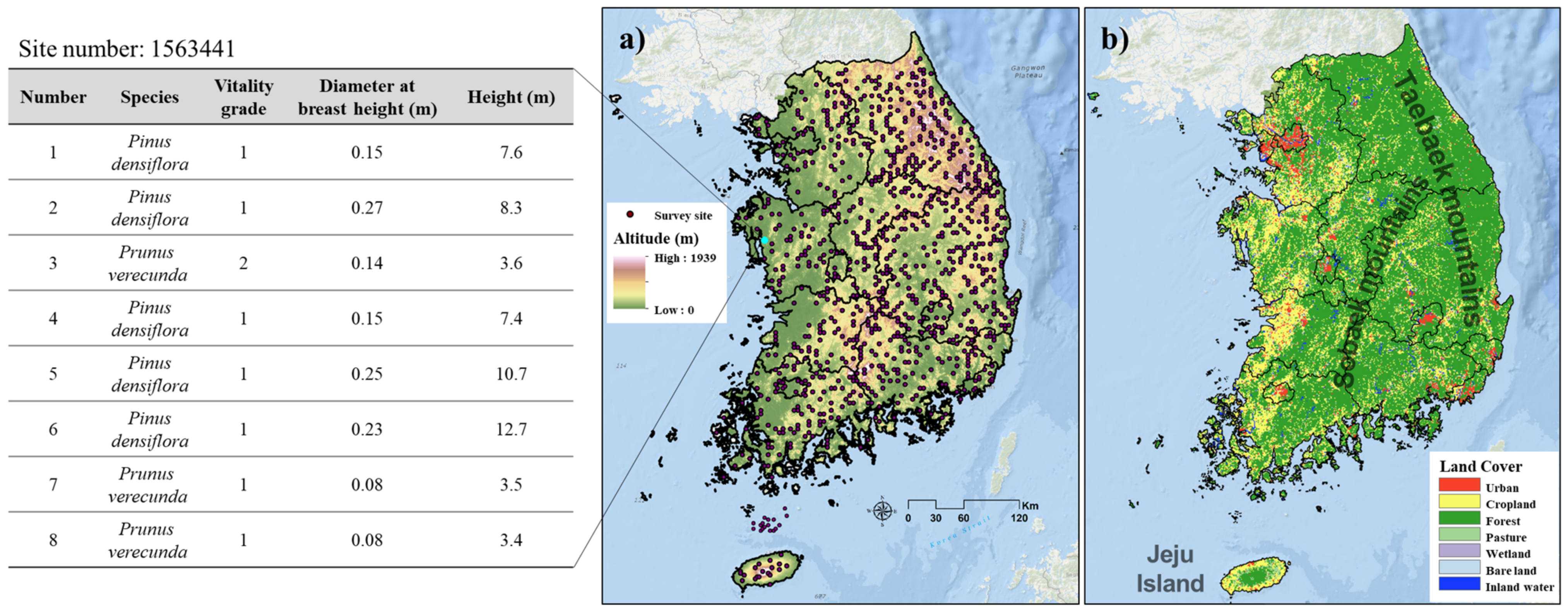
17]. This study used a total of 937 sample plots, excluding sample plots located in non-forest areas, sample plots lacking information on tree species, and sample plots with errors.
The FHM survey examines all trees located within the sample plot, which constitutes 28 indicators in four categories: ‘Tree health’, ‘vegetation health’, ‘soil health’, and ‘atmospheric health’ [
8]. Among various indicators, tree vitality in ‘tree health’ category is recognized as an important indicator to evaluate forest health [
14]. Tree vitality is an index that evaluates the health of a tree based on leaf defoliation, leaf chlorosis, dead branches, or the degree of leaf discoloration [
11,
18]; these indicators are considered to represent the response of trees to overall stress. With weakened tree health, damage occurs in young tissues, such as shoots, branches, and leaves grown in the same year [
18]. Accordingly, forest investigators visually check the condition of leaves and branches of trees in the survey plot to identify tree vitality. Tree vitality is divided into five grades: Healthy, moderately healthy, slightly declined, moderately declined, and severely declined—and specific criteria with indicators are as shown in
Table 1.
In total, there is information on 44,440 trees within 937 sample plots; each sample plot contains from 1 to a maximum of 147 trees (
Figure 1).
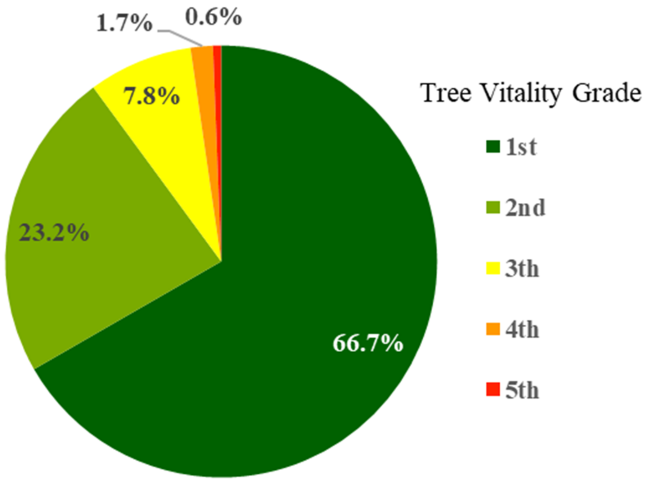
Figure 2 presents the distribution ratio of the surveyed trees by grade, where the 1st and 2nd grades representing healthy trees accounted for ~90% of the total.
3. Materials and Methods
This study utilized tree vitality information to test various methodologies that were designed to construct area-based maps. These vitality data were difficult to spatialize because of the following limitations. Firstly, a representative value was required for each plot for spatialization however, as mentioned in the Introduction, it was difficult to generate representative values using information from multiple individual trees because there is no clear definition of forest health. In particular, as the tree vitality grade is an ordinal variable determined by an expert, it should not be used to represent the health of the stand in the survey plot with a simple average value. The lower the grade, the healthier the tree however, the grading number does not mean that the first grade is twice as healthy as the second grade. In addition, if the mode value within the plot was adopted as a representative value, 67% of plots would be assigned as 1st grade and 25.5% of plots would become 2nd grade; this generates an excessive bias for the 1st and 2nd grades.
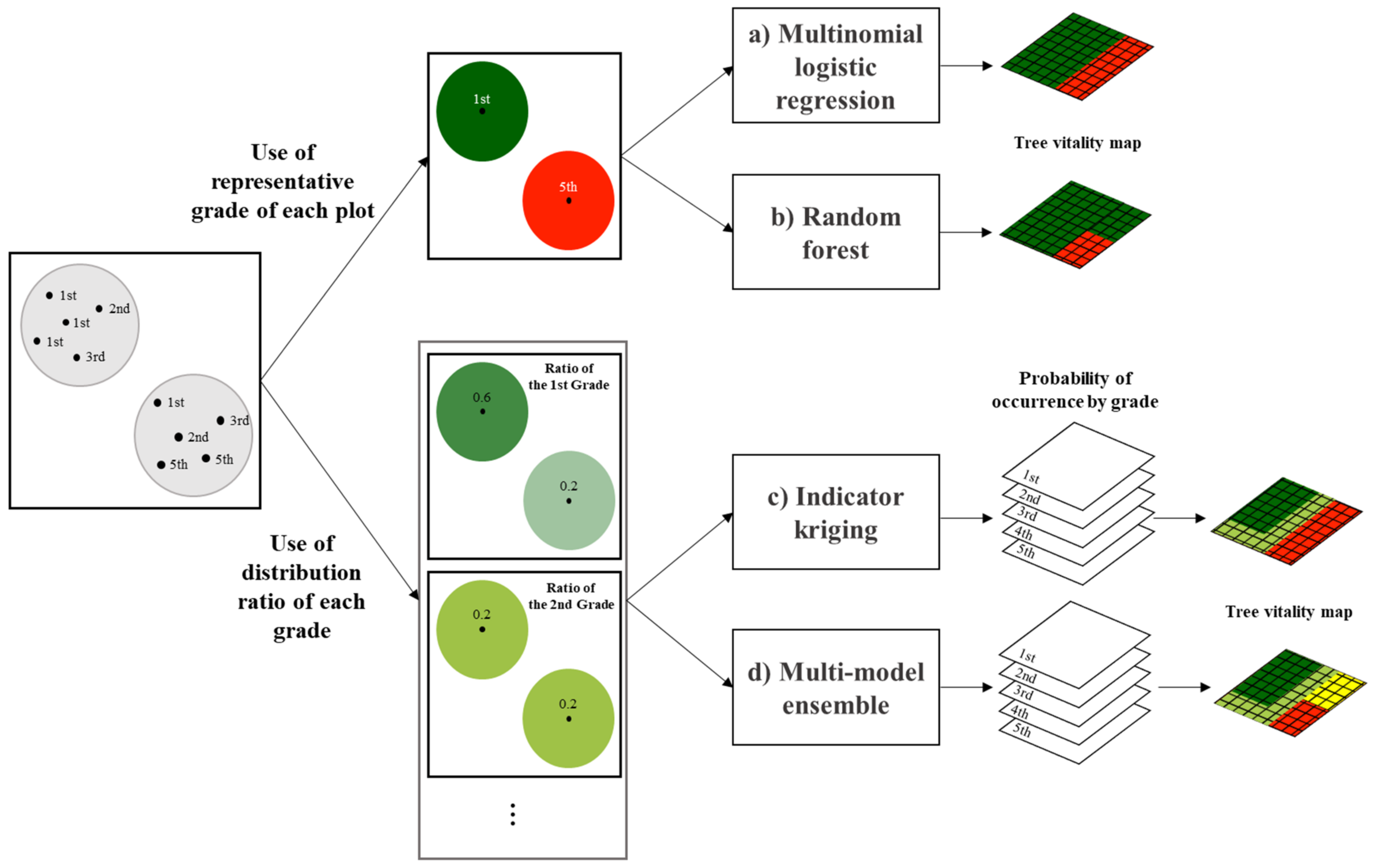
In order to overcome these limitations, we considered the distribution ratio of the grade in the entire survey data to be representative of the true value of the population. As such, a strategy was adopted to allocate the grades by maintaining this ratio, in which two methods were applied (
Figure 3). As this study sought to establish a map to help manage forests, priority was given to unhealthy trees (i.e., in descending order from 5th grade) in both methods.
The first method involved assigning the representative grade in each survey plot based on the overall grade ratio (the true ratio of the population); this was done using the distribution ratio by grade. The 5th grade was assigned to the top 0.6% of plots in the order of the highest 5th grade ratio, the 4th grade was given to the top 1.7% of plots with the highest 4th grade ratio among the remaining survey plots, and the 3rd grade was assigned to the top 7.8% of the remaining plots with the highest 3rd grade ratio. This same method was repeated for the 1st and 2nd grades. After assigning the representative grade for each plot, multinomial logistic regression (MLR) and random forest (RF) classification were utilized to spatialize categorical variables.
The second method involved constructing distribution probability maps for each grade, creating a final grade map by overlapping each probability map. The distribution probability maps for each grade were established using indicator kriging (IK) and a multi-model ensemble (MME) of species distribution models. The latter is a new approach that has been proposed in this study. When overlapping the probability maps, regions were graded in the same way as the first method of assigning representative grades for each plot. That is, the top 0.6% region with a high probability of 5th grade was classified as the 5th grade, and the top 1.7% of the remaining region with a high probability of 4th grade was classified as 4th grade. The same procedure was repeated for the 1st to 3rd grades. A detailed description of each method is provided in
Section 3.1.
3.1. Spatialization Methods
3.1.1. Multinomial Logistic Regression
MLR is considered an important model that may be used to analyze categorical data [
19]. It is an extension of a simple binary logistic regression, predicting the probability of belonging to a category based on multiple independent variables. The regression is generally effective in predicting dependent variables with more than two categories [
20]; independent variables may either be binary or continuous. The maximum likelihood estimation was used to evaluate the probability of belonging to each category.
MLR was run in R software using the nnet-neural network package [
21]. A regression was constructed with all predictors; then, we selected a final model that minimized Akaike information criterion (AIC) through the reduced model.
3.1.2. Random Forest Classification
An RF classification model is an ensemble of tree-type classifiers. Each tree is trained with bootstrapped samples of the original training data using the classification and regression tree (CART) method [
22]. The majority vote of the trees was used to determine the classifier output. Regular decision tree classifiers split nodes based on all feature attributes, whereas the RF algorithm randomly selects a subset of input variables. This random selection scales many features, and reduces interdependence between variable features; this decreases the sensitivity of the algorithm to the inherent noise in the data [
23,
24]. The number of variables to be selected is a user-defined parameter. This study used the default value, the square root of the number of inputs, as the model is insensitive to the number of variables.
The error rate of the RF classifier was dependent on the correlation of any two trees and the classification strength of each individual tree [
24]. The out-of-bag (OOB) error rate indicates the extent to which the forest classifier was successful. The OOB model saves one third of the input dataset to construct the kth tree from the bootstrap sample of each tree. This leftover sample was used to test the misclassification result of the kth tree and the average of all trees [
24]. Although the OOB error estimates do not require cross-validation or a separate test set, validation was conducted using a contingency table to compare models.
3.1.3. Indicator Kriging
IK is a non-parametric type of conditional ordinary kriging that uses local distribution based on location and data values [
25]. It is less sensitive to outlier values, which is useful in analyzing skewed datasets [
26]. This methodology was based on a simple binary transformation where each data point was converted to 0 or 1 using a pre-determined threshold: If values were above the threshold, they were 1, and if they were below the threshold, they were 0. The indicator correlogram was calculated using the transformed dataset, and values of other regions were estimated to be between 0 and 1. This estimate refers to the probability of exceeding the selected critical threshold in these regions.
As the distribution ratio of each grade was used as the input data, the generated results represented the probability of distribution for each grade. The number refers to a probability value exceeding the specified threshold. The IK estimations were conducted using the ArcGIS 10.3.1 software package with Geostatistical Analyst Extensions (ESRI, Redlands, CA, USA).
3.1.4. Multi-Model Ensemble Approach for Tree Vitality Spatialization
We adopted species distribution models (SDMs) to spatialize tree vitality; to the best of our knowledge, this represents the first attempt to do this. SDMs are numerical tools that simulate potential species habitats using records on species occurrence and relevant environmental variables with the associated habitat characteristics [
27]. This type of modeling methodology has long been used to simulate the distribution of species; it has also been applied in a diverse range of applied fields such as medical diagnostics [
28], landslides [
29,
30], and forest fires [
31]. Thus, this study devised a method by which to use SDMs to derive the probabilities of occurrence for each grade.
There are a variety of modeling algorithms to construct SDMs, including regression-based and machine learning-based models; these produce various prediction results for each model. Accordingly, an “ensemble” that combines predictions from these individual models has been promoted as a means to reduce uncertainty and improve accuracy [
32,
33]; as such, an ensemble methodology was applied in this study.
SDMs may be divided into two types based on the required data. The first requires presence data only, and the second requires good-quality presence/absence data [
34,
35,
36]. In most situations, the second type shows better performance [
37]; however, as accurate data on absence are difficult to obtain, many previous studies have only used presence-only data or pseudo-absence data [
37,
38]. This study used data containing good quality presence/absence data, as all tree species within a plot have been thoroughly investigated. The distribution ratio of each grade in the plot was applied as the weight of presence data when establishing the potential distribution map for each grade. The plot in which a specific tree vitality grade does not exist may be used as the absence data. Then, weights for the absence data were assigned as to make the sum of the presence and absence weights equal. Through this method, the absence data for each grade were shown for different weights, resulting in greater absence weights given to the higher grade. This difference in the absence weight for each grade allowed us to overcome the data bias toward the 1st grade.
Seven individual models using presence/absence data were utilized; generalized linear models (GLMs), generalized additive models (GAMs), classification tree analysis (CTA), flexible discriminant analysis (FDA), artificial neural networks (ANN), generalized boosted models (GBM), and RF. We derived the results from each model, and a final map of the potential distribution probability of each grade was established through a weighted average based on the evaluation scores. Finally, a tree vitality grade map was determined by overlapping the potential distribution map of each grade. The BIOMOD2 package was used, as it offers ensemble forecasting software in R [
39].
3.2. Predictor Variables
The presence data used were ordinal variables that divide the degree of tree vitality into five different grades. Thus, it was important to construct predictor variables to be able to explain the different vitalities for each grade. Moreover, as various spatialization models are applied, additional analyses of the tendency and contribution of various predictor variables for each model can be expected. Thus, we collected all available predictor variables that were able to affect tree vitality, limited by data availability.
Vegetation development is highly sensitive to climatic factors, including temperature and precipitation [
40,
41]. Therefore, we collected data on a total of 23 variables reflecting temperature and/or precipitation characteristics, including 19 bioclimatic variables and the warmth index (WI), minimum temperature of the coldest month index (MTCI), precipitation effectiveness index (PEI), and the growing degree days (GDD). Climatic factors were generated using the climatologies at high resolution for the earth’s land surface areas (CHELSA) climate dataset V.1.2. (2004–2013). As the intensity and impact of climate factors vary in terms of different spatial characteristics [
42], three main topographic factors, the digital elevation model (DEM), aspect, and slope, were also considered. Topographic factors were collected from the National Geographic Information Institute database, supported by the Ministry of Land, Infrastructure, and Transport with a 90-m resolution.
The soil factor is a variable that is able to assess tree vitality based on tree growth [
43]. As various soil characteristics impact vegetation structure and vitality [
43,
44], all nine different soil variables available from the World Soil Data (SoilGrids250m 2.0) were collated for the soil factors.
Remote sensing technology is an alternative to conventional methods for monitoring forest health and vitality [
45]. It has been reported that ratio-based indices may successfully detect changes in canopy reflectance, reflecting the decline in tree health status [
46,
47,
48]. Various ratio indices were selected as the final vegetation factors, which include the normalized difference vegetation index (NDVI), atmospherically resistant vegetation index (ARVI), re-normalized difference vegetation index (RDVI), soil adjusted vegetation index (SAVI), and simple ratio (SR) [
45,
49,
50,
51]. These indices were selected by reviewing indices from the Index Data Base (IDB) project operated by the Institute of Crop Science and Resource Conservation (INRES), Germany. Previous studies [
52] have reported that vegetation indices from various periods (from June to September) are used together by combining maximum values. Therefore, this study also uses the maximum value of each vegetation index from June to September, which is the same as the survey period and the summer season in Korea with the highest vegetation vitality. Landsat-5 and Landsat-7 Surface Reflectance Tier 1 images were used to produce the vegetation indices acquired from 2011 to 2015 on Google Earth Engine.
Human-mediated impacts were classified as artificial factors. As urbanization contributes to the degradation of forests [
53], and traffic pollutants threaten vegetation vitality [
54], land cover maps and distances from roads were selected as artificial factors. The data were collected from the Ministry of Environment and Standard Node Links from the National Transport Information Center.
All environmental variables were constructed with available data considering forest survey period (2011–2015) and rescaled at a 1-km
2 resolution. A detailed description of the variables is given in
Supplementary Table S1. They were applied to MLR, RF, and MME, but not to IK.
3.3. Evaluation
The spatialization results of this study were difficult to verify to the same extent as the spatialization itself because of the limitations mentioned in
Section 3; this was mainly because the information on several tree species was contained within one sample plot. Accordingly, we employed a contingency table using the representative values generated for MLR and RF, and generated external independent data that could indirectly indicate tree vitality for pattern-wise verification. In the evaluation, 80% of the data was used as training data, while the remaining 20% was used as test data in the aforementioned models.
3.3.1. Contingency Table (Error Matrix)
Contingency tables for each methodology were developed to compare and analyze the results. The overall accuracy of the classification is computed using these tables; the total number of correct pixels were divided by the total number of pixels in the error matrix. Additionally, we calculated the accuracies of individual grades, including the accuracy of producers and users. The former indicates how well the grades we assigned as representative values of plots were reflected in the final vitality map. The accuracy of users represents the probability that a pixel classified as a specific grade actually represents that grade on the ground. User accuracy is important as our aim is to construct a tree vitality map that may be used for national forest management. In particular, the location of unhealthy forests is a major concern. Therefore, model results were compared focusing on the accuracy of users for 5th grade.
3.3.2. External Validation with Independent Data
The established tree vitality map was qualitatively verified by comparing its distribution patterns with other independent data. As there are few available independent data that spatially indicate tree health, we adopted data that indirectly represents the vitality of vegetation based on literature reviews for validation.
First, the concept of the vegetation condition index (VCI) was adopted; this is an index that expresses the state of vegetation within a specific period by comparing with historical values that represent the best and worst conditions of the vegetation. VCI has been proven to be a good indicator, particularly when assessing the effect of weather on the condition or health of vegetation [
55,
56,
57].
In this study, VCI was constructed using the Moderate Resolution Imaging Spectroradiometer (MODIS) NDVI data from the last 20 years (2001 to 2020). Over this period, each pixel extracted maximum (NDVI
max) and minimum (NDVI
min) NDVI values representing the best and worst vegetation conditions, respectively. To determine the health status of trees in the survey periods, VCI was constructed using the average NDVI (NDVI
avg) for 2011–2015 (Equation (1)):
As MODIS NDVI was produced at 16-d intervals, 460 satellite images were used for 20 years (e.g., two images per month and 23 images per year). We used the MOD13A2 Version 6 product, which provides NDVI at a 1-km spatial resolution, for comparison with a tree vitality map as the same resolution. Image processing was conducted using the Google Earth Engine (
http://earthengine.google.com, accessed on 28 April 2021). For comparative analysis, the VCI was also classified into five grades with the same ratio based on the proportion of the population by grade.
The established maps were also verified using the bioclimate vulnerability index (BVI) suggested by [
58]. The BVI is an index that evaluates the impact of climate change on habitat and spatially presents vulnerable areas. BVI quantified the impact of climate change in terms of moving speed and the area change rate (Equation (2)) of the bioclimatic zone, which are areas with similar environmental characteristics affecting the habitat and species [
58,
59]. The regions with higher BVI are considered as a more vulnerable area to climate change, which can affect the vitality of vegetation [
60]:
Further detailed description for the BVI is provided in Choi et al. (2019). We compared the spatial distribution patterns of bio-climatically vulnerable areas to regions with low tree vitality grades.
4. Results
4.1. Tree Vitality Map
The MLR predictions were dominated by 1st grade (
Figure 4a); almost all pixels (96.46%) were classified as 1st grade, whereby the 2nd, 3rd, and 5th grades accounted for 2.73%, 0.12%, and 0.69%, respectively, and the 4th grade was not given any results. Although the overall accuracy was relatively high (0.68), most regions were classified as 1st grade. Of the remaining grades, only 5th grade was classified at a similar rate to the population. The 2nd, 3rd, and 4th grades could not be mapped to obtain a user accuracy exceeding 6%; this meant that these grades could not be estimated using this methodology and the given set of predictors. Spatially, the distribution of the 5th grade trees was mainly found in the southernmost regions of the Taebaek Mountains and near the summit of Mount Hanlla in the center of Jeju Island. For the 2nd grade, some of the distribution occurred in the midwest plains and northern Jeju Island.
For RF classification, similar to the MLR map, the 1st grade dominated most regions (
Figure 4b), although the percentage occupied was relatively lower at 90.78%. The user accuracy was 0.75 or higher in all grades, with a high overall accuracy of 0.926. The distribution of the 2nd grade was similar to the result of the MLR, although the western coastal regions of Jeju Island were classified as 3rd grade. In the 4th and 5th grades, only pixels in which the plot with those grades were located were classified into these grades; as such, the spatial distribution on the map was almost inconspicuous. This means that the RF overfits with a high accuracy albeit low utilization.
The IK and MME methodologies simulate the distribution probability for each grade and reflect the distribution ratio of the population by using prior-probability at the final map generation; as such, the distribution ratios of grades 1–5 were the same as those of the population. However, as the representative grade for each plot used for verification was not directly trained for those models, they showed a lower accuracy compared to MLR and RF.
IK showed a relatively high user accuracy of 0.642 for the 1st grade and 0.831 for the 2nd grade however, the user accuracy of the 3rd and 4th grades was <0.17. The 5th grade showed almost zero accuracy. From a spatial perspective, 2nd grade was sporadically distributed throughout the country in a clustered form, and 3rd grade was allocated in areas without any spatial characteristics and across Jeju Island. The 4th and 5th grades were also clustered in small areas (
Figure 4c).
The prediction of forest health with MME showed many details corresponding to the existing knowledge of forests. The results of the ensemble model for each grade using the weighted mean probability indicated a high accuracy of a performance value (AUC) over 0.9. However, the overall accuracy, achieved using the contingency table, was only 0.465, due to inconsistent training and validation data. Nevertheless, the user accuracy with the MME result of the 5th grade was 0.8; this was significantly higher than the other models. The 2nd, 3rd, and 4th grades also exhibited accuracies exceeding 0.3, indicating that this MME method was better at predicting lower grades than other models, with the exception of the overfitted RF. The detailed accuracies by grades for each methodology are provided in
Table 2.
The most noticeable result of the MME map is the distribution of the 3rd and 4th grades in alpine regions, a major mountain range in the ROK (
Figure 4d). The 5th grade appeared sporadically in urban neighborhoods and some of the mountainous areas. The southern coastal area and Jeju Island were mainly distributed in 2nd and 3rd grades, while the northern region of Jeju was noticeably distributed in 4th grade. Although the overall accuracy was low, the MME results appeared to have the most plausible results that were likely to be utilized. As such, we further evaluated the MME maps created by comparing distribution patterns with other external independent data in
Section 4.2.
4.2. Validation of the MME Tree Vitality Map
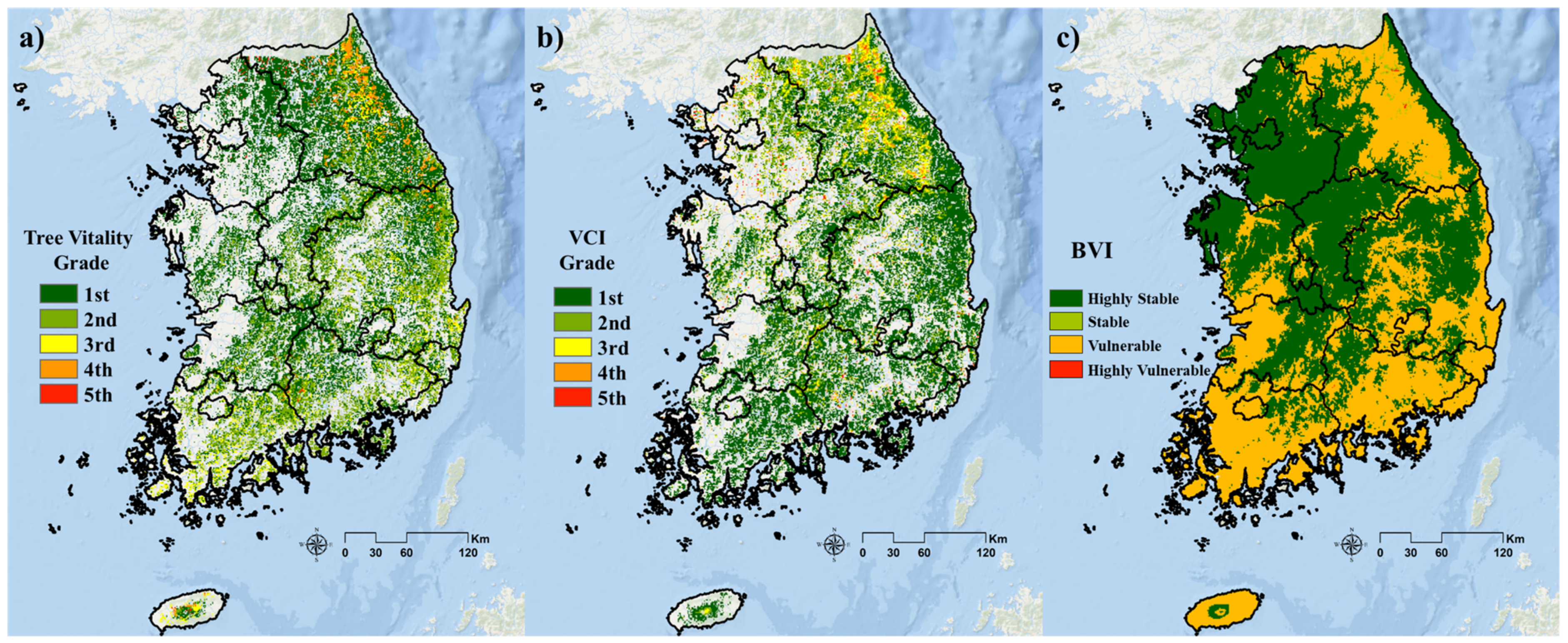
The MME-constructed tree vitality map was compared with the VCI and BVI maps (
Figure 5). All three maps indicate that high-altitude alpine regions are unhealthy or bio-climatically vulnerable. The VCI of forests distributed in the high mountains of Taebak and adjacent areas of urban and agricultural lands were relatively low. Jeju Island has a tendency to lower the VCI with an increasing altitude. The age of trees and the surrounding environments may also be highly influential for tree vitality. This was reflected in the fact that the low grades that appeared in the alpine regions were considered to properly reflect the status of the forest in the ROK; for example, the Taebaek mountains, where very old forests are mainly distributed, are major protected areas. By contrast, the southern region showed a relatively high VCI, which differs from the MME result; this may be because the VCI was created based on NDVI, which is an index highly influenced by tree species, not solely vegetation health.
The BVI represented the degree of vulnerability based on changes in the bioclimate conditions in the 2000s compared to the 1980s; it was found that the most pronounced changes occurred in the southern coastal and alpine regions, including the Taebak Mountains. The similar distribution trends in the low healthy grade region and the bioclimate vulnerable region qualitatively demonstrate the validity of the MME method. Overall, we inferred that climate change is one of the factors that adversely affect the vitality of alpine and southern regions.
5. Discussion
5.1. Summary Comparison of Methods
The attempted MLR and RF classification in this study spatialized representative values for each plot; these were assigned using the distribution ratio of each grade for the population. Although the proportion of grades was the same as the population, almost all regions were classified as 1st grade as a result of MLR; 2nd, 3rd, and 4th grades were unsuitable for prediction. Although the RF was overfit with a very high accuracy, only cells in which the 5th grade sample point was located were classified as this grade. As a result, the spatialization results of both methods were not considered appropriate for use as spatial data for forest management.
For the IK and MME methods, a final grade map was created to reflect the population ratio after spatializing each grade using the proportion by grade within the sample plot. In the resultant maps, the distribution of the five grades was better distinguished than the results of the previous two methodologies. The IK and MME results showed similar spatial tendencies; the former results were more clustered without showing spatial trends, while the latter produced results that properly reflected topographic and climatic characteristics. Comparisons with VCI and BVI demonstrated the usefulness of the MME method. The difference between the IK and MME results may have been a result of IK predicting only the distribution probability based on location and data values, while the MME generated the distribution probability for each grade using environmental predictors that were highly related to tree vitality. Thus, latter produced a more realistic result.
A close comparison of the results of RF and MME showed that the former predicted only pixels containing the 5th grade points as being of the 5th grade and classified most of the surrounding regions as 1st grade however, some MME results classified the areas around the 5th grade points within a diverse range of grades (
Figure 6). This means that the methodologies utilizing the distribution ratio by grade were more suitable than those using plot-specific representative values to reflect the impact of the surrounding environment on predictions of tree vitality.
5.2. Implications and Limitations
Although the survey data of individual trees is meaningful in and of itself, forest management for the country requires area-based forest health assessment as opposed to point data. Therefore, in this study, we explored various methodologies for spatializing grade data from field survey data. A representative value for each plot was required for spatialization therefore, the distribution ratio of the population was utilized in a sample plot or when the final map was being generated. In addition, it presented a method involving the distribution ratio of each grade per sample point. These methodologies can be applied to spatialize other field survey data, such as tree crowns or soil classes. However, to further improve these approaches, the following should be considered.
First, comprehensive indicators are required to evaluate the health of forests, such that all sample points may be represented based on various tree data within the plot and surrounding environment. Although tree vitality was the representative index in this study, it was difficult to evaluate the overall health of the forest using a sample point as a single indicator. The spatialization would have been easier if there were clear criteria for how many or what percentage of declining trees per unit area could be evaluated as an unhealthy forest (i.e., those requiring management). Furthermore, if an indicator could be developed to comprehensively reflect forest health, including crown or soil conditions and tree vitality, it could be used to construct a more robust and reliable national forest health map.
Survey data also needs to be more objectified; as the grade of tree vitality is determined by an expert, it is possible that subjective elements are included depending on the investigator. Therefore, it would be beneficial to develop a methodology that is able to objectively evaluate tree health or investigate tree vitality at an interval or ratio scale while considering spatialization. The convergence of various remote sensing data such as airborne and space-borne datasets with in-situ observations is becoming a means to improve this [
13,
61]. This study attempted an objective evaluation using various satellite-based environmental predictors however, further research on the integration of in-situ and RS monitoring techniques is required to comprehensively assess the status of forest health.
There is also a need to advance environmental predictors. The variables of climate, soil, artificial, and vegetation factors adopted in this study were constructed with different spatial and temporal resolutions. This is because it was difficult to secure high-resolution data on a national scale corresponding to 2011–2015, the same period when the FHM survey was conducted. Accordingly, among the data available to cover the whole country, we used data constructed at the most similar to the forest survey period by resampling them into a 1-km resolution. This temporal and spatial mismatch may raise uncertainty in the results [
62]. Therefore, future studies need to construct and use datasets that match well spatially and temporally with the survey plot in order to create a more accurate forest health map.
Finally, further verification is required to examine whether this methodology can be adopted for managing national forests. In other words, in-situ verification in areas other than sample survey points is required to identify whether forests with a low grade are actually less vital than those assigned to higher grades. It may be useful to produce thematic maps representing national forest health that can represent the actual status of forests and allow their changing trends to be updated continuously.
6. Conclusions
This study examined four methods to construct an area-based map of tree vitality using field survey data as a way of contributing to managing national forests. It also used MRL and RF—methods used to project nominal data—to generate representative values of sample points needed, to evaluate tree vitality grades in regions for which no measurements were available; a new approach was also suggested that used the IK and MME of species distribution models with the distribution ratio of each grade. MRL, RF, and MME employed remotely-sensed environmental datasets. The study showed that RF, in particular, had high accuracy, but underutilized results, while MME proved reasonable based on comparisons with other independent data.
Notably, we found that it is more appropriate to utilize various class information within a sample point for spatialization than using a representative value for each plot. Trees in the alpine or high-altitude regions in the ROK were found to have low vitality, suggesting that the area requires closer investigation and management. This study attempted to enhance the utilization of forest survey data for forest management by integrating various techniques and remotely-sensed environmental predictors.
Author Contributions
Conceptualization, Y.C. and C.-H.L.; Data curation, J.-H.L. and W.I.C.; Investigation, Y.C.; Methodology, Y.C. and H.I.C.; Project administration, W.I.C.; Supervision, S.W.J.; Validation, C.-H.L.; Writing—original draft, Y.C., H.I.C. and J.-H.L.; Writing—review & editing, S.W.J. All authors have read and agreed to the published version of the manuscript.
Funding
This research was funded by the Korea Environmental Industry and Technology Institute (KEITI) through the Decision Support System Development Project for Environmental Impact Assessment (grant number 2020002990009), and the Ministry of Science and ICT through Basic Science Research Projects of the National Research Foundation of Korea (NRF) (grant number 2021R1C1C2012406).
Institutional Review Board Statement
Not applicable.
Informed Consent Statement
Not applicable.
Acknowledgments
The authors gratefully acknowledge the support of the National Institute of Forest Science, the BK21 FOUR program (no. 4120200313708) funded by National Research Foundation of Korea (NRF) and Korea University grant.
Conflicts of Interest
The authors declare no conflict of interest.
References
- Trumbore, S.; Brando, P.; Hartmann, H. Forest health and global change. Science 2015, 349, 814–818. [Google Scholar] [CrossRef] [Green Version]
- FAO. Global Forest Resources Assessment 2020—Key Findings; FAO: Rome, Italy, 2020. [Google Scholar] [CrossRef]
- Choi, Y.; Lim, C.H.; Chung, H.I.; Kim, Y.; Cho, H.J.; Hwang, J.; Kraxner, F.; Biging, G.S.; Lee, W.K.; Chon, J.; et al. Forest management can mitigate negative impacts of climate and land-use change on plant biodiversity: Insights from the Republic of Korea. J. Environ. Manag. 2021, 288. [Google Scholar] [CrossRef]
- Roy, B.A.; Alexander, H.M.; Davidson, J.; Campbell, F.T.; Burdon, J.J.; Sniezko, R.; Brasier, C. Increasing forest loss worldwide from invasive pests requires new trade regulations. Front. Ecol. Environ. 2014, 12, 457–465. [Google Scholar] [CrossRef] [Green Version]
- Lim, C.H.; Yoo, S.; Choi, Y.; Jeon, S.W.; Son, Y.; Lee, W.K. Assessing climate change impact on forest habitat suitability and diversity in the Korean Peninsula. Forests 2018, 9, 259. [Google Scholar] [CrossRef] [Green Version]
- Potter, K.M.; Conkling, B.L. Forest Health Monitoring: National Status, Trends, and Analysis 2014; General Technical Report-Southern Research Station; Southern Research Station, USDA Forest Service: Asheville, NC, USA, 2015; (SRS-209).
- Yang, J.; Dai, G.; Wang, S. China’s national monitoring program on ecological functions of forests: An analysis of the protocol and initial results. Forests 2015, 6, 809–826. [Google Scholar] [CrossRef]
- Park, B.B.; Han, S.H.; Rahman, A.; Choi, B.A.; Im, Y.S.; Bang, H.S.; So, S.J.; Koo, K.M.; Park, D.Y.; Kim, S.B.; et al. Brief history of Korean national forest inventory and academic usage. Korean J. Agric. Sci. 2016, 43, 299–319. [Google Scholar] [CrossRef] [Green Version]
- Wingfield, M.J.; Brockerhoff, E.G.; Wingfield, B.D.; Slippers, B. Planted forest health: The need for a global strategy. Science 2015, 349, 832–836. [Google Scholar] [CrossRef] [PubMed]
- McDowell, N.G.; Coops, N.C.; Beck, P.S.A.; Chambers, J.Q.; Gangodagamage, C.; Hicke, J.A.; Huang, C.; Kennedy, R.; Krofcheck, D.J.; Litvak, M.; et al. Global satellite monitoring of climate-induced vegetation disturbances. Trends Plant. Sci. 2015, 20, 114–123. [Google Scholar] [CrossRef] [Green Version]
- Lausch, A.; Erasmi, S.; King, D.J.; Magdon, P.; Heurich, M. Understanding forest health with remote sensing-part I—A review of spectral traits, processes and remote-sensing characteristics. Remote Sens. 2016, 8, 1029. [Google Scholar] [CrossRef] [Green Version]
- Lausch, A.; Erasmi, S.; King, D.J.; Magdon, P.; Heurich, M. Understanding forest health with remote sensing-part II—A review of approaches and data models. Remote Sens. 2017, 9, 129. [Google Scholar] [CrossRef] [Green Version]
- Pause, M.; Schweitzer, C.; Rosenthal, M.; Keuck, V.; Bumberger, J.; Dietrich, P.; Heurich, M.; Jung, A.; Lausch, A. In situ/remote sensing integration to assess forest health—A review. Remote Sens. 2016, 8, 471. [Google Scholar] [CrossRef] [Green Version]
- Cherubini, P.; Battipaglia, G.; Innes, J.L. Tree Vitality and Forest Health: Can Tree-Ring Stable Isotopes Be Used as Indicators? Curr. For. Rep. 2021, 7, 69–80. [Google Scholar]
- Kolb, T.; Wagner, M.; Covington, W.W. Concepts of forest health: Utilitarian and ecosystem perspectives. J. For. 1994, 92. [Google Scholar] [CrossRef]
- Ferretti, M. Forest health assessment and monitoring–issues for consideration. Environ. Monit. Assess. 1997, 48, 45–72. [Google Scholar] [CrossRef]
- Lee, J.H.; Ryu, J.E.; Choi, Y.Y.; Chung, H.I.; Jeon, S.W.; Lim, J.H.; Choi, H.S. Spatial Estimation of Forest Species Diversity Index by Applying Spatial Interpolation Method-Based on 1st Forest Health Management data. J. Korean Soc. Environ. Restor. Technol. 2019, 22, 1–14. [Google Scholar]
- Kim, S.H.; Sung, J.H.; Koo, N.I.; Kim, Y.S.; Kim, K.H. The 1st Forest Health and Vitality Diagnosis and Evaluation Report; National Institute of Forest Science: Seoul, Korea, 2016; ISBN 9788981761257.
- El-Habil, A.M. An application on multinomial logistic regression model. Pak. J. Stat. Oper. Res. 2012, 8, 271–291. [Google Scholar] [CrossRef]
- Starkweather, J.; Moske, A.K. Multinomial Logistic Regression. 2011. Available online: http://www.unt.edu/rss/class/Jon/Benchmarks/MLR_JDS_Aug2011.pdf (accessed on 3 June 2021).
- Ripley, B.; Venables, W.; Ripley, M.B. Package ‘nnet’. R Package Version; R Foundation for Statistical Computing: Vienna, Austria, 2016. [Google Scholar]
- Palczewska, A.; Palczewski, J.; Robinson, R.M.; Neagu, D. Interpreting random forest classification models using a feature contribution method. In Integration of Reusable Systems; Springer: Cham, Switzerland, 2014; pp. 193–218. [Google Scholar]
- Criminisi, A.; Shotton, J.; Konukoglu, E. Decision forests: A unified framework for classification, regression, density estimation, manifold learning and semi-supervised learning. Found. Trends® Comput. Graph. Vis. 2012, 7, 81–227. [Google Scholar] [CrossRef]
- Alam, M.S.; Vuong, S.T. Random forest classification for detecting android malware. In Proceedings of the 2013 IEEE International Conference on Green Computing and Communications and IEEE Internet of Things and IEEE Cyber, Physical and Social Computing, Washington, DC, USA, 20−23 August 2013; pp. 663–669. [Google Scholar]
- Hohn, M. Geostatistics and Petroleum Geology, 2nd ed.; Springer Science & Business Media: Berlin/Heidelberg, Germany, 1999; pp. 151–155. ISBN 978-94-011-4425-4. [Google Scholar]
- Smith, J.L.; Halvorson, J.J.; Papendick, R.I. Using multiple-variable indicator kriging for evaluating soil quality. Soil Sci. Soc. Am. J. 1993, 57, 743–749. [Google Scholar] [CrossRef]
- Guisan, A.; Tingley, R.; Baumgartner, J.B.; Naujokaitis-Lewis, I.; Sutcliffe, P.R.; Tulloch, A.I.; Regan, T.J.; Brotons, L.; McDonald-Madden, E.; Mantyka-Pringle, C.; et al. Predicting species distributions for conservation decisions. Ecol. Lett. 2013, 16, 1424–1435. [Google Scholar] [CrossRef]
- Hand, D.J. Statistical methods in diagnosis. Statist. Methods Med. Res. 1992, 1, 49–67. [Google Scholar] [CrossRef]
- Kim, H.; Lee, D.K.; Mo, Y.; Kil, S.; Park, C.; Lee, S. Prediction of landslides occurrence probability under climate change using MaxEnt model. J. Environ. Impact Assess. 2013, 22, 39–50. [Google Scholar] [CrossRef] [Green Version]
- Park, N.W. Using maximum entropy modeling for landslide susceptibility mapping with multiple geoenvironmental data sets. Environ. Earth Sci. 2015, 73, 937–949. [Google Scholar] [CrossRef]
- Lim, C.H.; Kim, Y.S.; Won, M.; Kim, S.J.; Lee, W.K. Can satellite-based data substitute for surveyed data to predict the spatial probability of forest fire? A geostatistical approach to forest fire in the Republic of Korea. Geomat. Nat. Hazards Risk 2019, 10, 719–739. [Google Scholar] [CrossRef] [Green Version]
- Araújo, M.B.; New, M. Ensemble forecasting of species distributions. Trends Ecol. Evol. 2007, 22, 42–47. [Google Scholar] [CrossRef]
- Grenouillet, G.; Buisson, L.; Casajus, N.; Lek, S. Ensemble modelling of species distribution: The effects of geographical and environmental ranges. Ecography 2011, 34, 9–17. [Google Scholar] [CrossRef]
- Hirzel, A.; Guisan, A. Which is the optimal sampling strategy for habitat suitability modelling. Ecol. Model. 2002, 157, 331–341. [Google Scholar] [CrossRef]
- Pearce, J.L.; Boyce, M.S. Modelling distribution and abundance with presence-only data. J. Appl. Ecol. 2006, 43, 405–412. [Google Scholar] [CrossRef]
- Aarts, G.; Fieberg, J.; Matthiopoulos, J. Comparative interpretation of count, presence–absence and point methods for species distribution models. Methods Ecol. Evol. 2012, 3, 177–187. [Google Scholar] [CrossRef]
- Brotons, L.; Thuiller, W.; Araújo, M.B.; Hirzel, A.H. Presence-absence versus presence-only modelling methods for predicting bird habitat suitability. Ecography 2004, 27, 437–448. [Google Scholar] [CrossRef] [Green Version]
- Barbet-Massin, M.; Jiguet, F.; Albert, C.H.; Thuiller, W. Selecting pseudo-absences for species distribution models: How, where and how many? Methods Ecol. Evol. 2012, 3, 327–338. [Google Scholar] [CrossRef]
- Thuiller, W.; Lafourcade, B.; Engler, R.; Araújo, M.B. BIOMOD—A platform for ensemble forecasting of species distributions. Ecography 2009, 32, 369–373. [Google Scholar] [CrossRef]
- Dulamsuren, C.; Hauck, M.; Khishigjargal, M.; Leuschner, H.H.; Leuschner, C. Diverging climate trends in Mongolian taiga forests influence growth and regeneration of Larix sibirica. Oecologia 2010, 163, 1091–1102. [Google Scholar] [CrossRef] [Green Version]
- Gunin, P.D.; Vastokova, E.A.; Dorofeyuj, N.I.; Tarasov, P.E.; Black, C.C. Vegetation Dynamics of Mongolia; Springer Science & Business Media: Berlin/Heidelberg, Germany, 1999; ISBN 978-94-015-9143-0. [Google Scholar]
- Klinge, M.; Dulamsuren, C.; Erasmi, S.; Karger, D.N.; Hauck, M. Climate effects on vegetation vitality at the treeline of boreal forests of Mongolia. Biogeosciences 2018, 15, 1319–1333. [Google Scholar] [CrossRef] [Green Version]
- Kim, S.K.; Park, S.B.; Nam, J.C.; Kim, S.H. Effects of location and soil characteristics on the vegetation structure and tree vitality of urban park and green open space. J. Korean Soc. Environ. Restor. Technol. 2002, 5, 30–44. [Google Scholar]
- Kim, E.Y.; Jung, K.M. Analysis of health status of street trees and major affecting factors on Deogyeong-daero in Suwon. J. Korean Soc. Environ. Restor. Technol. 2019, 22, 49–57. [Google Scholar]
- Ismail, R.; Mutanga, O.; Bob, U. Forest health and vitality: The detection and monitoring of Pinus patula trees infected by Sirex noctilio using digital multispectral imagery. S. Hemisph. For. J. 2007, 69, 39–47. [Google Scholar] [CrossRef]
- Ekstrand, S. Assessment of forest damage with Landsat TM: Correction for varying forest stand characteristics. Remote Sens. Environ. 1994, 47, 291–302. [Google Scholar] [CrossRef]
- Nelson, R.F. Detecting forest canopy change due to insect activity using Landsat MSS. Photogramm. Eng. Remote Sens. 1983, 49, 1303–1314. [Google Scholar]
- Vogelmann, J.E. Comparison between two vegetation indices for measuring different types of forest damage in the north-eastern United States. Int. J. Remote Sens. 1990, 11, 2281–2297. [Google Scholar] [CrossRef]
- Hong, W.Y.; Park, M.J.; Park, J.Y.; Park, G.A.; Kim, S.J. The spatial and temporal correlation analysis between MODIS NDVI and SWAT predicted soil moisture during forest NDVI increasing and decreasing periods. KSCE J. Civ. Eng. 2010, 14, 931–939. [Google Scholar] [CrossRef]
- Cho, S.H.; Lee, G.S.; Hwang, J.W. Drone-based vegetation index analysis considering vegetation vitality. J. Korean Assoc. Geogr. Inf. Stud. 2020, 23, 21–35. [Google Scholar]
- Erdenesumbee, S.; Lee, G.S.; Choi, Y.W.; Song, J.K.; Cho, G.S. The Desertification Analysis of Mongolia using Grain Size Index and Vegetation Cover Index. Korean Assoc. Cadastre Inform. 2017, 19, 73–86. [Google Scholar] [CrossRef]
- Albarakat, R.; Lakshmi, V. Comparison of Normalized Difference Vegetation Index derived from Landsat, MODIS, and AVHRR for the Mesopotamian marshes between 2002 and 2018. Remote Sens. 2019, 11, 1245. [Google Scholar] [CrossRef] [Green Version]
- Sejati, A.; Buchori, I.; Rudiarto, I. The impact of urbanization to forest degradation in Metropolitan Semarang: A preliminary study. In IOP Conference Series: Earth and Environmental Science; IOP Publishing: Bristol, UK, 2018; p. 012011. [Google Scholar]
- Gadsdon, S.R.; Power, S.A. Quantifying local traffic contributions to NO2 and NH3 concentrations in natural habitats. Environ. Pollut. 2009, 157, 2845–2852. [Google Scholar] [CrossRef]
- Gitelson, A.A.; Kogan, F.; Zakarin, E.; Spivak, L.; Lebed, L. Using AVHRR data for quantitative estimation of vegetation conditions: Calibration and validation. Adv. Space Res. 1998, 22, 673–676. [Google Scholar] [CrossRef]
- Park, J.S.; Kim, K.T.; Choi, Y.S. Application of vegetation condition index and standardized vegetation index for assessment of spring drought in South Korea. In Proceedings of the IGARSS 2008—2008 IEEE International Geoscience and Remote Sensing Symposium, Boston, MA, USA, 7–11 July 2008; Volume 3, p. III-774. [Google Scholar]
- Dutta, D.; Kundu, A.; Patel, N.R.; Saha, S.K.; Siddiqui, A.R. Assessment of agricultural drought in Rajasthan (India) using remote sensing derived Vegetation Condition Index (VCI) and Standardized Precipitation Index (SPI). Egypt. J. Remote Sens. Space Sci. 2015, 18, 53–63. [Google Scholar] [CrossRef] [Green Version]
- Choi, Y.; Lim, C.-H.; Chung, H.I.; Ryu, J.; Jeon, S.W. Novel Index for bioclimatic zone-based biodiversity conservation strategies under climate change in Northeast Asia. Environ. Res. Lett. 2019, 14, 124048. [Google Scholar] [CrossRef]
- Choi, Y.; Lim, C.H.; Ryu, J.; Jeon, S.W. Bioclimatic classification of Northeast Asia reflecting social factors: Development and characterization. Sustainability 2017, 9, 1137. [Google Scholar] [CrossRef] [Green Version]
- Sicard, P.; Dalstein-Richier, L. Health and vitality assessment of two common pine species in the context of climate change in southern Europe. Environ. Res. 2015, 137, 235–245. [Google Scholar] [CrossRef]
- Lawley, V.; Lewis, M.; Clarke, K.; Ostendorf, B. Site-based and remote sensing methods for monitoring indicators of vegetation condition: An Australian review. Ecol. Indic. 2016, 60, 1273–1283. [Google Scholar] [CrossRef] [Green Version]
- Pacifici, K.; Reich, B.J.; Miller, D.A.; Pease, B.S. Resolving misaligned spatial data with integrated species distribution models. Ecology 2019, 100, e02709. [Google Scholar] [CrossRef] [PubMed]
| Publisher’s Note: MDPI stays neutral with regard to jurisdictional claims in published maps and institutional affiliations. |
© 2021 by the authors. Licensee MDPI, Basel, Switzerland. This article is an open access article distributed under the terms and conditions of the Creative Commons Attribution (CC BY) license (https://creativecommons.org/licenses/by/4.0/).


 ,
, 


