Stable Coexistence in a Field-Calibrated Individual-Based Model of Mangrove Forest Dynamics Caused by Inter-Specific Crown Plasticity

Abstract

(1,2) In this theoretical study, we apply MesoFON, a field-calibrated individual-based model of mangrove forest dynamics, and its Lotka–Volterra interpretations to address two questions: (a) Do the dynamics of two identical red mangrove species that compete for light resources and avoid inter-specific competition by lateral crown displacement follow the predictions of classical competition theory or resource competition theory? (b) Which mechanisms drive the dynamics in the presence of inter-specific crown plasticity when local competition is combined with global or with localized seed dispersal? (3) In qualitative support of classical competition theory, the two species can stably coexist within MesoFON. However, the total standing stock at equilibrium matched the carrying capacity of the single species. Therefore, a “non-overyielding” Lotka–Volterra model rather than the classic one approximated best the observed behavior. Mechanistically, inter-specific crown plasticity moved heterospecific trees apart and pushed conspecifics together. Despite local competition, the community exhibited mean-field dynamics with global dispersal. In comparison, localized dispersal slowed down the dynamics by diminishing the strength of intra-/inter-specific competition and their difference due to a restriction in the competitive race to the mean-field that prevails between conspecific clusters. (4) As the outcome in field-calibrated IBMs is mediated by the competition for resources, we conclude that classical competition mechanisms can override those of resource competition, and more species are likely to successfully coexist within communities.

1. Introduction

Individual-based models (IBMs) simulate the complex life-cycle of individual organisms, including their usage of dynamic resources and their variation among each other within and between life-stages [1]. Frequently, the dynamics of field-calibrated individual-based models of plant communities have deviated from the behavior of a mean field [2], where “individual organisms encounter one another in proportion to their average abundance across space” [3] or, more stringently formulated, “where the interactions are global, that is mortality depends on global density and/or dispersal is infinite” [4]. This has been demonstrated by comparing the dynamics of two models: the original IBM in which interactions among plants and/or the dispersal of seeds were local (in line with natural conditions) and a model in which interactions/dispersal were artificially extended and made global. Pacala and Deutschman (1995) [5], for instance, developed a mean-field model in which the horizontal spatial heterogeneity inherent in the individual-based forest growth model SORTIE was removed and only the vertical heterogeneity among trees was retained. Due to an absence of gaps, their mean-field model maintained only approximately half of the standing crop and it lost diversity in the succession about twice as fast as the full spatial model [5]. In general terms, spatial patterns assumed to indiscriminately arise in the IBMs from local competition and localized seed dispersal have been made responsible for the deviations [2].

This has led to the belief that real plant communities cannot be simulated by mean-field models and that IBMs are necessary to accomplish this task. On the other hand, the persistence of this belief has prevented the contribution of individual-based modeling to the ultimate question of plant ecology: Why do so many plant species coexist in plant communities?

1.1. Theories of Plant Competition

For more than 90 years, coexistence and biodiversity theorists have sought to address this question largely by way of mean-field models. In Appendix A, we give an overview of the opposing theories on the coexistence of competing species: (1) the classical competition theory founded on the Lotka–Volterra (LV) model [6,7], (2) the resource competition theory, including (2.1) the resource ratio hypothesis [8] and (2.2) the resource co-limitation theory. Recently, mounting evidence of nitrogen/phosphorus co-limitation (N/P co-limitation), thus supporting theory 2.2, has been found in terrestrial, freshwater, and marine ecosystems from meta-analyses of large numbers of fertilization experiments [9,10].

Within this study, we point out the major difference among the two main theories in terms of the competition for a single resource: In the classical theory, stable coexistence at an over-yielding equilibrium—one that exceeds the carrying capacities of the single species—is enabled when intra-specific competition is stronger than inter-specific competition. The coexistence is defined here by biotic interactions alone and is, thus, valid for any number of resources. In resource competition theory, two species deplete a common resource until a resource level R* is finally reached, at which only the best competitive species can survive [8]. Hence, in the competition for one resource, coexistence no longer exists. There is, in fact, only one best competitor. We assume here that resource co-limitation theory (2.2) condenses to the R* theory (2.1) in the single resource case (compare [11]).

1.2. Recent Developments of Individual-Based Modeling

The work of Adams et al. (2011) [12] has cast doubts on the belief that IBMs and mean-field models are distinct: In their study on Scots Pine, the effect of space (local interaction) on tree density and basal area was minor, the trajectories of density for the mean-field and spatial models were almost indiscernible, and the basal area at equilibrium was only 10% lower in the mean-field model. The authors stated that such small discrepancies between spatial IBMs and mean-field models are commonly observed in temperate forests (Deutschman et al., 1999; Busing and Mailly, 2004, cited in [12]). Larger discrepancies only developed when either the tree density or the neighborhood size was artificially lowered or when the interaction strength was unnaturally raised. After all, the work of Adams et al. [12] opens the way to a contribution of the IBM to the competition theory.

Localized seed dispersal is the second important process that might induce deviations from mean-field behavior in IBMs, because it leads to conspecific clustering [13]. The results of Adams et al. [12] were less clear in this regard. Local dispersal is generally considered an equalizing coexistence mechanism [14,15,16,17] that, by definition, slows the community dynamics but does not alter the competitive outcome among the species. However, not much is known about the mechanisms by which local dispersal prompts this slowing of dynamics.

During the past two decades, individual-based modelers, in particular, the developers of the SORTIE model, have made considerable efforts to replace the old approximation of a tree crown as a rigid cylinder by a new approximation in which a crown is able to change its shape flexibly (cylinder, ellipsoid, and cone) and move laterally [18]. While the most critical biological shortcoming of the SORTIE model could be overcome [19], the modification brought about another dilemma. SORTIE, already complicated prior to the modification, turned into a mathematically intractable model. As a solution, the authors translated all spatial stochastic processes of SORTIE to a macroscopic partial differential equation, the von Foerster equation, using a perfect plasticity approximation (PPA) [18].

Intrigued by the work of Strigul et al., Grueters et al. (2014) [20] aimed to gain insight into the role crown plasticity could play in mangrove ecosystems. The authors developed MesoFON, a new individual-based and field-calibrated model of mangrove forest dynamics that advances beyond current models by describing the crown plasticity of mangrove trees. They applied a simpler approach to crown plasticity than the SORTIE developers. Their routines took advantage of the Fields-Of-Neighborhood (FON) approach, a general-purpose, position-dependent competition index ([21], see [22] for the concepts of competition indices), and they accounted for the trunk bending and the differential side branch growth mechanism as Strigul et al. did [18], but, in contrast to those researchers, they ignored the flexibility of the crown shape, because this is not as important in mangroves as in temperate forests, which may consist of coniferous species possessing conical crowns and deciduous species owning ellipsoidal crowns.

More recently, efforts have been made to integrate MesoFON into an ecosystem model to be able to simulate the impact of large-scale threats, such as eutrophication and altered sedimentation/hydrology [23], on the wide range of valuable ecosystem goods and services provided by mangroves (compare [24], Appendix A in particular).

As all field-calibrated IBMs, MesoFON is implicitly resource-based. “Implicitly resource-based” here means that the resource (co-)limitation is accounted for in the IBM via mathematical functions, but the uptake of mineral resources from the soil into plants and their return to the soil by the decay of litter is not simulated explicitly mechanistically therein. The competition for above- and below-ground resources is dealt with separately in the MesoFON model assuming resource co-limitation. In the first application of the model, Grueters et al. [20] exposed two plant functional types of the red mangrove (Rhizophora mangle L.), one with plastic and the other with rigid crowns, to two disturbance regimes, namely (1) without disturbance and (2) with hurricane impacts returning every 5 years. The major finding of this simulation study was that disturbances strongly promoted the beneficial effects of crown plasticity. Without disturbances, the overall high competitive strength constrained the effects of plasticity in the dense stands, whereas in the treatment with hurricane impacts, crown shifts were particularly advantageous because of their contribution to gap closure.

1.3. Objectives of This Study

By contrast, in this study, we aimed to discern which of the above theories explains the competitive dynamics in the MesoFON IBM. We adopted an explorative case study approach [25,26,27] and designed a critical case [25] toward this end.

The chosen case consists of two equivalent species that are identical in all respects and inherit their entire behavior from Rhizophora mangle. Resource competition theory predicts that a community of two equivalent (or identical) species is only neutrally stable [28] and that it either fluctuates forever [28] or one of the species goes extinct in a random walk (own judgement). Given that MesoFON is implicitly resource-based, we expect competitive dynamics in MesoFON to follow this prediction. As detailed in the Materials and Methods (Section 2.1), the growth, competition, and dispersal attributes of Rhizophora mangle make this a typical case of a pioneer tree species with a fast initial, but later average, growth, short-distance competitive interaction (due to the medium size of mature trees), and moderate dispersal distance, while we ignore the long tail of the species’ dispersal kernel in this study (compare Section 2.1.1). It is emphasized that the growth parameters under the optimal environmental conditions applied here are not affected by the physiological, morphological, and ecological adaptations (salt tolerance, aerial roots, vivipary, and hydrochory) that allow the red mangrove to survive in intertidal tropical regions.

Furthermore, we compare community dynamics when local competition is applied alone (with global dispersal) or when it is combined with localized seed dispersal. We aim to verify that IBM dynamics solely with local competitive interactions, as observed in the field, are in accordance with the conclusions of Adams et al. (2011) [12] and resemble those of a mean-field. We expect that the combination of localized dispersal combined with local interaction would slow competitive dynamics and lead to some form of conspecific clustering. If so, we pay special attention to examine the mechanisms by which this behavior occurs.

In the end, we transform the case study into a critical one by injecting inter-specific crown plasticity, as we call it, into the scene. Toward this end, we establish exclusively a (hard-coded) avoidance of inter-specific neighbors by lateral crown displacement in MesoFON. This should raise intra-specific competition over inter-specific competition. If classical competition theory holds, the two equivalent (or identical) species should coexist at a stable equilibrium [6,7], whereas the community of equivalent species should only be neutrally stable if resource competition theory holds ([28], see above). The setup of the cases study is graphically illustrated as part of the workflow diagram in Appendix B, Figure A1.

The typical case is already simplistic, even minimalistic, serving to prevent the potential danger of misidentifying mechanisms. Of course, the critical case was ultimately artificial. Even though the transformation into the critical case was justified by scientific evidence from field surveys that crown plasticity is stronger in mixed than in pure stands [29], the artificiality of the critical case requires us to evaluate the implications of our results for field surveys. We provide such a resolution in the final discussion section.

2. Materials and Methods

2.1. MesoFON—An Individual-Based Model of Mangrove Forest Dynamics

The MesoFON model simulates mangrove forest dynamics as they emerge from the recruitment, establishment, growth, and death of individual mangrove trees, and their spatially explicit above-/below-ground interaction.

In light of the objectives and the community under study, we chose to start each simulation with an empty plot of two hectares. Patch sizes of two hectares and beyond are common among Rhizophora mangle forests, in the Southwest of Florida, for instance [30]. Initially, a number of saplings was randomly placed on the plot, thereby mimicking a severe disturbance event at the beginning. We let the community pass through an initial re-colonization phase until it achieved a steady-state (after 500 annual time intervals, set to 1000 years to be on the safe side), and we maintained it in the steady-state for a further 7000 simulation years. This procedure allowed us to compare the state in which most mangrove communities reside, namely the re-colonization, with the state primarily considered in theoretical models, i.e., the steady-state.

The state of an individual tree is specified in mesoFON by its age, diameter at 1.37 m height (d_1.37), diameter growth during the preceding 5 years, x,y-position of its stem base, and the possibly shifted x,y-position of its crown center. An important new state variable is the intra-/inter-specific competition that a tree experiences from its neighbors. Other variables, such as tree height, basal area, and stem volume, are derived from the state variables.

The following series of processes was scheduled for individual trees, to be executed at the conclusion of each annual time interval: (1) tree recruitment, including propagule production, and random global or natural propagule dispersal by water localized around the parental trees, (2) tree growth, (3) growth reduction due to above-ground competition and below-ground competition, (4) lateral crown displacement, and (5) tree death. The processes were implemented as follows:

2.1.1. Tree Recruitment

Recruitment includes propagule production and random global or natural localized propagule dispersal. Under optimal conditions, the density of propagules D (m⁻³) per crown surface area A (m³) is assumed to remain constant during the lifetime of a tree, so the propagule production rate increases with the size of the tree. The density parameter D is set to resemble sapling numbers established per hectare per year, as measured by Chen and Twilley (1998) [31]. Overall, seed production scales less with tree size using MesoFON, relative to other models [20]. Due to competition, propagule production deviates downward, compared with this optimal behavior.

Irrespective of the dispersal regime (global or localized), the placement of saplings is the sole stochastic process in the model. The localized propagule dispersal by water around parental trees represents the single extension to the previous model [20]; thus, details of corresponding dispersal routines are described in the following discussion. We assume that flowers are primarily produced by terminal branches. Thus, propagules are released exclusively from random x,y-coordinates on the crown margins. After landing on the water surface at the x,y-position of release, a propagule is transported forward by water in steps of 1 m in the direction of the water current that is randomly chosen from 0° to 360° for each propagule. The specific behavior is defined by Equation (1):

$$\mathrm{P}\mathrm{o}\mathrm{s}{\left(\mathrm{x},\mathrm{y}\right)}_{\mathrm{n}+1}=\left\{\begin{array}{c}\mathrm{i}\mathrm{f} \mathrm{x}\le {\mathrm{P}}_{\mathrm{s}\mathrm{p}\mathrm{r}\mathrm{e}\mathrm{a}\mathrm{d}}\to \mathrm{P}\mathrm{o}\mathrm{s}{\left(\mathrm{x},\mathrm{y}\right)}_{\mathrm{n}}+\overrightarrow{\mathrm{u}}\\ \mathrm{i}\mathrm{f} \mathrm{x}>{\mathrm{P}}_{\mathrm{s}\mathrm{p}\mathrm{r}\mathrm{e}\mathrm{a}\mathrm{d}}\to \mathrm{P}\mathrm{o}\mathrm{s}{\left(\mathrm{x},\mathrm{y}\right)}_{\mathrm{n}} \end{array}\right.$$

(1)

where Pos(x,y)_n+1 is the x,y-position of a propagule at step n+1, x is a random number taken from a uniform distribution defined over the closed interval [0,1], P_spread = 0.9 represents the spread probability, and $\overrightarrow{\mathrm{u}}$ is a unit vector pointing in the direction of the water current.

The dispersal pattern established by this routine mimicks a negative exponential kernel [32]. In order to reduce the number of simulated individuals, trees are established as saplings rather than as seedlings in the model.

With the parameters defined above, the simulation creates a simple geometric distribution of propagule distances, all defined relative to a starting point at the crown margin of a parental tree. The mean and maximum dispersal distances of 100 propagules were computed as 9.09 and 39.91 m, respectively.

In the following, we aimed to assess the realism of the simulated dispersal kernel for Rhizophora mangle and its representativeness for larger parts of the tree flora. In principle, the simulated dispersal distances are in good qualitative agreement with recent findings on the Rhizophora genus. The majority of Rhizophora mucronata Lamk. propagules remained in a 20 m vicinity of the parental tree, and only few were carried more than 65 m away (Chan and Hursin 1985, cited in [30]). In release experiments carried out by Van der Stocken et al. [33], more than 50% of the R. mucuronata propagules were recovered at distances less than 20 m, and only 1% were recovered at distances of more than 90 m. In a further study, Sousa et al. [34] recovered all painted R. mangle propagules within a distance of 8.0 m four weeks after release. Self-planting is the first mechanism likely to be responsible for the observed short dispersal distances [35,36,37]. With the given spread probability, we assumed a self-planting probability of 10% here. By this, we took an intermediary position between researchers that claim a preponderance of self-planting [35] and those who state it as a rare event [38]. Further mechanisms that were made responsible for the short-distance dispersal of Rhizophora mucoronata propagules were the dense aerial root network acting as a physical barrier and the elongated propagule shape, whereas wave action and water flow velocity were identified as important antagonists in the flume tank experiments by Van der Stocken et al. [33].

Certainly, propagules of parental trees at the seaward-side or, more generally, propagules that could escape the aerial root network are prone to long-distance dispersal (LDD). Sengupta et al. [30] demonstrated that, under the influence of oceanic currents, dispersal distances of up to 5 km are most relevant for the supply-side ecology of R. mangle. However, it is not only oceanic currents that affect LDD. Flume tank experiments revealed that, depending on anatomical and morphological characteristics of the propagules, wind also has an important influence on LDD [39,40,41,42]. However, simulating the long tail of the dispersal kernel realistically was not among our objectives here.

On the other hand, the chosen dispersal kernel is representative of larger parts of the tree flora. Seed dispersal by wind (anemochory) and by animals in their coat (epizoochory) are often the most widespread natural dispersal modes [43]. While epizoochorous tree species used to exhibit much longer mean dispersal distances [44], those of anemochorous species are only slightly longer than the one chosen here. The 50% dispersal distance of those species was reported to be at 40 m (Table 1, Dispersal Type 4, [45]). Some anemochorous tree species even have mean dispersal distances comparable to those chosen for R. mangle (Larix: 4.54 m, Picea: 4.84 m, Pinus: 13.4 m, 16.7 m, [44]).

2.1.2. Tree Growth

Tree growth is simulated by using the Shugart growth function, which defines the annual increment in the diameter at a height of 1.37 m Δd/Δt as follows [46,47]:

$$\begin{gathered} \frac{\Delta \mathrm{d}}{\Delta \mathrm{t}}=\left[\mathrm{G}·\mathrm{d}·\frac{\left(1-\frac{\mathrm{d}·\mathrm{h}}{{\mathrm{d}}_{\mathrm{m}\mathrm{a}\mathrm{x}}·{\mathrm{h}}_{\mathrm{m}\mathrm{a}\mathrm{x}}}\right)}{234+3 {\mathrm{b}}_2\mathrm{d}-4 {\mathrm{b}}_3{\mathrm{d}}^2 }\right]·{\mathrm{f}}_{\mathrm{r}\mathrm{e}\mathrm{d}} \\ \mathrm{w}\mathrm{i}\mathrm{t}\mathrm{h} \mathrm{G}=\frac{{\left(\Delta \mathrm{d}\right)}_{\mathrm{m}\mathrm{a}\mathrm{x}}·{\mathrm{h}}_{\mathrm{m}\mathrm{a}\mathrm{x}}}{0.2·{\mathrm{d}}_{\mathrm{m}\mathrm{a}\mathrm{x}}} , {\mathrm{b}}_2=\frac{2·\left({\mathrm{h}}_{\mathrm{m}\mathrm{a}\mathrm{x}}-137\right)}{{\mathrm{d}}_{\mathrm{m}\mathrm{a}\mathrm{x}}} , {\mathrm{b}}_3=\frac{{\mathrm{h}}_{\mathrm{m}\mathrm{a}\mathrm{x}}-137}{{({\mathrm{d}}_{\mathrm{m}\mathrm{a}\mathrm{x}})}^2} \end{gathered}$$

(2)

where d is the diameter at a height of 1.37 m (d1.37) (cm) of a focal tree, d_max is the maximum attainable d_1.37 in (cm), h is the tree height (cm), h_max is the maximum achievable height (cm), G, b₂, and b₃ are three auxiliary variables, ${\left(\Delta \mathrm{d}\right)}_{\mathrm{m}\mathrm{a}\mathrm{x}}$ denotes the maximum initial d_1.37 growth rate of a sapling, while f_red represents the reduction in d_1.37 increment due to the competition for (co-)limiting resources in the environment.

Equation (2) can be classified as a saturating function that, in the optimum case, asymptotically approaches d_max and h_max. It couples the annual diameter and the height increment to generate the overall growth for the year. The auxiliary variables b2 and b3 ensure the asymptotic behavior. The parameters given by Chen and Twilley [31], namely b₂ = 77.26 and b₃ = 0.396, do not respect this definition. Therefore, with the help of the reported d_max = 100 cm and h_max = 3000 cm [31], they were corrected here to values of 57.26 for b₂ and 0.2863 for b₃. The parameter G = 267 was chosen in accordance with the value given by Chen and Twilley [31].

Because of the many morphological and physiological specialties common to true mangroves [38], one might consider the red mangrove to be a special case, like an outlier among tree species. However, in the subsequent paragraph, we aim to convince this kind of reader that the opposite is true when it comes to Rhizophora mangle growth. To this end, we compared its growth parameters with those of 279 tree species referred to by Shugart [47] in Tables 4.1–4.7. As shown in the box-and-whisker plots of Figure A2 in Appendix C, d_max and h_max of R. mangle were slightly above the medians of the other tree species, whereas b₂ and b₃ were slightly below the respective medians. Only the growth parameter G of the red mangrove lied outside the inter-quartile range of the set of tree species. It exceeds the upper 25% quartile, but it is still far from being an outlier. In conclusion, R. mangle is initially fast growing, but it is an intermediate species in terms of growth later on.

2.1.3. Growth Reduction Due to Competition

The “Field of Neighborhood” approach (FON, [21]) is used in MesoFON to simulate the competition for resources. In principle, the FON represents a position-dependent competition index that, properly parametrized, might resemble the behavior of other such indices (see Pretzsch [22] for an overview of commonly applied competition indices). The pursuing outline of the FON concepts follows that given by Grueters et al. [20].

The competitive strength exerted by a tree is presumed to decline exponentially from the trunk toward the finite margin of the circular FON. At radius r (m), it is given by

$$\mathrm{FON}\left(\mathrm{r}\right)=\left\{\begin{array}{ll}\mathrm{for}0<\mathrm{r}\le \mathrm{rhb}& \to {\mathrm{I}}_{\max }\\ \mathrm{for}{\mathrm{r}}_{1.37}<\mathrm{r}\le {\mathrm{R}}_{\mathrm{FON}}& \to \frac{{\mathrm{I}}_{\max }}{{\mathrm{e}}^{\mathrm{c}·{\mathrm{r}}_{1.37}}}·{\mathrm{e}}^{\mathrm{c}·\mathrm{r}}, \mathrm{c}=\mathrm{l}\mathrm{n}({\mathrm{I}}_{\min })/({\mathrm{R}}_{\mathrm{FON}}-{\mathrm{r}}_{1.37})\\ \mathrm{for}\mathrm{r}>{\mathrm{R}}_{\mathrm{FON}}& \to 0\end{array}\right\}$$

(3)

where r_1.37 is the radius at a height of 1.37 m (m), R_FON is the radius (m) of the FON, I_max is the maximum intensity of competition (inside the trunk), and I_min is the minimum intensity of competition at RFON, defined as a fraction of I_max.

The rise in the FON radius (m) with increasing tree size is governed by an allometric relationship that (in the case of R. mangle) resembles crown radius allometry:

$${\mathrm{R}}_{\mathrm{F}\mathrm{O}\mathrm{N}}=\mathrm{a}·{\left(\mathrm{rbh}\right)}^{\mathrm{b}},\mathrm{a}=7.113 \mathrm{and} \mathrm{b}=0.654$$

(4)

Moreover, the local competitive strength at an x,y-location is found by adding the intensities of all n FONs that have nonzero intensity at x,y and overlap with the coordinate.

$$\mathrm{F}\left(\mathrm{x},\mathrm{y}\right)={\displaystyle \sum }_{\mathrm{n}}^{}{\mathrm{FON}}_{\mathrm{n}}\left(\mathrm{x},\mathrm{y}\right)$$

(5)

After all, the competitive influence ${\mathrm{F}}_{\mathrm{A}}^{\mathrm{k}}$ of n neighboring trees (n ≠ k) on a focal tree k is calculated by summing the area-based integrals of all n FON overlaps and dividing each by the integral of the focal FON to normalize it:

$${\mathrm{F}}_{\mathrm{A}}^{\mathrm{k}}={\displaystyle \sum }_{\mathrm{n}\ne \mathrm{k}}^{}{\mathrm{F}}_{{\mathrm{A}}_{\mathrm{k}}}^{\mathrm{n}}={\displaystyle \sum }_{\mathrm{n}\ne \mathrm{k}}^{}\frac{{{\displaystyle \int }}_{{\mathrm{A}}_{\mathrm{k}}}^{}{\mathrm{FON}}_{\mathrm{n}}\left(\mathrm{x},\mathrm{y}\right)\mathrm{da}}{{{\displaystyle \int }}_{{\mathrm{A}}_{\mathrm{k}}}^{}{\mathrm{FON}}_{\mathrm{k}}\left(\mathrm{x},\mathrm{y}\right)\mathrm{da}}$$

(6)

where A_k is the FON area of the focal tree and da is the area variable over which we are integrating, and ${\mathrm{F}}_{\mathrm{A}}^{\mathrm{k}}$ is cut to a range of [0,1] in case the value calculated by Equation (6) falls outside this range.

The growth reduction factor then consists of the following components:

$${\mathrm{f}}_{\mathrm{red}}=\left({\mathrm{F}}_{\mathrm{A}, \mathrm{above}}^{\mathrm{k}}+{\mathrm{F}}_{\mathrm{A}, \mathrm{below}}^{\mathrm{k}}\right)·{\mathrm{f}}_{\mathrm{red}, \mathrm{Nut}}·{\mathrm{f}}_{\mathrm{red},\mathrm{Salt}}$$

(7)

In this equation, ${\mathrm{F}}_{\mathrm{A}, \mathrm{a}\mathrm{b}\mathrm{o}\mathrm{v}\mathrm{e}}^{\mathrm{k}}$ encompasses the growth reduction due to the competition for light above-ground, while ${\mathrm{F}}_{\mathrm{A}, \mathrm{b}\mathrm{e}\mathrm{l}\mathrm{o}\mathrm{w}}^{\mathrm{k}}$ covers negative effects of an over-investment in root biomass under the influence of below-ground competition ([48], p. 105). The competition routines, in fact, are implemented via a duplicated Field-Of-Neighborhood approach. In order to simulate the behavior of size-asymmetric above-ground competition for light [49], we assumed that the competitive intensity in an above-ground FON decreases strongly with radius. In contrast, the commonly believed size-symmetric below-ground competition [20,49,50] is approximated by choosing a constant competitive intensity over the below-ground FON. With the chosen parameters, we assigned equal weightings to above- vs. below-ground competition. However, current parametrization efforts on Rhizophora apiculata suggest that the chosen weighting overestimates below-ground competition.

Equation (7) further contains environmental controls, such as soil phosphorus (${\mathrm{f}}_{\mathrm{r}\mathrm{e}\mathrm{d}, \mathrm{N}\mathrm{u}\mathrm{t}}$) and soil pore salinity (${\mathrm{f}}_{\mathrm{r}\mathrm{e}\mathrm{d},\mathrm{S}\mathrm{a}\mathrm{l}\mathrm{t}}$). The influence of salt and phosphorus levels on tree development was calculated, as described in Chen and Twilley [31]. We chose salinity and phosphorus levels that ensured a maximum possible red mangrove growth, which is characteristic for the subtidal, lower, and middle intertidal zones along shorelines and estuarine mouths in the Southwest of Florida [31]. As competition for the below-ground resource phosphorus was bypassed in this way, light remained the single resource for which trees compete in this study. At this point, it should be recalled that light has also been treated in the resource ratio theory as a limiting resource by defining the light intensity L*_out measured below the canopy (in a monoculture) as an analog to R* [51,52] (compare Appendix A).

In conclusion of Section 2.1.2 and Section 3, our species- and environment-related choices enabled us to study the dynamics of a typical pioneer tree species under conditions where it realizes its fast growth potential.

2.1.4. (Inter-Specific) Crown Plasticity

In the MesoFON model, trees can jointly shift their crown and above-ground FON positions away from the most severe competitive pressure produced by neighboring trees [20]. In the model version applied to this study, we have hard-coded the neighborhood avoidance to occur only among heterospecific trees (see Figure 1). Thus, trees express only inter-specific crown plasticity. This decision was made to reduce inter-specific competition and to transform this explorative case study into a critical case in which either classical competition or resource limitation theory holds (compare Introduction).

Two mechanisms responsible for crown displacement, trunk bending and differential side branch growth, are included within the simulation. Each is controlled by a scaling coefficient. Larger scaling coefficients reduce the costs of lateral movement, and they enable a species to escape more rapidly from the negative effects of inter-specific competitive pressure. Both coefficients were chosen to generate displacement patterns in accordance with those reported for species similar to R. mangle [20].

2.1.5. Tree Death

In the model, tree death occurs when tree growth is severely affected by competition or when it slows at the end of a tree’s life (natural death). For tree death to occur, the average diameter growth must fall below the species-specific threshold of 0.05 cm yr⁻¹, over a period of five consecutive years.

A more thorough description of the model following the ODD protocol (ODD = overview, design concepts, detail; [53,54]) is provided by Grueters et al. [20].

2.2. Conducting MesoFON Simulation Experiments

In this study, we simulated the behavior of two hypothetical equivalent red mangrove species, Rhizophora spec. 1 and Rhizophora spec. 2, both of which behave like Rhizophora mangle (L.). In one type of simulation run, we invoked inter-specific crown plasticity alone (combined with random global propagule dispersal). In this treatment, trees avoided neighbors belonging to the other species and moved their crowns away from inter-specific competition. In the second type of simulation run, we combined this behavior with localized propagule dispersal.

In order to differentiate between asymptotic stability (classical competition) and neutral stability (resource competition), we followed the guidelines of Grimm and Wissel [55] and investigated two stability properties on the community scale: “staying essentially unchanged” (constancy [55], reliability [56], or “temporal stability” [56,57]) and “returning to the reference state after a temporary perturbation” (resilience [55,56,58]) of stem volumes for Rhizophora spec. 1 and 2. As the two species are identical, we assumed that the reference state, i.e., the potential equilibrium, occurs at equal shares or equal stem volumes of the two species. Both kinds of simulation runs were initialized with equal sapling numbers of their respective species. Then, constancy, the lack of change in spite of minor perturbations [56] (here, due to demographic stochasticity), was measured by the mean/standard deviation of the stem volumes (as in [57]), both computed over the steady state phase of the simulation runs.

Following Wilson et al. [56], we defined the term “resilience” as the rate by which a system returns to an equilibrium following a pulse perturbation. In our case, the system is the community consisting of the two identical species, the equilibrium is the potential reference state referred to above, and assigning a fraction of Rhizophora spec. 1 trees to Rhizophora spec. 2 (or vice versa) in a community at the reference state comprises a pulse perturbation of the community’s species composition.

This kind of perturbation is notably different from the more practicable disturbance-related approach in the form of manipulative removal experiments commonly applied in field ecology, but it is readily available in IBMs and is ideally suited to examine the stability of the species composition in a community according to the definition given by [56]. For the sake of simplicity, we considered unequal initial sapling numbers (735/15, see below) as a displacement from the reference state. The recovery time began after the relatively short time interval to reach canopy closure and overcome initial oscillations of standing stocks and ends when the stem volumes of both species returned to the reference state. The resilience RL (m³ yr⁻¹) was calculated according to [59] using the following equation:

$$\mathrm{RL}=\left[ \frac{2 \left|{\mathrm{V}}_{\mathrm{e},\mathrm{o}}-{\mathrm{V}}_{\mathrm{ref}}\right|}{ \left|{\mathrm{V}}_{\mathrm{e},\mathrm{o}}-{\mathrm{V}}_{\mathrm{ref}}\right|+\left|{\mathrm{V}}_{\mathrm{e},\mathrm{o}}-{\mathrm{V}}_{\mathrm{ci}}\right|}-1\right]÷\left({\mathrm{t}}_{\mathrm{ref}}-{\mathrm{t}}_{\mathrm{e},\mathrm{o}}\right)$$

(8)

where V_e,o denotes the stand-based stem volume of Rhizophora spec. 1 or 2 in (m³) at the time t_e,o (yrs) where oscillations end, V_ref (m³) is the stand-based stem volume at the reference state that is reached at time t_ref (yrs), and V_ci (m³) is the lower confidence interval of V_ref.

The sole stochastic process in the model runs is the placement of the saplings. All model runs were initialized with 750 randomly placed saplings per hectare (ha) on 2 ha plots and with a constant homogeneous environment. Each type of run was repeated twice. This completes the description of the ecological situation [55] for which the stability properties are valid.

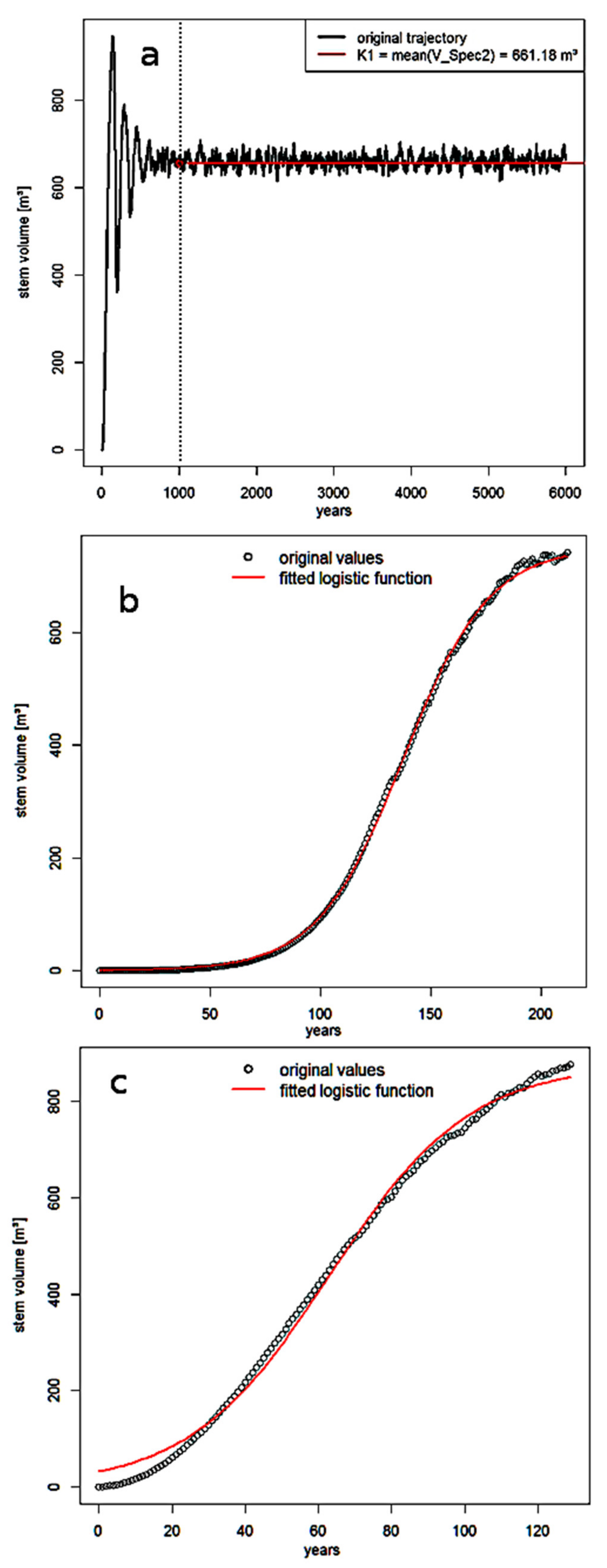
2.3. Parameterization of the Lotka–Volterra (LV) Model from Simulation Experiments

The design of simple individual-level models that correspond, in the long-range limit, to the classical Lotka–Volterra model of competition has been the most common approach to provide evidence for the importance of short-range interactions and dispersal [2,4,60].

For example, Neuhauser and Pacala [4] applied a continuous-time Markov process to an integer lattice that is occupied either by “species 1” or “species 2” on all lattice points and that has no vacancies (i.e., the high-density limit). The community dynamics on the lattice were governed by (1) a mortality process that is dependent on the conspecific density (multiplied by an intra-specific competition coefficient) and the heterospecific density (multiplied by an inter-specific competition coefficient), and (2) a reproductive replacement of death that is proportional to the densities of the two species weighted by their specific fecundities. A shift from local to global processes was achieved in the model by including more and more distant individuals as neighbors of a focal tree in respective density calculations. Overall, this approach is elegant, because the operation on the high-density limit avoids complications related to intrinsic growth rates (by ignoring them) and carrying capacities (by simplifying them to the total number of lattice points for both species).

The comparison of field-calibrated individual-based models, which simulate birth, growth, and death processes, and their likewise field-calibrated counterparts in the long-range limit (i.e., mean-field models) served the same objective as above [2,5,12,61]. However, with the exception of Pacala and Silander Jr. [61] (cited in 2), the calibrated mean-field models did not correspond to the Lotka–Volterra equations. Gathering LV parameters from the field, on the other hand, has turned out to be difficult (e.g., [62]) and is generally considered to be tedious, because single species, as well as neighbor removal experiments, in natural communities or mutual invasion experiments in spatially designed communities are required for this [63,64].

We avoided these difficulties here by following Pacala and Levin [2] and we adopted the approach to estimate intra-/inter-specific competition coefficients and other LV parameters from (manipulative) experiments in the IBM. Carrying capacities and intrinsic growth rates are readily obtained from single-species simulation experiments. Competition coefficients for the LV-model are readily available from community simulation experiments conducted with IBMs, because individual plants record competition from intra- and inter-specific neighbors at each time interval in these models.

Basically, the settings selected for the individual-based simulations should ensure that we achieved the simplification of environmental assumptions of the LV model in the long run (spatial and temporal homogeneity, no larger trophic structure, [28]). The biotic assumption that organisms are identical through time [28] is likely satisfied while the populations are in the steady-state and exhibit a constant size and age structure. However, the second biotic assumption of homogeneous unstructured populations, the so-called mean-field assumption, has to be carefully tested in the IBM simulation runs. Additionally, the approach as a whole requires us to critically evaluate the matching/scaling of individual-based processes contained in MesoFON and those contained in the LV model. We provide such an assessment in the following discussion.

Single-species experiments: We conducted single-species simulation experiments with the MesoFON model to parameterize the monospecific logistic growth curve of stem volume integrated over time t:

$${\mathrm{V}}_{\mathrm{i}}=\frac{{\mathrm{K}}_{\mathrm{i}}·{\mathrm{V}}_0·{\mathrm{e}}^{{\mathrm{r}}_{\mathrm{i}} · \mathrm{t}}}{{\mathrm{K}}_{\mathrm{i}}+{\mathrm{V}}_0·({\mathrm{e}}^{{\mathrm{r}}_{\mathrm{i}} · \mathrm{t}}-1)}$$

(9)

where V_i is the stem volume of species i at time t, V₀ is the initial stem volume for that species, K_i is the species-specific carrying capacity, and r_i is the stem volume growth rate.

All former entities are defined in units of m³ ha⁻¹, while the last is given in m³ ha⁻¹ yr⁻¹.

In principle, because of its sigmoidal form, the Shugart function that governs the stem diameter growth of an individual tree in the MesoFON Equation (2) might scale up to a logistic population growth. Indeed, stand volume trajectories of the JABOVA model (which also relies on the Shugart function) has repeatedly shown compliance with logistic growth, but other forms of population growth have also been reported [47].

Two separate simulation runs were conducted using the single species: (1) one underlying random global and (2) one underlying natural localized propagule dispersal. Equation (9) was fitted to the initial colonization phase where saplings grew almost in synchrony. We used the probabilistic optimization routine of the simulated-annealing method SANN within the optim-function of the statistical software R to fit the data [65]. We adjusted two of the three SANN control parameters following recommendations given by Cortez [66]. The initial temperature T was raised to 1000 to ensure that SANN operates as a global parameter search method. The maximum number of iterations was increased to 100,000 in order to enable convergence in the localized seed dispersal treatment. The resulting models were evaluated visually because SANN does not produce a goodness-of-fit measure (other than the residual sum of squares RSS).

Additionally, we recorded long-term mean values of the stem volume (K_i), the population size (K_i,indiv), and the average individual-based intra-specific competition (α_ii,indiv) from the MesoFON simulation runs. These annual recordings commenced in simulation year 1000 and are representative of the steady-state phase of population dynamics (with constant tree size structure). The multiplication of α_ii,indiv by K_i,indiv and the division by K_i produces the volume-specific α_ii for the monoculture, which can then be compared with α_ii, values achieved in the community.

Community experiments: Additionally, we carried out simulation experiments with a community consisting of both species. The purpose of the experiments was to verify that the two identical species can stably coexist in the individual-based model. The goal was to parameterize the intra- and inter-specific competition coefficients using annual competition recordings of the individual trees in the IBM. Separate MesoFON simulation runs were conducted such that the underlying community was formed by random global or natural localized propagule dispersal. In order to cover the full range of species compositions, without risking extinction of one species by chance, we initialized the runs with 15/735 and 735/15 saplings per hectare with Rhizophora spec. 1 and 2. We restricted data collection to the steady-state phase of the community dynamics (>500 yrs) in those experiments.

Before we outline the methodology used for data analysis, we introduce the set of differential equations that comprises the competitive LV-model, commonly based on population sizes [67,68,69]. We avoid difficulties related to size differences between species by defining the LV-model in terms of the stem volume per hectare as a proxy for the most suitable “common currency,” i.e., biomass per hectare. As Lotka (1925) [6] stated, users are free to switch units in the equations. The logistic growth equations for the interaction of species 1 and 2 are as follows:

$$\frac{{\mathrm{dV}}_1}{\mathrm{dt}}={\mathrm{r}}_1{\mathrm{V}}_1(1-\left({\mathrm{V}}_1+\frac{{\mathsf{\alpha }}_{1\leftarrow 2}}{{\mathsf{\alpha }}_{11}}{\mathrm{V}}_2\right)/{\mathrm{K}}_1)$$

(10)

$$\frac{{\mathrm{dV}}_2}{\mathrm{dt}}={\mathrm{r}}_2{\mathrm{V}}_2\left(1-({\mathrm{V}}_2+\frac{{\mathsf{\alpha }}_{2\leftarrow 1}}{{\mathsf{\alpha }}_{22}}{\mathrm{V}}_1\right)/{\mathrm{K}}_2)$$

(11)

where:

• r₁ and r₂ denote the intrinsic volume-specific growth rates for species 1 and 2 in m³ ha⁻¹ yr⁻¹, respectively;
• V₁ and V₂ represent the respective stem volumes in m³ ha⁻¹;
• K₁ and K₂ are the respective carrying capacities, also given in m³ ha⁻¹;
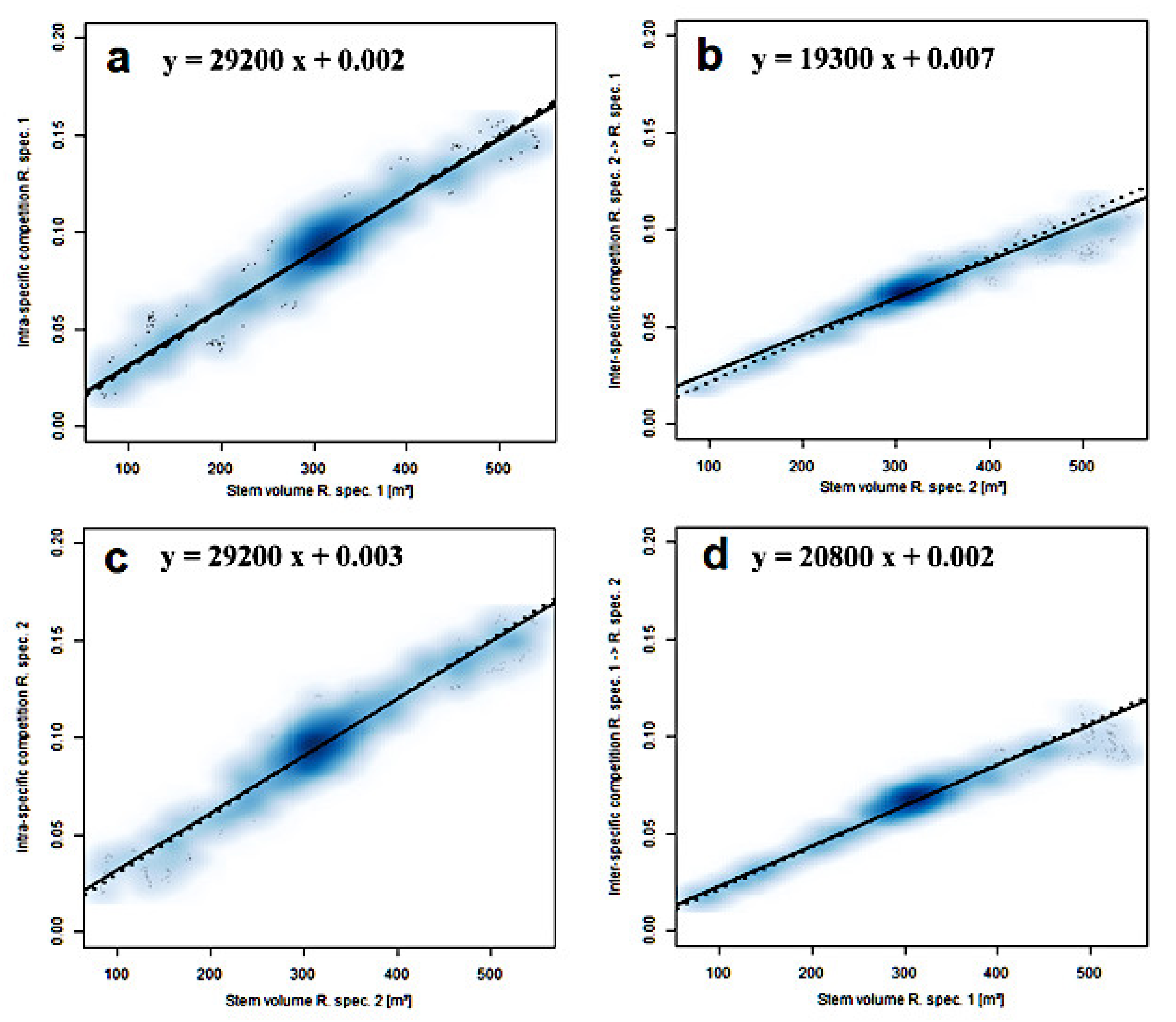
• α_1←2 is the inter-specific competition coefficient of species 2 on species 1;
• α_2←1 is the inter-specific competition coefficient of species 1 on species 2;
• α₁₁ and α₂₂ are the intra-specific competition coefficients of species 1 and 2, respectively.

Similar to the simple IBM of Neuhauser and Pacala [4], all processes included in our model under the chosen scenario conditions, namely fecundity, consisting of propagule production and sapling establishment, tree growth, and death from competition (except for natural death due to tree age), are density-dependent in a simple manner, and, thus, MesoFON is supposed to correspond in the long-range limit to the Lotka–Volterra model. The question of whether the distances of competitive interaction and/or propagule dispersal effective in the field-calibrated model are sufficiently long-ranged is addressed in this study.

The derivation of competition coefficients from simulations is described as follows: MesoFON provides the intra- and inter-specific competition that an average individual tree experiences as a derived system state variable. This normalized competition reflects the fractional growth reduction due to competition exhibited by the average tree. We multiply these individual-based competition coefficients by the stem volume of the respective species to produce the population-wide competition coefficients. Each of these coefficients was subsequently plotted against the stem volume of the species that affects that coefficient, and we then applied linear regression techniques to determine each volume-specific competition coefficient used in Equations (10) and (11). The linear regression allowed us to validate whether the mean field assumption that underlies the LV-model was satisfied by the IBM. The mean field assumption states “that individual organisms encounter one another in proportion to their average abundance across space” [3]. We verified the assumption here by confirming that those population-wide competition coefficients (e.g., α_ii $·$ V_i) were proportional to the stem volumes (e.g., V_i) along the respective isoclines. Due to the large samples we took in the simulation runs (≈2 × 7000 simulation years, ≈600 trees), we refused to apply statistical tests on the parameters of the linear regressions in the verification (compare Lin et al. [70] for statistical consequences of the large sample problem). Instead, we compared the robust regression having a nonzero intercept with a robust regression through the origin, and we assumed the mean-field assumption to hold when differences among the regressions were hardly visible. The robust regression was chosen to remove the influence of several outliers recorded outside the isocline range. Additional normal linear regression was used to obtain an R² goodness-of-fit measure.

The four possible competitive outcomes of the two species case are commonly determined graphically by the cardinal points (intersections with the axes) of the two species-specific isoclines, in the phase-plane diagram graphing V₂ vs. V₁. The zero growth isoclines are identified by setting Equations (10) and (11) to zero.

The “stable coexistence at equilibrium” occurs when (K₁ α₁₁/α_1←2) > K₂ and (K₂ α₂₂/α_2←1) > K₁. As we deal with identical species in this study and as we can assume that K₁ = K₂, these inequalities can be simplified to: α₁₁ > α_1←2 and α₂₂ > α_2←1; these relations are interpreted as the intra-specific competition must be greater than the inter-specific competition for the stable equilibrium to exist.

This scenario arises when inter-specific crown plasticity lowers the inter-specific competition sufficiently. On the other hand, if the species are identical, compete only for a single light resource, and all LV assumptions hold, we are on the nonspatial single-resource hyperbola in the LV parameter space [60] at the point where all competitive coefficients equal 1, and the scenario is, thus, only neutrally stable [28].

We present all results of the LV-analysis by way of specially adapted and highly illustrative phase-plane diagrams (Figures 5 and 7). The R-script used to draw these diagrams was modified after Poisot (2014) [71]. The black arrows located at grid points of the diagrams point in the direction of the local community shift, while the color scheme ranging from yellow to red indicates ascending rates of community change. Isoclines for the respective species are added to the diagram in the traditional way. Moreover, original data points are depicted as a smoothed scatter in the background. If the shape of the smoothed scatter suggested the existence at a classic equilibrium point, we fitted a multivariate adaptive regression spline (MARS) to the original data because MARS supports a bending in the data. The adaptive regression spline was retained if the value of its adjusted R² was superior. Otherwise, a major axis regression was fitted. Multivariate adaptive regression splines were constructed using the earth-package in R [72], whereas major axis regression models were constructed using the smatr-package in R [73]. In any case, graphs of the fitted model were added to the phase-plane diagram. When we found evidence for stable coexistence, we also plotted the means and standard deviations of the stem volumes at equilibrium (derived from a run with initial sapling numbers of 325/325 per hectare).

A summarizing workflow diagram of this study is provided in Appendix B, Figure A1.

3. Results

3.1. Community Dynamics in the Individual-Based Model

The two identical Rhizophora species that were designed to avoid each other’s competition were able to stably coexist in the individual-based model regardless of the dispersal regime. This is shown clearly in the stem volume trajectories of the runs (compare Figure 2).

In runs initialized with equal sapling numbers, the computed stem volumes were (1) ${\overline{\mathrm{V}}}_1=309.36\pm 17.17{ \mathrm{m}}^3{ \mathrm{ha}}^{-1}$ and ${\overline{\mathrm{V}}}_2=314.79\pm 17.17{ \mathrm{m}}^3{ \mathrm{ha}}^{-1}$(mean ± standard deviation with random dispersal), and (2) ${\overline{\mathrm{V}}}_1=318.50\pm 17.35{ \mathrm{m}}^3{ \mathrm{ha}}^{-1}$ and ${\overline{\mathrm{V}}}_2=294.43\pm 17.96{ \mathrm{m}}^3{ \mathrm{ha}}^{-1}$ (mean ± standard deviation with local dispersal). Therefore, the constancy amounted to 18.0 and 18.3 (or 18.15 on average) in the random dispersal treatment and to 18.4 and 16.4 (or 17.4 on average) with local dispersal. The results qualitatively support the classical competition theory proposed by Lotka and Volterra.

As expected, localized dispersal did reduce the speed of community dynamics. Apparently, much more time was required after pulse perturbation to return to the equilibrium in the localized dispersal regime (≈2460 yrs), relative to the random dispersal treatment (≈540 yrs) (compare Figure 2). Likewise, the resilience has been estimated to about 1.83 × 10⁻³ m³ yr⁻¹ in the global dispersal treatment compared to about 0.41 × 10⁻³ m³ yr⁻¹ with local dispersal. Of course, the question arises regarding which mechanisms caused this difference. We hope to clarify this question with the Lotka–Volterra parameterizations in the next sections.

3.2. Lotka–Volterra Parameters from Single-Species Experiments

This type of experiment was used to parameterize V₀, r_i, K_i, and the intra-specific competition coefficient α_ii.

Table 1. Lotka–Volterra Parameters.

a	Treatment	r1 (×10−2) [m3 ha−1 yr−1]	K1 [m3 ha−1]	V0 [m3 ha−1]	RSS (×10−3)
	Random Dispersal	5.119	752.42	0.66	6.76
	Natural Dispersal	5.201	878.35	31.93	46.76
b	Treatment	K1 [indiv. ha−1]	K1 [m3 ha−1]	α11,indiv (×10−4)	α11 (×10−4)
	Random Dispersal	822.02	621.72	1.98	2.62
	Natural Dispersal	831.54	617.42	1.93	2.60
c	Treatment	α11 (slope) (×10−4)	α11 (intercept)	R2	α1<-2 (slope) (×10−4)	α1<-2 (intercept)	R2
Plasticity	Random Dispersal	2.92	0.002	0.922	1.93	0.007	0.932
	Natural Dispersal	1.75	0.066	0.874	1.41	0.001	0.918
	Treatment	α22 (slope) (×10−4)	α22 (intercept)	R2	α2<-1 (slope) (×10−4)	α2<-1 (intercept)	R2
	Random Dispersal	2.92	0.003	0.916	2.08	0.002	0.937
	Natural Dispersal	1.66	0.069	0.869	1.36	0.002	0.938
d	Treatment	α11 (slope) (×10−4)	α11 (intercept)	R2	α1<-2 (slope) (×10−4)	α1<-2 (intercept)	R2
Relaxation	Random Dispersal	2.67	−0.005	0.980	2.60	0.003	0.968
	Natural Dispersal	1.77	0.054	0.929	1.84	0.001	0.944
	Treatment	α22 (slope) (×10−4)	α22 (intercept)	R2	α2<-1 (slope) (×10−4)	α2<-1 (intercept)	R2
	Random Dispersal	2.66	−0.004	0.977	2.60	0.003	0.977
	Natural Dispersal	1.77	0.053	0.933	1.81	0.001	0.938

a: Parameters of the single-species logistic growth curve (Equation (2)), fitted with SANN; b: Parameters, assessed during the steady-state phase of single-species experiments; α_ii = individual-based (classical) intra-specific competition coefficient; c: Parameters, derived from robust linear regression of population-wide intra- and inter-specific competition vs. respective stem volume. R² values were obtained from normal regression.

a presents the results of the respective model fittings. A stem volume trajectory is displayed in Figure 3a. It is characterized by an initial re-colonization and an overshoot in both, of which the stem volume comprises even-aged trees, followed by a damped oscillation wherein the age similarity fades away and a steady state develops after 500 or 1000 simulation years, at the latest, in which tree size structure is constant and oscillation is absent except for some demographic stochasticity. We subsumed by definition the overshoot and the damped oscillation under the term re-colonization, and we differentiated this from the steady state.

Diagrams of the fitted models are shown in Figure 3b,c. The growth rate values r_i, 5.119 and 5.201 m³ ha⁻¹ yr⁻¹, of the two dispersal regimes were very similar. In contrast, the Rhizophora species carrying capacity with localized dispersal was 16.7% larger than the carrying capacity with global dispersal. The visual appearance of Figure 3b and the low residual sums of squares (RSS = 6.76) indicate that Equation (9) fitted the data in the random dispersal treatment very well. Based on the visual appearance of Figure 3c, the large value of V₀ = 31.93 m³ ha⁻¹, and the associated large RSS = 46.76, we can conclude that the logistic curve overestimated the low stem volumes and fitted the growth in the localized dispersal (initially slow, and then rapidly accelerating) in a less accurate manner.

The carrying capacities, recorded as long-term averages and representative of steady-state population dynamics, were much lower than those attained in the colonization phase, as described above (compare Figure 3a). The reductions in the random and the localized dispersal case were 17.4% and 29.7%, respectively (see Table 1b). As the competitive outcome unfolds in the steady-state phase, we restricted our LV-analysis to the carrying capacities realized in that phase. The only parameter that we retained from the initial colonization was the growth rate r_i, which does not influence competitive outcomes.

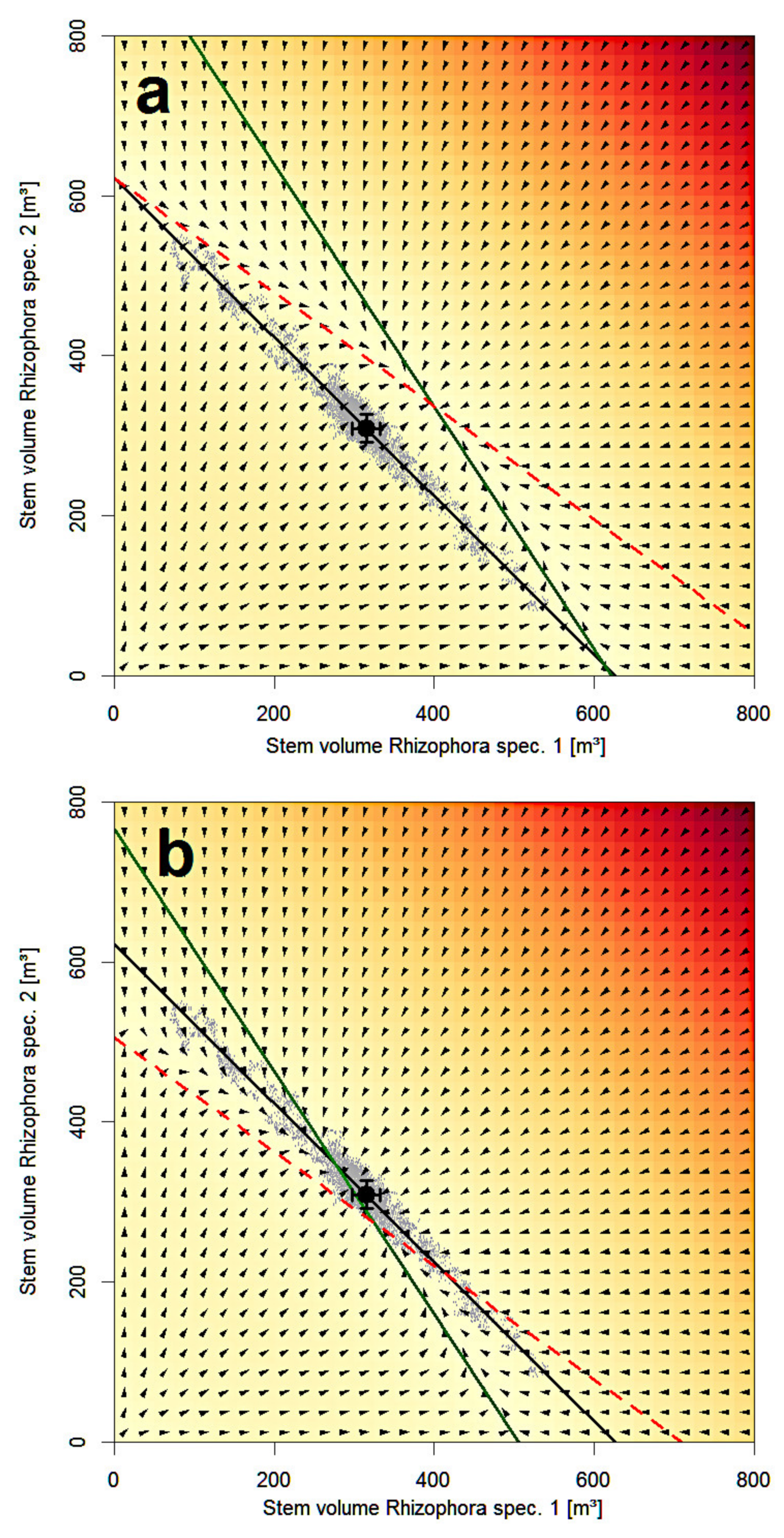
3.3. Lotka–Volterra Parameters from Community Experiments with Global Dispersal

Community experiments were conducted to determine values of the missing parameters α_1<−2 and α_2<−1, to achieve a full calibration of the Lotka–Volterra model. Even though these parameters were previously computed in the single-species experiments (compare Table 1b), we extended our analysis here to the intra-specific competition to confirm that the parameter values did not change relative to the values previously determined. As outlined in the “Materials and Methods” section, we obtained a volume-specific competition coefficient from the slope of a robust linear regression of the plot “population-wide competition vs. respective stem volume”. Table 1c contains the results of the linear regression; Figure 4a–d show corresponding diagrams with the fitted straight lines.

With values of R² ranging between 0.916 and 0.937, the linear models fitted the data very well. The intercepts of the linear regressions were very small, with the exception of α_1←2. As a result, differences between the robust regression with nonzero intercept, and the robust regression running through the origin, were hardly visible (compare Figure 4a,c,d), again with the exception of α_1←2 where the deviation was moderate but clearly visible (see Figure 4b). Hence, the visual inspection revealed that the mean field assumption was approximately achieved in the individual-based model.

Therefore, we ignored the minor intercepts and assumed that the slopes represent the competition coefficients. As slopes of the intra-specific models were much greater than their inter-specific counterparts (+39% and +51%, respectively), we did obtain a stable equilibrium.

Subsequently, we constructed a phase-plane diagram calculated from the slopes. Figure 5a shows the results of this classic but explorative LV-analysis.

The stable equilibrium of the LV-model is in qualitative agreement with the IBM, but the location of the equilibrium is distinct among the models. The LV-model predicted the equilibrium to be located at ${\widehat{\mathrm{V}}}_1=$ 398.94${ \mathrm{m}}^3{ \mathrm{ha}}^{-1}$ and ${\widehat{\mathrm{V}}}_2=$ 337.98${ \mathrm{m}}^3{ \mathrm{ha}}^{-1}$, whereas the equilibrium observed in the IBM was at ${\overline{\mathrm{V}}}_1=309.36\pm 17.17{ \mathrm{m}}^3{ \mathrm{ha}}^{-1}$ and at ${\overline{\mathrm{V}}}_2=314.79\pm 17.17{ \mathrm{m}}^3{ \mathrm{ha}}^{-1}$ (mean ± standard deviation). Consequently, with a value of 736.92 m³ ha⁻¹, the classic LV-model predicted the total stem volume at equilibrium to exceed or over-yield the carrying capacity of the single species at 621.72 by 115.20 m³ ha⁻¹, while, using the original data of the IBM, the equilibrium was at 624.15 m³ ha⁻¹ and, thus, very close to the capacity of the single species. This is confirmed by the major axis regression that fitted the original data very well (R² = 0.959). With an intercept of 622.13 ± 2.88 m³ ha⁻¹ and a slope of −0.9942 ± 0.0092 (mean ± 95% confidence interval), the graph connected the carrying capacities perfectly.

To overcome the defect of a falsely overyielding LV-model in further explorative analysis, we applied a non-overyielding Lotka–Volterra model that is defined by the following equation:

$$\frac{\mathrm{d}{\mathrm{V}}_{\mathrm{i}}}{\mathrm{d}\mathrm{t}}={\mathrm{r}}_{\mathrm{i}}{\mathrm{V}}_{\mathrm{i}}(1-({\mathrm{V}}_{\mathrm{i}}+\frac{{\mathsf{\alpha }}_{\mathrm{i}\leftarrow \mathrm{j}}}{{\mathsf{\alpha }}_{\mathrm{i}\mathrm{i}}}{\mathrm{V}}_{\mathrm{j}})/({\mathrm{K}}_{\mathrm{i}}·\sqrt{{\mathsf{\alpha }}_{\mathrm{i}\leftarrow \mathrm{j}}}/\sqrt{{\mathsf{\alpha }}_{\mathrm{i}\mathrm{i}}}))$$

(12)

As Figure 5b illustrates, the non-overyielding model matched the individual-based equilibrium far better than the classic model did. With ${\widehat{\mathrm{V}}}_2=$ 274.40${ \mathrm{m}}^3{ \mathrm{ha}}^{-1}$ and $\widehat{{\mathrm{V}}_1}=$ 3$23.89{ \mathrm{m}}^3{ \mathrm{ha}}^{-1}$, the supposed model did under-yield slightly by 23.43 m³ ha⁻¹.

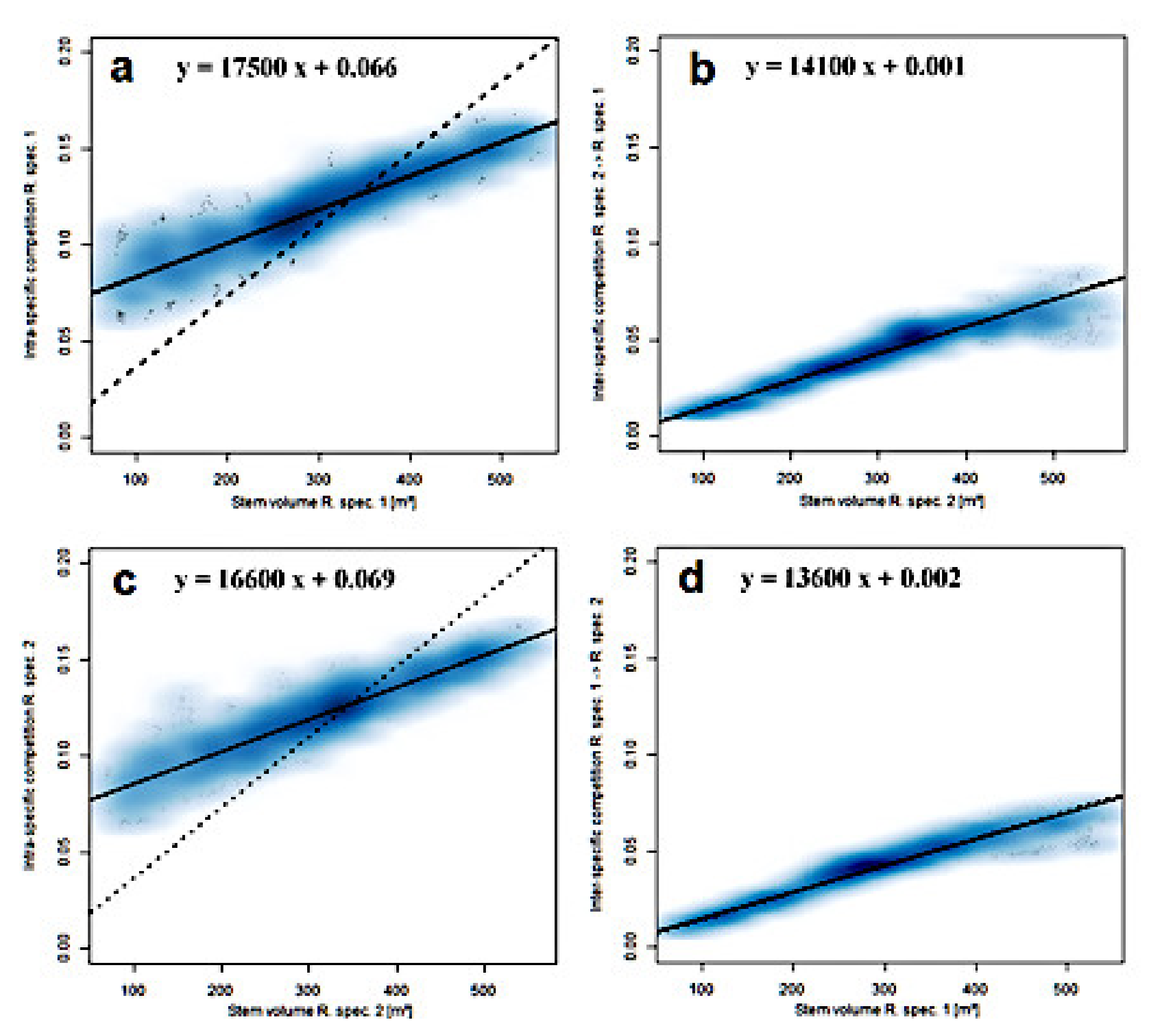
3.4. Lotka–Volterra Parameters from Community Experiments with Localized Dispersal

According to the stem volume trajectories of the MesoFON simulation runs, the equilibrium was obtained much later with the localized dispersal, and, therefore, the community was likely less resilient (see Figure 2). The derivation of the LV-parameters from the community experiments with local dispersal should clarify the underlying mechanisms.

Once again, we fitted robust linear regression models to the plots “population-wide competition vs. respective stem volume” to obtain volume-specific competition coefficients. Table 1c illustrates the results of the linear regression; Figure 6a–d show corresponding diagrams with the fitted straight lines.

The values of R² ranged from 0.874 to 0.938, indicating a good fit of the normal linear regression. However, in the case of localized dispersal, the slopes of both the intra- and inter-specific cases were much lower than the corresponding slopes for the random dispersal cases, but intra-specific slopes were still larger than the inter-specific slopes. The intercepts of the robust regression in the inter-specific cases were again close to zero. Similarly, differences between the robust regression with a nonzero intercept and the robust regression passing through the origin were hardly visible in the inter-specific diagrams of Figure 6b,d.

In contrast, robust regressions in the intra-specific cases had large intercepts. Such an intercept represents a competition that is inversely proportional to stem volume and converges to zero at infinity. We factored in the intercept by averaging the corresponding volume-specific competition above 100 m³ ha⁻¹, adding this value to the constant intra-specific competition value of the slope. Even though this is a conservative procedure, it raised intra-specific over inter-specific competition so dramatically that the resulting stable equilibrium in the exploratively applied classic LV-model (diagram not shown) greatly over-yielded the carrying capacity of the species at 617.42 m³ ha⁻¹, and the equilibrium observed in the IBM specified by ${\overline{\mathrm{V}}}_1=318.50\pm 17.35{ \mathrm{m}}^3{ \mathrm{ha}}^{-1}$ and ${\overline{\mathrm{V}}}_2=294.43\pm 17.96{ \mathrm{m}}^3{ \mathrm{ha}}^{-1}$ (mean ± standard deviation), or at 612.93 m³ ha⁻¹, in total. The location of the observed equilibrium is confirmed by the major axis regression that fitted the original data very well (R² = 0.983). With an intercept of 610.56 ± 0.88 m³ ha⁻¹ and a slope of −1.0044 ± 0.0028 (mean ± 95% confidence interval), the graph connected the carrying capacities almost perfectly. In contrast, MARS did not provide meaningful results.

If we exploratively applied the non-overyielding Lotka–Volterra model instead, we were again confronted with consequences of the large difference between the intra- and the inter-specific competition; in this case, the equilibrium exhibited a strong under-yield of the carrying capacities, with a large distance between the axis intersections of the isoclines (see Figure 7a). This did not correspond to observed community dynamics.

To address the issue in further exploration, we made a major assumption: We separated intra-specific competition into an effective mean-field part (i.e., the competition coefficient determined by the slope alone) and ignored the part that we believe reflects the inner-cluster competitive processes and does not influence the competitive outcome (i.e., the corresponding intercept). As Figure 7b shows, this approximation resulted in the convergence to the observed equilibrium at a rate that was close to the observed rate.

4. Discussion

The two identical Rhizophora species that were designed to avoid each other’s competition were able to stably coexist in the individual-based model regardless of the dispersal regime. In our study, we avoided artificial methods to stabilize the community, such as external seed input or large plot dimensions [14]. Hence, the stable coexistence observed here is genuine.

The carrying capacities, recorded as long-term averages and representative of steady-state population dynamics, in the global and localized dispersal treatment were 17.4% and 29.7% lower than those attained in the early colonization phase. During initial colonization, the even-aged monoculture stands drove along the self-thinning line [74], therefore attaining the highest possible stem volumes, and they passed through an overshoot. An initial overshoot of a forest stand’s biomass followed by a damped oscillation toward a lower steady state has been reported as a potential outcome of forest gap models, such as JABOWA, which have the Shugart growth function in common with MesoFON; the phenomenon is known to be a consequence of lagged mortality and/or lagged regeneration (Borrmann and Likens 1979a,b, Peet 1981 cited in [47]). In accordance with that, a tree dies in MesoFON only when slow diameter growth persists for five consecutive years (compare Section 2.1.5) and generative reproduction does not start until a certain tree age is reached (i.e., when the crown surface area A is sufficiently large that the no. of propagules = f_red × D × A ≥ 1, compare Section 2.1.1). Surpassing standing stocks after (re-)colonization are acknowledged behaviors of mangrove forests (Twilley, personal communication). As several assumptions of the LV model are unlikely to be met during the overshoot and oscillatory phases (temporal homogeneity, mean-field assumption: outliers in Figure 4 and Figure 6 likely originated from these phases), the validity of the Lotka–Volterra model is constrained to the steady-state phase that commences of the order of 500 years after, what we consider, a complete canopy removal by a large-scale disturbance event at the beginning of the simulation (compare Figure 2a). Given the typical frequencies of large-scale mangrove disturbance by hurricanes, this leads to the question of whether the Lotka–Volterra equations are applicable to mangrove forests at all. Rhizophora mangle, even though considered as a sensitive species, is severely damaged only when sustained hurricane wind speeds exceed 177 km/h (Category 3 to 5 hurricanes, [75]). For Florida, Costanza et al. (2008) [76] report return periods of 6, 26, and 77 years for Category 3, 4, and 5 hurricanes to hit coastal wetlands, respectively. Based on these values, it seems appropriate to answer the above question with “No.” However, one should bear in mind that not all the mangrove area being hit by a hurricane would be damaged severely. Even the large Category 5 hurricane Andrew damaged >90% of the Everglades mangrove vegetation on a coastal transect only in the 40 km eyewall zone and >70% in the eyewall zone, including a 40 km wide band north of it [77].

Nevertheless, as we characterized R. mangle as a typical pioneer tree species, we may also look at forest disturbance more broadly. In their global review on this topic, Folking et al. (2009) [78] list the recurrence of major large-scale forest disturbance types: fire (spatial scale: <1 to >10⁴ km²): recurrence <10–1000 years; hurricanes (10³–10⁵ km²): 15–200 years, flooding (10–10⁴ km²): 50–100 years. These figures suggest that the LV model might be applicable to less fire-prone forests and to forests rarely impacted by hurricanes if we take into account the above argument regarding the eyewall zone.

As the mean field assumption was approximately achieved in the individual-based model, we consider the effects of crown plasticity combined with random dispersal as an archetype for localized behavior. This is outlined in the following discussion. The mean-field assumption is generally considered valid when the environment is homogeneous, when organisms are well mixed, and when their interactions are over long distances [3]. In our simulations, the environment was homogeneous, with random dispersal, and the community was well mixed even though the trees were sessile. However, the application of the local interaction, present in all the MesoFON runs, should have resulted in a fine-scale spatial structure and a “plant’s eye view” that differs from large-scale spatial averages [79]. However, as long as the alteration of spatial structure does not scale up (see below) and a sufficiently large number of trees take a broad sample of the density, the composition of the average neighborhood is a “miniaturized” image of the global density average (as in configuration-field models, [80]). As the mean field was approximately achieved, we ignored the minor intercepts and assumed that the slopes represent the competition coefficients. As slopes of the intra-specific models were much greater than their inter-specific counterparts (+39% and +51%, respectively), we did obtain a stable equilibrium. The suggested mechanism is: when displaced, the community is returned to the stable equilibrium by the high mortality of one species due to the higher intra-specific competition, just as a rolling ball is returned to the bottom of a deep bowl by the moment of the gravitational force (compare Figure 8a).

The non-overyielding LV model matched the individual-based equilibrium in the global dispersal treatment far better than the classic model and did under-yield only slightly. The latter result may be explained by the fact that the accuracy of the equation is restricted for ratios of intra- vs. inter-specific competition sufficiently close to 1. A mechanistic explanation for this “goal-oriented” LV-model is suggested by the comparison of competition coefficients attained in single-species and community experiments. In accordance with our expectations, inter-specific coefficients in the community (1.93 and 2.08 × 10⁻⁴) are far below those of single-species experiments (2.62 × 10⁻⁴), but concurrently, intra-specific coefficients (both 2.92 × 10⁻⁴) are above their single-species counterparts. Both alterations have certainly contributed to the strong stabilizing effects of crown plasticity. While the former change represents a decrease of approximately 27%, the latter represents an 11% increase in the competition. We thus conclude that it is necessary to estimate intra-specific competition coefficients in both community and single-species experiments, because they are not invariant and their comparison contributes to the mechanistic understanding of the underlying processes. Yet, the mechanistic interpretation of the pattern is: the implemented inter-specific neighborhood avoidance moved heterospecific trees apart from each other and pushed conspecifics together. Based on this result, the linear trend of the original data and the occurrence of a stable equilibrium at carrying capacity seem reasonable.

However, even though the constructed non-overyielding LV model provides a good prediction of the equilibrium and the speed approaching the equilibrium (determined by the width of the triangles between isoclines), it implies the occurrence of bending at the equilibrium and a reduction in the apparent carrying capacities. Both implications seemed to be absent from the original data, because MARS did not provide reasonable results. Moreover, the latter implication conflicts with the carrying capacity measured in the single-species experiments. Yet, we cannot rule out that the properties of the LV-model alter when one of the species becomes rare (data not shown). According to the discussion in Loreau (2010) [64], a non-overyielding equilibrium occurs only when isoclines are nonlinear and convex functions. Apparently, this was not the case here. From the perspective of an LV-modeler, a linear trend, as observed in the original data of the individual-based simulations, is not feasible.

In summary, we found that a non-overyielding model, rather than the classical Lotka–Volterra model, approximated most of the competitive behavior observed in the MesoFON model, even though the LV-model was not fully compatible with the IBM. The inter-specific crown plasticity acted as a strong stabilizing mechanism. Given the mean field assumption was approximately satisfied, it represented largely a localized process.

The approximate validity of the mean-field assumption was in line with mathematical descriptions given by Neuhauser and Pacala [4], but more importantly, it is in accordance with the work of Adams et al. [12], who stated that competitive interactions in real temperate forests are less local than those reported to cause species separation in theoretical studies conducted with spatially explicit model types other than field-calibrated IBMs (e.g., continuous-time Markov process [4]; interacting particle systems, stochastic point processes, noncontiguous patch models [60]).

Localized seed dispersal is generally considered an equalizing coexistence mechanism [14,15,16,17] that, by definition, slows the community dynamics but does not alter the competitive outcome among the species. In this study, we have analyzed two community stability properties, namely constancy and resilience. Both were affected by localized dispersal in the same direction, but to a different extent. While local dispersal lowered the constancy only slightly by about 4%, it reduced the resilience about 4.5-fold. The decline in resilience is consistent with the definition of an equalizing mechanism, even though this does not necessarily mean that the community is less stable with local dispersal. We expect a similar drop in the antagonist of resilience, the resistance [56], because this would lead to delayed responses, as described in the above definition. Resistance, however, is almost impossible to measure in the field [56], Unfortunately, this prevented us from including resistance in our analysis. Based on the gained understanding, we recommend defining resistance henceforth as the rate of a press perturbation that does not yet lead to a significant change in the community at the reference state, and determining resistance in future IBM studies by assigning increasing numbers of species 1 trees to species 2 until the threshold that leads to a change is passed. Nonetheless, the lower resilience and the presumably delayed community responses contradict the expectation that stabilizing and equalizing mechanisms act in the same direction and that both contribute to the coexistence of species.

However, in this study, plotting “population-wide competition vs. stem volume” provided evidence of the following mechanism: Individuals in a large portion of the plot area formed conspecific clusters and left the competitive race. The strength of intra- and inter-specific competition, as well as their difference, diminished, concurrently, in the inter-cluster mean field. When displaced, the locally dispersed community slowly returned to the stable equilibrium by the higher mortality of one species due to the slightly higher apparent intra-specific competition, just as a rolling ball is slower when returned to the bottom of a shallow bowl compared to the bottom of a deep bowl by the moment of the gravitational force (compare Figure 8b). In contrast to crown plasticity, local dispersal is a process that scales up to larger spatial dimensions.

Implications of the results for field surveys: Our case study revealed that an excess of inter-specific over intra-specific crown displacement facilitates the coexistence of two typical pioneer tree species ([81,82] and Material and Methods section). However, as we pointed out in the introduction, the artificiality of our critical case (identical species exhibiting solely inter-specific crown plasticity) requires us to evaluate the implications of the obtained results for field surveys. Hence, in the following, we first address the question: Have any field studies provided evidence of excessive inter-specific crown plasticity and positive implications on species coexistence?

Plants, in general, are known to respond pro-actively and differently to the shade of different neighboring species via their red/far-red (R/FR) spectral perception system [83]. In accordance with that, a wide range of alterations in crown architecture at various spatial scales was found between mixed and pure stands in terrestrial laser scanning studies [84,85,86]. In addition, conspecific neighbors were often found to be stronger competitors than heterospecific neighbors [87,88,89].

The most direct evidence of stronger inter-specific plasticity, however, is offered by the survey on the variability of crown projection area in inter- vs. intra-specific environments conducted by Pretzsch et al. (2017) [29] on 80-year-old permanent plots containing mixed stands of European beech (Fagus sylvatica L.) x Sessile oak (Quercus petraea (Matt.) Liebl.) and pure stands of those two species. With 2326 beech and 1959 oak trees per hectare (4285 ha⁻¹ in total), mixed stands comprised a much larger tree density than pure stands of Fagus sylvatica (3173 ha⁻¹) and of Quercus petraea (2888 ha⁻¹), respectively. This occurred partly at the expense of tree size [29]. Crowns of individual oak trees responded mostly with a wider projection area per stand area (cpa/sa, the latter derived from Voronoi tessellation) to the crowding in the mixed stands (0.90 in pure to 1.39 in mixed stands) and, to a lesser extent, with a rise in normalized crown displacement (3.10 in pure to 3.30 in mixed stands). In contrast, beech trees responded to it primarily with an exceeding surge in normalized crown displacement (4.0 in pure to 7.4 in mixed stands) and less so with an increase in cpa/sa (1.32 in pure to 1.48 in mixed stands). It might be due to the overall high packing density that the late-successional and shade-tolerant species was more plastic than the mid-successional light-demanding species in this study, whereas in most other studies, the opposite ranking was observed [90,91,92]. However, because crown displacement had been divided by d_1.37 and, thus, normalized to equal tree size (29), it is highly likely that European beech and, even though less likely, that Sessile oak expressed stronger inter-specific crown plasticity values. As our study suggests, a stronger inter-specific crown displacement opens a window for stable coexistence, but its realization will likely depend on the difference between carrying capacities of the species and the excess of inter-specific over intra-specific crown plasticity for both species—irrespective of whether early- or late-successional species are more plastic. The carrying capacity of European beech, in particular, seems to exceed that of Sessile oak by far, as intensive forest management or frequent disturbances are needed to prevent Sessile oak from extinction [93]. If, in turn, the carrying capacities of early- and late-successional tree species resemble one another more closely, excessive inter-specific crown plasticity could represent an alternative coexistence mechanism beyond the competition-colonization tradeoff in the disturbance-mediated Mosaic cycle [28,46,64,94]. To the best of our knowledge, such a mechanism has not been studied yet. Its substantiation will require the careful interaction of field research and modeling efforts.

The second question we would like to address is the specification of the first question to mangroves. This is not an easy task, because field research on mangrove crown plasticity is still in its infancy. Vovides et al. (2018) [95] were the first researchers and, so far, the only ones who investigated the crown displacement of mangrove species. They measured stem positions and crown projection areas in eight cardinal directions for canopy and sub-canopy trees of Neotropical mangrove species (R. mangle, Laguncularia racemosa (L.) C.F.Gaertn., A. germinans) in Mexican mangrove forests along a salinity gradient. Wind direction/intensity exerted a strong influence on the crown displacement of canopy trees at all salinities, but for sub-canopy trees, a change in driving forces of crown displacement along the salinity gradient was detected: In the dense canopies at low salinity, neighborhood avoidance prevailed as a driver, whereas in sparse canopies at high salinities, crown overlap and neighborhood avoidance subsided—presumably due to stronger below-ground competition [95]. Among the species, the late-successional Avicennia germinans did exhibit the strongest crown plasticity—reminding us of the beech–oak case study described by Pretzsch et al. [29] (see above). Examining differences between inter- and intra-specific crown displacement and/or their implications for mangrove species coexistence was not among the objectives of Vovides et al. [95]. However, as these data are freely available on the worldwide web (compare the link in [95]), this could be readily addressed by comparing response strengths of crowns in heterospecific and monospecific neighborhoods or by allowing crown plasticity parameters in MesoFON to differ between species-specific neighborhoods and retrieve optimum values for them via Genetic Algorithms (compare Grueters et al., 2019 [23]).

5. Conclusions

In qualitative support of the LV-model, two identical Rhizophora species that avoid competition with one another by lateral crown displacement can stably coexist in the “small world” of a field-calibrated individual-based model with a homogeneous environment.

The mean-field assumption was approximately satisfied in the random propagule dispersal treatment. In spite of that, the classic Lotka–Volterra model that was calibrated from the IBM simulation runs was invalid. Rather, the “non-overyielding” LV-model provided a more accurate approximation of the competitive behavior observed in the IBM. The underlying mechanism possessed the following characteristics: The implemented inter-specific neighborhood avoidance moved heterospecific trees apart from each other, and it pushed conspecifics together. Inter-specific crown plasticity represents the archetype of a local process that exerts a strong stabilizing effect when it is combined with random dispersal.

Community dynamics were slowed by localized propagule dispersal. This delayed the time to reach equilibrium and, thus, the recovery time of the community. The underlying mechanism for this behavior was: Individuals in a large portion of the plot area formed conspecific clusters and left the competitive race. The competitive race took place in the inter-cluster mean field, where the strength of intra- and inter-specific competition, as well as their difference, diminished. Our results suggest that the community dynamics of field-calibrated individual-based models deviate from the behavior of a mean field if local competition and localized seed dispersal combine, but no deviation occurs when local competition operates in isolation.

In this study, we found that the dynamics of a field-calibrated IBM followed predictions of classical competition theory, rather than resource competition theory. As field-calibrated IBMs are resource-based and, thus, the competitive outcome in such models is implicitly mediated by the competition for resources, we conclude that classical competition mechanisms can override those of resource competition theory. This implies that more species are able to coexist in a plant community than predicted by resource competition theory.

References

1. Grimm, V.; Railsback, S.F. Individual-Based Modeling and Ecology; Princeton University Press: Princeton, NJ, USA, 2005; ISBN 9780691096667. [Google Scholar]
2. Pacala, S.W.; Levin, S.A. Biologically generated spatial pattern and the coexistence of competing species. In Spatial Ecology: The Role of Space in Population Dynamics and Interspecific Interactions; Princeton University Press: Princeton, NJ, USA, 1997; pp. 204–232. [Google Scholar]
3. Law, R.; Dieckmann, U.; Metz, J.A.J. Introduction. In The Geometry of Ecological Interactions: Simplifying Spatial Complexity; Cambridge University Press: Cambridge, UK; New York, NY, USA, 2000; pp. 1–6. ISBN 9780521642941. [Google Scholar]
4. Neuhauser, C.; Pacala, S.W. An Explicitly Spatial Version of the Lotka-Volterra Model with Interspecific Competition. Ann. Appl. Probab. 1999, 9, 1226–1259. [Google Scholar]
5. Pacala, S.W.; Deutschman, D.H. Details that matter: The spatial distribution of individual trees maintains forest ecosystem function. Oikos 1995, 74, 357. [Google Scholar] [CrossRef]
6. Lotka, A.J. Elements of Physical Biology; Williams & Wilkins Company: Baltimore, MD, USA, 1925. [Google Scholar]
7. Volterra, V. Variazioni e Fluttuazioni del Numero d’individui in Specie Animali Conviventi, Memoria del Socio Vito Volterra; Società Anonima Tipografica Leonardo da Vinci: Città di Castello, Italy, 1926. [Google Scholar]
8. Tilman, D. Resource Competition and Community Structure; Princeton University Press: Princeton, NJ, USA, 1982; ISBN 9780691083025. [Google Scholar]
9. Elser, J.J.; Bracken, M.E.S.; Cleland, E.E.; Gruner, D.S.; Harpole, W.S.; Hillebrand, H.; Ngai, J.T.; Seabloom, E.W.; Shurin, J.B.; Smith, J.E. Global analysis of nitrogen and phosphorus limitation of primary producers in freshwater, marine and terrestrial ecosystems. Ecol. Lett. 2007, 10, 1135–1142. [Google Scholar] [CrossRef] [PubMed] [Green Version]
10. Harpole, W.S.; Ngai, J.T.; Cleland, E.E.; Seabloom, E.W.; Borer, E.T.; Bracken, M.E.S.; Elser, J.J.; Gruner, D.S.; Hillebrand, H.; Shurin, J.B.; et al. Nutrient co-limitation of primary producer communities. Ecol. Lett. 2011, 14, 852–862. [Google Scholar] [CrossRef] [PubMed]
11. Wirtz, K.W.; Kerimoglu, O. Autotrophic stoichiometry emerging from optimality and variable co-limitation. Front. Ecol. Evol. 2016, 4, 131. [Google Scholar] [CrossRef] [Green Version]
12. Adams, T.; Ackland, G.; Marion, G.; Edwards, C. Effects of local interaction and dispersal on the dynamics of size-structured populations. Ecol. Model. 2011, 222, 1414–1422. [Google Scholar] [CrossRef] [Green Version]
13. Murrell, D.J. When does local spatial structure hinder competitive coexistence and reverse competitive hierarchies? Ecology 2010, 91, 1605–1616. [Google Scholar] [CrossRef] [Green Version]
14. Chesson, P. Mechanisms of maintenance of species diversity. Annu. Rev. Ecol. Evol. Syst. 2000, 31, 343–366. [Google Scholar] [CrossRef] [Green Version]
15. Stoll, P.; Prati, D. Intraspecific aggregation alters competitive interactions in experimental plant communities. Ecology 2001, 82, 319–327. [Google Scholar] [CrossRef]
16. Levine, J.M.; Murrell, D.J. The community-level consequences of seed dispersal patterns. Annu. Rev. Ecol. Evol. Syst. 2003, 34, 549–574. [Google Scholar] [CrossRef] [Green Version]
17. Barot, S. Mechanisms promoting plant coexistence: Can all the proposed processes be reconciled? Oikos 2004, 106, 185–192. [Google Scholar] [CrossRef] [Green Version]
18. Strigul, N.; Pristinski, D.; Purves, D.W.; Dushoff, J.; Pacala, S.W. Scaling from trees to forests: Tractable macroscopic equations for forest dynamics. Ecol. Monogr. 2008, 78, 523–545. [Google Scholar] [CrossRef] [Green Version]
19. Pacala, S.W.; Canham, C.D.; Saponara, J.; Silander, J.A., Jr.; Kobe, R.K.; Ribbens, E. Forest models defined by field measurements: Estimation, error analysis and dynamics. Ecol. Monogr. 1996, 66, 1–43. [Google Scholar] [CrossRef]
20. Grueters, U.; Seltmann, T.; Schmidt, H.; Horn, H.; Pranchai, A.; Vovides, A.G.; Peters, R.; Vogt, J.; Dahdouh-Guebas, F.; Berger, U. The mangrove forest dynamics model mesoFON. Ecol. Model. 2014, 291, 28–41. [Google Scholar] [CrossRef]
21. Berger, U.; Hildenbrandt, H. A new approach to spatially explicit modelling of forest dynamics: Spacing, ageing and neighbourhood competition of mangrove trees. Ecol. Model. 2000, 132, 287–302. [Google Scholar] [CrossRef]
22. Pretzsch, H. Forest Dynamics, Growth and Yield from Measurement to Model; Springer: Berlin, Germany; London, UK, 2009; ISBN 9783540883074. [Google Scholar]
23. Grueters, U.; Ibrahim, M.R.; Satyanarayana, B.; Dahdouh-Guebas, F. Individual-based modeling of mangrove forest growth: MesoFON—Recent calibration and future direction. Estuar. Coast. Shelf Sci. 2019, 227, 106302. [Google Scholar] [CrossRef] [Green Version]
24. Dahdouh-Guebas, F.; Hugé, J.; Abuchahla, G.M.O.; Cannicci, S.; Jayatissa, L.P.; Kairo, J.G.; Kodikara Arachchilage, S.; Koedam, N.; Mafaziya Nijamdeen, T.W.G.F.; Mukherjee, N.; et al. Reconciling nature, people and policy in the mangrove social-ecological system through the adaptive cycle heuristic. Estuar. Coast. Shelf Sci. 2021, 248, 106942. [Google Scholar] [CrossRef]
25. Yin, R.K. Case Study Research: Design and Methods, 4th ed.; Sage: Los Angeles, CA, USA, 2009; ISBN 9781412960991. [Google Scholar]
26. Flyvbjerg, B. Chapter 17: Case study. In The SAGE Handbook of Qualitative Research, 4th ed.; Denzin, N.K., Lincoln, Y.S., Eds.; Sage: New York, NY, USA, 2011; pp. 301–316. ISBN 9781412974172. [Google Scholar]
27. Ridder, H.-G. Case Study Research: Approaches, Methods, Contribution to Theory; Rainer Hampp: München, Mering, 2016; ISBN 9783957101754. [Google Scholar]
28. Grover, J.P. Resource Competition, 1st ed.; Chapman & Hall: London, UK; New York, NY, USA, 1997. [Google Scholar]
29. Pretzsch, H.; Forrester, D.I.; Bauhus, J. Mixed-Species Forests: Ecology and Management; Springer: Berlin, Germany, 2017; ISBN 978-3662545515. [Google Scholar]
30. Sengupta, R.; Middleton, B.; Yan, C.; Zuro, M.; Hartman, H. Landscape characteristics of Rhizophora mangle forests and propagule deposition in coastal environments of Florida (USA). Landsc. Ecol. 2005, 20, 63–72. [Google Scholar] [CrossRef]
31. Chen, R.; Twilley, R.R. A gap dynamic model of mangrove forest development along gradients of soil salinity and nutrient resources. J. Ecol. 1998, 86, 37–51. [Google Scholar] [CrossRef]
32. Levin, S.A.; Muller-Landau, H.C.; Nathan, R.; Chave, J. The ecology and the evolution of seed dispersal: A theoretical perspective. Annu. Rev. Ecol. Evol. Syst. 2003, 34, 575–604. [Google Scholar] [CrossRef]
33. Van der Stocken, T.; de Ryck, D.J.R.; Vanschoenwinkel, B.; Deboelpaep, E.; Bouma, T.J.; Dahdouh-Guebas, F.; Koedam, N. Impact of landscape structure on propagule dispersal in mangrove forests. Mar. Ecol. Prog. Ser. 2015, 524, 95–106. [Google Scholar] [CrossRef]
34. Sousa, W.P.; Kennedy, P.G.; Mitchell, B.J.; Ordóñez, B.M.L. Supply-side ecology in mangroves: Do propagule dispersal and seedling establishment explain forest structure? Ecol. Monogr. 2007, 77, 53–76. [Google Scholar] [CrossRef]
35. Van Speybroeck, D. Regeneration strategy of mangroves along the Kenya coast: A first approach. Hydrobiologia 1992, 247, 243–251. [Google Scholar] [CrossRef]
36. Cannicci, S.; Burrows, D.; Fratini, S.; Smith, T.J.; Offenberg, J.; Dahdouh-Guebas, F. Faunal impact on vegetation structure and ecosystem function in mangrove forests: A review. Aquat. Bot. 2008, 89, 186–200. [Google Scholar] [CrossRef]
37. Dahdouh-Guebas, F.; Koedam, N.; Satyanarayana, B.; Cannicci, S. Human hydrographical changes interact with propagule predation behaviour in Sri Lankan mangrove forests. J. Exp. Mar. Biol. Ecol. 2011, 399, 188–200. [Google Scholar] [CrossRef]
38. Tomlinson, P.B. The Botany of Mangroves, 1st ed.; Cambridge University Press: Cambridge, UK, 1994; ISBN 9780521466752. [Google Scholar]
39. De Ryck, D.J.R.; Robert, E.M.R.; Schmitz, N.; Van der Stocken, T.; Di Nitto, D.; Dahdouh-Guebas, F.; Koedam, N. Size does matter, but not only size: Two alternative dispersal strategies for viviparous mangrove propagules. Aquat. Bot. 2012, 103, 66–73. [Google Scholar] [CrossRef] [Green Version]
40. Van der Stocken, T.; De Ryck, D.J.R.; Balke, T.; Bouma, T.J.; Dahdouh-Guebas, F.; Koedam, N. The role of wind in hydrochorous mangrove propagule dispersal. Biogeosciences 2013, 10, 3635–3647. [Google Scholar] [CrossRef] [Green Version]
41. Van der Stocken, T.; Vanschoenwinkel, B.; De Ryck, D.J.; Bouma, T.J.; Dahdouh-Guebas, F.; Koedam, N.; Álvarez, I. Interaction between Water and Wind as a Driver of Passive Dispersal in Mangroves. PLoS ONE 2015, 10, e0121593. [Google Scholar] [CrossRef] [Green Version]
42. Van der Stocken, T.; Wee, A.K.S.; de Ryck, D.J.R.; Vanschoenwinkel, B.; Friess, D.A.; Dahdouh-Guebas, F.; Simard, M.; Koedam, N.; Webb, E.L. A general framework for propagule dispersal in mangroves. Biol. Rev. Camb. Philos. Soc. 2019, 94, 1547–1575. [Google Scholar] [CrossRef] [PubMed] [Green Version]
43. Hintze, C.; Heydel, F.; Hoppe, C.; Cunze, S.; König, A.; Tackenberg, O. D3: The Dispersal and Diaspore Database—Baseline data and statistics on seed dispersal. Perspect. Plant Ecol. Evol. Syst. 2013, 15, 180–192. [Google Scholar] [CrossRef] [Green Version]
44. Tamme, R.; Götzenberger, L.; Zobel, M.; Bullock, J.M.; Hooftman, D.A.; Kaasik, A.; Pärtel, M. Predicting species’ maximum dispersal distances from simple plant traits. Ecology 2014, 95, 505–513. [Google Scholar] [CrossRef] [PubMed] [Green Version]
45. Vittoz, P.; Engler, R. Seed dispersal distances: A typology based on dispersal modes and plant traits. Bot. Helv. 2007, 117, 109–124. [Google Scholar] [CrossRef] [Green Version]
46. Botkin, D.B.; Janak, J.F.; Wallis, J.R. Rationale, limitations, and assumptions of a northeastern forest growth simulator. IBM J. Res. Dev. 1972, 16, 101–116. [Google Scholar] [CrossRef]
47. Shugart, H.H. A Theory of Forest Dynamics: The Ecological Implications of Forest Succession Models; Springer: New York, NY, USA, 1984; ISBN 9783540960003. [Google Scholar]
48. Craine, J.M. Resource Strategies of Wild Plants; Princeton University Press: Princeton, NJ, USA, 2009; ISBN 978-0-691-13911-1. [Google Scholar]
49. Grams, T.E.E.; Andersen, C.P. Competition for resources in trees: Physiological versus morphological plasticity. In Progress in Botany; Springer: Berlin, Germnay, 2007; pp. 356–381. ISBN 3540368329. [Google Scholar]
50. Casper, B.B.; Jackson, R.B. Plant competition underground. Annu. Rev. Ecol. Evol. Syst. 1997, 28, 545–570. [Google Scholar] [CrossRef] [Green Version]
51. Huisman, J.; Weissing, F.J. Light-Limited Growth and Competition for Light in Well-Mixed Aquatic Environments: An Elementary Model. Ecology 1994, 75, 507–520. [Google Scholar] [CrossRef] [Green Version]
52. Borer, E.T.; Seabloom, E.W.; Gruner, D.S.; Harpole, W.S.; Hillebrand, H.; Lind, E.M.; Adler, P.B.; Alberti, J.; Anderson, T.M.; Bakker, J.D.; et al. Herbivores and nutrients control grassland plant diversity via light limitation. Nature 2014, 508, 517–520. [Google Scholar] [CrossRef] [PubMed]
53. Grimm, V.; Berger, U.; Bastiansen, F.; Eliassen, S.; Ginot, V.; Giske, J.; Goss-Custard, J.; Grand, T.; Heinz, S.K.; Huse, G.; et al. A standard protocol for describing individual-based and agent-based models. Ecol. Model. 2006, 198, 115–126. [Google Scholar] [CrossRef]
54. Grimm, V.; Berger, U.; DeAngelis, D.L.; Polhill, J.G.; Giske, J.; Railsback, S.F. The ODD protocol: A review and first update. Ecol. Model. 2010, 221, 2760–2768. [Google Scholar] [CrossRef] [Green Version]
55. Grimm, V.; Wissel, C. Babel, or the ecological stability discussions: An inventory and analysis of terminology and a guide for avoiding confusion. Oecologia 1997, 109, 323–334. [Google Scholar] [CrossRef] [PubMed]
56. Wilson, J.B.; Agnew, A.D.Q.; Roxburgh, S.H. The Nature of Plant Communities; Cambridge University Press: New York, NY, USA, 2019; ISBN 9781108482219. [Google Scholar]
57. Lehman, C.L.; Tilman, D. Biodiversity, Stability, and Productivity in Competitive Communities. Am. Nat. 2000, 156, 534–552. [Google Scholar] [CrossRef]
58. Gunderson, L.H. Ecological Resilience—In Theory and Application. Annu. Rev. Ecol. Syst. 2000, 31, 425–439. [Google Scholar] [CrossRef] [Green Version]
59. Shade, A.; Peter, H.; Allison, S.D.; Baho, D.L.; Berga, M.; Bürgmann, H.; Huber, D.H.; Langenheder, S.; Lennon, J.T.; Martiny, J.B.H.; et al. Fundamentals of microbial community resistance and resilience. Front. Microbiol. 2012, 3, 417. [Google Scholar] [CrossRef] [PubMed] [Green Version]
60. Bolker, B.M.; Pacala, S.W.; Neuhauser, C. Spatial dynamics in model plant communities: What do we really know? Am. Nat. 2003, 162, 135–148. [Google Scholar] [CrossRef] [PubMed]
61. Pacala, S.W.; Silander, J.A., Jr. Field tests of neighborhood population dynamic models of two annual weed species. Ecol. Monogr. 1990, 60, 113–134. [Google Scholar] [CrossRef]
62. Dormann, C.F.; Roxburgh, S.H. Experimental evidence rejects pairwise modelling approach to coexistence in plant communities. Proc. R. Soc. B Biol. Sci. 2005, 272, 1279–1285. [Google Scholar] [CrossRef] [Green Version]
63. Silvertown, J.; Wilson, J.B. Spatial interactions among grassland plant populations. In The Geometry of Ecological Interactions: Simplifying Spatial Complexity; Cambridge University Press: Cambridge, UK; New York, NY, USA, 2000; pp. 28–47. ISBN 9780521642941. [Google Scholar]
64. Loreau, M. From Populations to Ecosystems: Theoretical Foundations for a New Ecological Synthesis; Princeton University Press: Princeton, NJ, USA, 2010; ISBN 1400834163. [Google Scholar]
65. R Development Core Team. R: A Language and Environment for Statistical Computing. Available online: http://www.R-project.org (accessed on 2 June 2013).
66. Cortez, P. Modern Optimization with R; Springer: Cham, Switzerland, 2014; ISBN 9783319082622. [Google Scholar]
67. Roughgarden, J. Primer of Ecological Theory; Prentice Hall: Upper Saddle River, NJ, USA, 1998; ISBN 9780134420622. [Google Scholar]
68. Townsend, C.R.; Begon, M.; Harper, J.L. Essentials of Ecology; Wiley: Hoboken, NJ, USA, 2009; ISBN 9781444305340. [Google Scholar]
69. Morin, P.J. Community Ecology, 2nd ed.; Wiley-Blackwell A John Wiley & Sons: Chichester, UK, 2012; ISBN 9781444338218. [Google Scholar]
70. Lin, M.; Lucas, H.C.; Shmueli, G. Research Commentary—Too Big to Fail: Large Samples and the p-Value Problem. Inf. Syst. Res. 2013, 24, 906–917. [Google Scholar] [CrossRef] [Green Version]
71. Poisot, T. Teaching Isoclines in the Two-Species Competitive Logistic Model. Available online: http://timotheepoisot.fr/2014/03/18/teaching-isoclines/ (accessed on 15 March 2015).
72. Milborrow, S. Earth: Multivariate Adaptive Regression Spline Models. R Package Version 3.2-3. Available online: https://CRAN.R-project.org/package=earth12 (accessed on 2 June 2013).
73. Warton, D.I.; Duursma, R.A.; Falster, D.S.; Taskinen, S. Smatr 3—An R package for estimation and inference about allometric lines. Methods Ecol. Evol. 2012, 13, 257–259. [Google Scholar] [CrossRef]
74. Reineke, L.H. Perfecting a Stand-Density Index for Even-Aged Forests; U.S. G.P.O.: Washington, DC, USA, 1933. [Google Scholar]
75. Imbert, D. Hurricane disturbance and forest dynamics in east Caribbean mangroves. Ecosphere 2018, 9, e02231. [Google Scholar] [CrossRef] [Green Version]
76. Costanza, R.; Pérez-Maqueo, O.; Martinez, M.L.; Sutton, P.; Anderson, S.J.; Mulder, K. The Value of Coastal Wetlands for Hurricane Protection. AMBI 2008, 37, 241–248. [Google Scholar] [CrossRef]
77. Doyle, T.W.; Krauss, K.W.; Wells, C.J. Landscape analysis and pattern of hurricane impact and circulation on mangrove forests of the Everglades. Wetlands 2009, 29, 44–53. [Google Scholar] [CrossRef]
78. Frolking, S.; Palace, M.W.; Clark, D.B.; Chambers, J.Q.; Shugart, H.H.; Hurtt, G.C. Forest disturbance and recovery: A general review in the context of spaceborne remote sensing of impacts on aboveground biomass and canopy structure. J. Geophys. Res. 2009, 114. [Google Scholar] [CrossRef]
79. Law, R.; Purves, D.W.; Murrell, D.J.; Dieckmann, U. Causes and effects of smal-scale spatial structure in plant populations. In Integrating Ecology and Evolution in a Spatial Context: The 14th Special Symposium of the British Ecological Society Held at Royal Holloway College, University of London, 29-31 August, 2000; Blackwell Scientific: Oxford, UK, 2001; pp. 21–44. ISBN 9780632058242. [Google Scholar]
80. Czárán, T. Spatiotemporal Models of Population and Community Dynamics, 1st ed.; Chapman & Hall: London, UK; New York, NY, USA, 1998; ISBN 9780412575501. [Google Scholar]
81. Whelan, K.R.T. The Successional Dynamics of Lightning-Initiated Canopy Gaps in the Mangrove Forests of Shark River, Everglades National Park, USA. Ph. D. Thesis, Florida International University, Miami, FL, USA, 2005. [Google Scholar]
82. López-Hoffmann, L.; Ackerly, D.D.; Anten, N.P.R.; Denoyer, J.L.; Martinez-Ramos, M. Gap-dependence in mangrove life-history strategies: A consideration of the entire life cycle and patch dynamics. J. Ecol. 2007, 95, 1222–1233. [Google Scholar] [CrossRef]
83. Novoplansky, A. Picking battles wisely: Plant behaviour under competition. Plantcell Environ. 2009, 32, 726–741. [Google Scholar] [CrossRef]
84. Seidel, D.; Leuschner, C.; Müller, A.; Krause, B. Crown plasticity in mixed forests—Quantifying asymmetry as a measure of competition using terrestrial laser scanning. For. Ecol. Manag. 2011, 261, 2123–2132. [Google Scholar] [CrossRef]
85. Barbeito, I.; Collet, C.; Ningre, F. Crown responses to neighbor density and species identity in a young mixed deciduous stand. Trees 2014, 28, 1751–1765. [Google Scholar] [CrossRef]
86. Barbeito, I.; Dassot, M.; Bayer, D.; Collet, C.; Drössler, L.; Löf, M.; del Rio, M.; Ruiz-Peinado, R.; Forrester, D.I.; Bravo-Oviedo, A.; et al. Terrestrial laser scanning reveals differences in crown structure of Fagus sylvatica in mixed vs. pure European forests. For. Ecol. Manag. 2017, 405, 381–390. [Google Scholar] [CrossRef]
87. Stoll, P.; Newbery, D.M. Evidence of species-specific neighborhood effects in the Dipterocarpaceae of a Bornean rain forest. Ecology 2005, 86, 3048–3062. [Google Scholar] [CrossRef] [Green Version]
88. Richards, M.; McDonald, A.J.S.; Aitkenhead, M.J. Optimisation of competition indices using simulated annealing and artificial neural networks. Ecol. Model. 2008, 214, 375–384. [Google Scholar] [CrossRef]
89. Pretzsch, H.; Schütze, G. Transgressive overyielding in mixed compared with pure stands of Norway spruce and European beech in Central Europe: Evidence on stand level and explanation on individual tree level. Eur. J. For. Res 2009, 128, 183–204. [Google Scholar] [CrossRef]
90. Gilbert, I.R.; Jarvis, P.G.; Smith, H. Proximity signal and shade avoidance differences between early and late successional trees. Nature 2001, 411, 792–795. [Google Scholar] [CrossRef]
91. Vincent, G.; Harja, D. Exploring ecological significance of tree crown plasticity through three-dimensional modelling. Ann. Bot. 2007, 101, 1221–1231. [Google Scholar] [CrossRef] [Green Version]
92. Longuetaud, F.; Piboule, A.; Wernsdörfer, H.; Collet, C. Crown plasticity reduces inter-tree competition in a mixed broadleaved forest. Eur. J. For. Res. 2013, 132, 621–634. [Google Scholar] [CrossRef]
93. Ligot, G.; Balandier, P.; Fayolle, A.; Lejeune, P.; Claessens, H. Height competition between Quercus petraea and Fagus sylvatica natural regeneration in mixed and uneven-aged stands. For. Ecol. Manag. 2013, 304, 391–398. [Google Scholar] [CrossRef]
94. Remmert, H. The Mosaic-Cycle Concept of Ecosystems; Springer: Berlin/Heidelberg, Germany, 1991; ISBN 9783642756528. [Google Scholar]
95. Vovides, A.G.; Berger, U.; Grueters, U.; Guevara, R.; Pommerening, A.; Lara-Domínguez, A.L.; López-Portillo, J. Change in drivers of mangrove crown displacement along a salinity stress gradient. Funct. Ecol. 2018, 32, 2753–2765. [Google Scholar] [CrossRef] [Green Version]
96. Silvertown, J. Plant coexistence and the niche. Trends Ecol. Evol. 2004, 19, 605–611. [Google Scholar] [CrossRef]
97. Cardinale, B.J.; Hillebrand, H.; Harpole, W.S.; Gross, K.; Ptacnik, R. Separating the influence of resource ‘availability’ from resource ‘imbalance’ on productivity-diversity relationships. Ecol. Lett. 2009, 12, 475–487. [Google Scholar] [CrossRef] [PubMed]
98. Wilson, J.B. The twelve theories of co-existence in plant communities: The doubtful, the important and the unexplored. J. Veg. Sci. 2011, 22, 184–195. [Google Scholar] [CrossRef]
99. Tilman, D. The resource-ratio hypothesis of plant succession. Am. Nat. 1985, 125, 827–852. [Google Scholar] [CrossRef]
100. Wilson, J.B. Plant species richness: The world records. J. Veg. Sci. 2012, 23, 796–802. [Google Scholar] [CrossRef]
101. Peñuelas, J.; Terradas, J.; Lloret, F. Solving the conundrum of plant species coexistence: Water in space and time matters most. New Phytol. 2011, 189, 5–8. [Google Scholar] [CrossRef] [PubMed]
102. Tilman, D. Competition and biodiversity in spatially structured habitats. Ecol. Brooklyn 1994, 75, 2–16. [Google Scholar] [CrossRef]
103. Clark, J.S. Fecundity of trees and the colonization-competition hypothesis. Ecol. Monogr. 2004, 74, 415–442. [Google Scholar] [CrossRef]
104. Chesson, P. Multispecies competition in variable environments. Theor. Popul. Biol. 1994, 45, 227–276. [Google Scholar] [CrossRef]
105. Gleeson, S.K.; Tilman, D. Plant Allocation and the Multiple Limitation Hypothesis. Am. Nat. 1992, 139, 1322–1343. [Google Scholar] [CrossRef]
106. Dutta, P.S.; Kooi, B.W.; Feudel, U. Multiple resource limitation: Nonequilibrium coexistence of species in a competition model using a synthesizing unit. Theor. Ecol. 2014, 7, 407–421. [Google Scholar] [CrossRef]
107. Harpole, W.S.; Tilman, D. Grassland species loss resulting from reduced niche dimension. Nature 2007, 446, 791–793. [Google Scholar] [CrossRef] [PubMed]
Figure 1. Graphical illustration of inter-specific crown displacement between Rhizophora spec. 1 (red tree pair on the left) and Rhizophora spec. 2 (green tree pair on the right) due to trunk bending. Above-ground FONs are depicted as transparent blue cones on top of colored discs, while below-ground FONs are depicted as colored discs at the bottom.
Forests 12 00955 g001
Figure 2. MesoFON screenshots of stem volume trajectories for Rhizophora spec. 1 (black) and Rhizophora spec. 2 (red). (a) Random dispersal and (b) localized dispersal.
Forests 12 00955 g002
Figure 3. Diagrams from single-species experiments. (a) Stem volume trajectory with localized dispersal: The dashed line separates the initial synchronized colonization phase with overshoot and damped oscillation from the steady-state phase. (b) Model fit using the single-species logistic growth curve (Equation (9) in the random dispersal treatment. (c) Model fit using the single-species logistic growth curve (Equation (9)) in the localized dispersal treatment.
Forests 12 00955 g003
Figure 4. Population-wide competition vs. respective stem volume plots for the random dispersal treatment: robust linear regressions with intercept (solid lines) and through the origin (dashed lines), and smoothed color density representation of the original value scatterplot (darker blue ≙ higher density; points are inside grid cells of lowest density). (a) α11, (b) α1<−2, (c) α22, and (d) α2<−1.
Forests 12 00955 g004
Figure 5. Lotka–Volterra diagrams for random dispersal: A major axis regression was fitted to the original data. The isocline of Rhizophora spec. 1 is shown as a green solid line and that of Rhizophora spec. 2 is shown as a dashed red line. (a) Classical LV-model and (b) non-overyielding LV-model.
Forests 12 00955 g005
Figure 6. Population-wide competition vs. respective stem volume plots for the localized dispersal treatment: Robust linear regressions with intercept (solid lines) and through the origin (dashed lines), and smoothed color density representation of the original value scatterplot (darker blue ≙ higher density; points are inside grid cells of lowest density). (a) α11, (b) α1<−2, (c) α22, and (d) α2<−1.
Forests 12 00955 g006
Figure 7. Lotka–Volterra diagrams for localized dispersal. (a) Non-overyielding LV-model, taking into account slopes and intercepts as described in the text. (b) Non-overyielding LV-model, taking only slopes into account.
Forests 12 00955 g007
Figure 8. Rolling ball analogy. (a) Global dispersal: When displaced, the community returns to the stable equilibrium by the high mortality of one species (red and blue arrows) due to the higher intra-specific competition, just as a rolling ball returns to the bottom of a deep bowl by the moment of the gravitational force. (b) Local dispersal: When displaced, the community slowly returns to the stable equilibrium by the slightly higher mortality of one species (red and blue arrows) due to the higher apparent intra-specific competition (at the margin of intra-specific clusters), just as a rolling ball slowly returns to the bottom of a shallow bowl.
Forests 12 00955 g008