Article

Estimation of Biomass Increase and CUE at a Young Temperate Scots Pine Stand Concerning Drought Occurrence by Combining Eddy Covariance and Biometric Methods

1
Meteorology Laboratory, Department of Construction and Geoengineering, Faculty of Environmental Engineering and Mechanical Engineering, Poznan University of Life Sciences, Piątkowska 94, 60-649 Poznań, Poland
2
Faculty of Science, Institute for Atmospheric and Earth System Research/Physics, University of Helsinki, FI-00014 Helsinki, Finland
3
Department of Ecology and Silviculture, Faculty of Forestry, University of Agriculture in Krakow, Al. 29-go Listopada 46, 31-425 Kraków, Poland
4
Faculty of Agriculture and Forestry, Institute for Atmospheric and Earth System Research/Forest Sciences, University of Helsinki, FI-00790 Helsinki, Finland
5
Department of Environmental Dynamics and Global Climate Change, Yugra State University, 628012 Khanty-Mansiysk, Russia
*
Author to whom correspondence should be addressed.
Forests 2021, 12(7), 867; https://doi.org/10.3390/f12070867
Submission received: 27 May 2021 / Revised: 23 June 2021 / Accepted: 29 June 2021 / Published: 30 June 2021

Abstract

:
The accurate estimation of an increase in forest stand biomass has remained a challenge. Traditionally, in situ measurements are done by inventorying a number of trees and their biometric parameters such as diameter at the breast height (DBH) and height; sometimes these are complemented by carbon (C) content studies. Here we present the estimation of net primary productivity (NPP) over a two years period (2019–2020) at a 25-year-old Scots pine stand. Research was based on allometric equations made by direct biomass analysis (tree extraction) and carbon content estimations in individual components of sampled trees, combined with a series of stem diameter increments recorded by a network of band dendrometers. Site-specific allometric equations were obtained using two different approaches: using the whole tree biomass vs DBH (M1), and total dry biomass-derived as a sum of the results from individual tree components’ biomass vs DBH (M2). Moreover, equations for similar forest stands from the literature were used for comparison. Gross primary productivity (GPP) estimated from the eddy-covariance measurements allowed the calculation of carbon use efficiency (CUE = NPP/GPP). The two investigated years differed in terms of the sum and patterns of precipitation distribution, with a moderately dry year of 2019 that followed the extremely dry 2018, and the relatively average year of 2020. As expected, a higher increase in biomass was recorded in 2020 compared to 2019, as determined by both allometric equations based on in situ and literature data. For the former approach, annual NPP estimates reached ca. 2.0–2.1 t C ha−1 in 2019 and 2.6–2.7 t C ha−1 in 2020 depending on the “in situ equations” (M1-M2) used, while literature-derived equations for the same site resulted in NPP values ca. 20–30% lower. CUE was higher in 2020, which resulted from a higher NPP total than in 2019, with lower summer and spring GPP in 2020. However, the CUE values were lower than those reported in the literature for comparable temperate forest stands. A thorough analysis of the low CUE value would require a full interpretation of interrelated physiological responses to extreme conditions.

1. Introduction

Carbon dioxide (CO2) is one of the most important greenhouse gases that contributes to global warming [1]. Through photosynthetic uptake and respiratory losses, it is continually exchanged between forest ecosystems and the atmosphere. In principle, undisturbed forest ecosystems and afforested stands on non or marginal agricultural land are a significant sink of atmospheric CO2 [2,3]. It was estimated that forests account for approximately half of the annual global net primary production (NPP) of all terrestrial ecosystems [4]. Forests contribute to the terrestrial carbon balance in two ways: as principal pools of carbon stored in plant biomass due to photosynthesis, and through the release of CO2 via ecosystem respiration [5]. These carbon pools are composed of living and dead biomass both above and below ground (AGB and BGB, respectively), such as dead wood, litter, and soil organic matter [6]. The productivity of any forest ecosystem corresponds to its carbon sequestration potential [7] and depends mainly on the age and species of trees, as well as the habitat and meteorological conditions. It has been assumed that the recent increase in the tropospheric concentration of ozone (O3) has reduced terrestrial carbon uptake compared to the preindustrial era [8]. This is mainly caused by O3 molecules penetrating the leaves through the stomata, hence damaging the photosynthetic apparatus. In addition to O3 damage, the productivity of forest ecosystems can be severely limited by water scarcity [9]. Carbon sequestration (stock) estimation is essential to understand the overall storage efficiency of a forest ecosystem [6]. For example, Kumar et al. [10] showed that dominant species in Uttarakhand Himalaya, India, and the overlying soils are important contributors to the total carbon stocks. These factors play a crucial role in carbon sequestration, which will further help mitigate GHG emissions. Another study recommends that in addition to conserving forests for climate change mitigation, carbon sequestration potential extends to trees outside of forests as well, hence non-forested lands should also be protected [11]. Furthermore, estimation of stem volume and tree biomass is very important for planning sustainable forest resource use, and for research on the energy and nutrient flow in the ecosystems [12].
Estimates of forest ecosystem productivity are often expressed as gross or net primary productivity (GPP and NPP, respectively). GPP is defined as a balance between the total amount of carbon fixed by the ecosystem through photosynthesis and carbon loss through photorespiration [13]; NPP is the share of GPP used for new biomass growth [14]. Thus, NPP is theoretically defined as the difference between GPP and autotrophic respiration (Ra) [15]. Studies of ground-based NPP are often based on litterfall and AGB accumulation measurements, and are therefore not closely related to the concept of NPP as a balance between GPP and Ra [15,16]. In practice, NPP is often estimated as the sum of biomass production components [16,17], which can be done using literature or site-specific allometric equations. To estimate tree biomass, it is recommended to use allometric relationships based on tree parameters such as diameter at the breast height (DBH) and tree height [14]. Many allometric equations can be found in the literature, for example in the study by Zianis et al. [12]. These are also often derived for individual species [18]. One important indicator of ecosystem function that can be estimated with known NPP and GPP is carbon use efficiency (CUE = GPP/NPP)). CUE is commonly defined as the ratio of carbon sequestered by plants from the atmosphere and carbon allocated to growth [19], which also indirectly informs about the share of carbon respired by plants due to Ra [7]. Earlier studies have used various methods to estimate biomass increment, carbon storage and CUE [14,19,20,21,22], for example biometric in situ measurements and eddy covariance observations for NPP estimation of Pedunculate Oak Forest in Croatia [23]. Similarly, temporal variability of the NPP-GPP ratio in a temperate beech forest has been estimated at both seasonal and interannual time scales [24]. Further concepts and methods of measuring NPP in forests have been described earlier [16].
The main aim of this study was to present the differences in NPP between the two years that varied in terms of water availability: a dry year (2019) that followed extreme droughts at the study area in 2018, and a moderate year (2020). It was hypothesized that water conditions have a significant impact on the amount of carbon absorbed by trees, and thus biomass production. The relationship between changes in GPP and NPP over the two studied years was also explored.

2. Materials and Methods

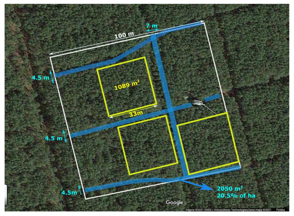
2.1. Site Description

This research was conducted at the eddy covariance (EC) study site established in May 2018 near Mezyk (ME) village in north-western Poland (52°50’ N, 16°15′ E). The forest was planted after a fire in 1992. It is an even-aged monoculture dominated by Scots pine (Pinus sylvestris L.) with approximately 1% admixture of silver birch (Betula pendula Roth).
In order to identify the stand structure at the study area, three square experimental plots were established, each with an area of approximately 1089 m2 (33 × 33 m) (Figure 1). The number of trees (Scots pine) was counted at each plot, and tree DBH was measured. The sum from all three plots was extrapolated to obtain the total number of trees per 1 ha, considering the contribution of roads, free spaces and birch plantations. The stand density was estimated to be 4262 trees ha−1. The average tree height in this area was 10.49 m (standard deviationof 0.99 m; median distribution = 10.15 m) [25]. The average diameter at breast height (DBH) was 9.5 cm. Based on three soil pedons, the soil type was determined to be Brunic Arenosoil.

2.2. Eddy Covariance and Meteorological Measurements

The EC system was composed of an open-path analyzer (IRGA, model LI-7500DS, LI-COR Inc., Nebraska, NE, USA) combined with a three-dimensional (3D) anemometer (model WindMaster Pro, Gill Instruments, Hampshire, UK) and smart flux systems. This was installed at the top of a 22 m-high flux tower, to measure the fluxes of trace gases (CO2 and H2O) exchange with the atmosphere. These measurements have been carried out since May 2018. Basic meteorological factors were continuously recorded, including four components of the surface radiation balance (model CNR4 Kipp&Zonen Niderland, Delf, Netherlands), air temperature (Ta) and air humidity measured at the top of the tower and at 2 m above the ground (Rotronik, Bassersdorf, Germany), as well as bulk precipitation (P)-tipping bucket rain gauge (model 52202-L, R. M. Young Company, Michigan, MI, USA). Soil temperature and soil water content (SWC) were measured at a depth of 2 cm in mineral soil (under the organic layer) using TDT Soil Moisture (SDI-12) sensors (Acclima, Meridian, Idaho, USA) with five replicates. In addition, the soil temperature was measured at five different profiles randomly placed around the EC tower, each at 2 and 5 cm deep. Since there were gaps in the P records collected here, continuous P measurements were obtained from the Miały rainfall station of the Institute of Meteorology and Water Management (IMiGW) network, located 2 km from ME. Daily observations were used instead of in situ measurements for the whole study period.

2.3. Dendrometer Measurements and Tree Circumference Increment Calculations

Within the main research area (white square, Figure 1), five groups of five Scots pine trees were chosen for continuous dendrometric measurements. A band dendrometer (model DR26E dendrometric increase sensors, EMS Brno, Brno Czech Republic) was installed at the breast height (130 cm from the soil surface) of each of these 25 selected trees. The recorded circumference increment data was sent to the datalogger (Datalogger GreyBox N2N, EMS Brno, Brno, Czech Republic) at a frequency of two minutes, and averaged to half-hourly values, corresponding to a measurement resolution of 0.002 m. The so-called “average tree” growth within the studied ecosystem was obtained by averaging DBH increments from all 25 dendrometers. Dendrometric phases were then determined based on the course of DBH increment within the entire investigation period. The beginning of wood growth in a particular year was set as the end of the growth phase in the previous year, considering the maximum winter contraction. Calculations and data analyses were performed with R software (R version 4.0.2, The R Foundation for Statistical Computing) [26].

2.4. Biomass Inventory of the Individual Parts of the Model Trees

The biomass of five sample trees was determined by an inventory carried out at the turn of spring and summer 2018 [25]. For this purpose, a sample area of 0.03 ha was established. Of the 114 trees within this area, five model trees were selected and extracted. Their DBH represented the average values for the main research plot (Table 1). The DBH measurement was made by the forest cluster. Sectional measurements were taken on approximately 1 m sections of the tree trunk (Figure 2). The stem was then pruned, and the separated branches were divided into two categories: main branches, and fine branches with needles. The root system was also excavated for each of these five model trees. The main roots (at least 2 mm thick) were cleaned and the trunks were collected.
The contribution of components such as deadwood (above and below ground) and undergrowth in the total stand biomass was estimated separately at four sample areas (50 m2 each). Two smaller circular areas (approximately 0.2 m2) were set up within these areas (established by tossing a hula hoop), and a single sampling was performed by collecting plants from these small areas. All herbaceous plants, bryophytes, and woody plants up to 0.5 m high were collected and cut at the ground with shears. Samples of fine roots were collected from the center of each area using a cylindrical root collector (volume 1387 cm3, diameter 4.7 cm, height 20 cm) inserted to a depth of 0–20 cm and 20–40 cm. Dead aboveground wood biomass consisted of standing deadwood, living and dead thick branches (>7 cm in diameter at the thicker end). For the belowground dead wood estimation, stems or trunks of torn, broken and felled trees were included. Dry mass was also determined for each tree separately by drying individual tree parts at 65 °C. The results of biomass estimations of the five model trees are presented in Table 1. Carbon content in the dry biomass was calculated as the average of the samples from the trees’ components. The highest value was characteristic for stem and bark, and the lowest for fine roots, resulting in an average of 50% carbon content in dry biomass. NPP was calculated as 50% of the total dry biomass. Within the main study area (1 ha), other forest ecosystem elements such as deadwood (both above and below ground) and undergrowth (herbaceous plants, bryophytes, woody plants up to 0.5 m high) constituted approximately 6.3% of the total dry biomass.

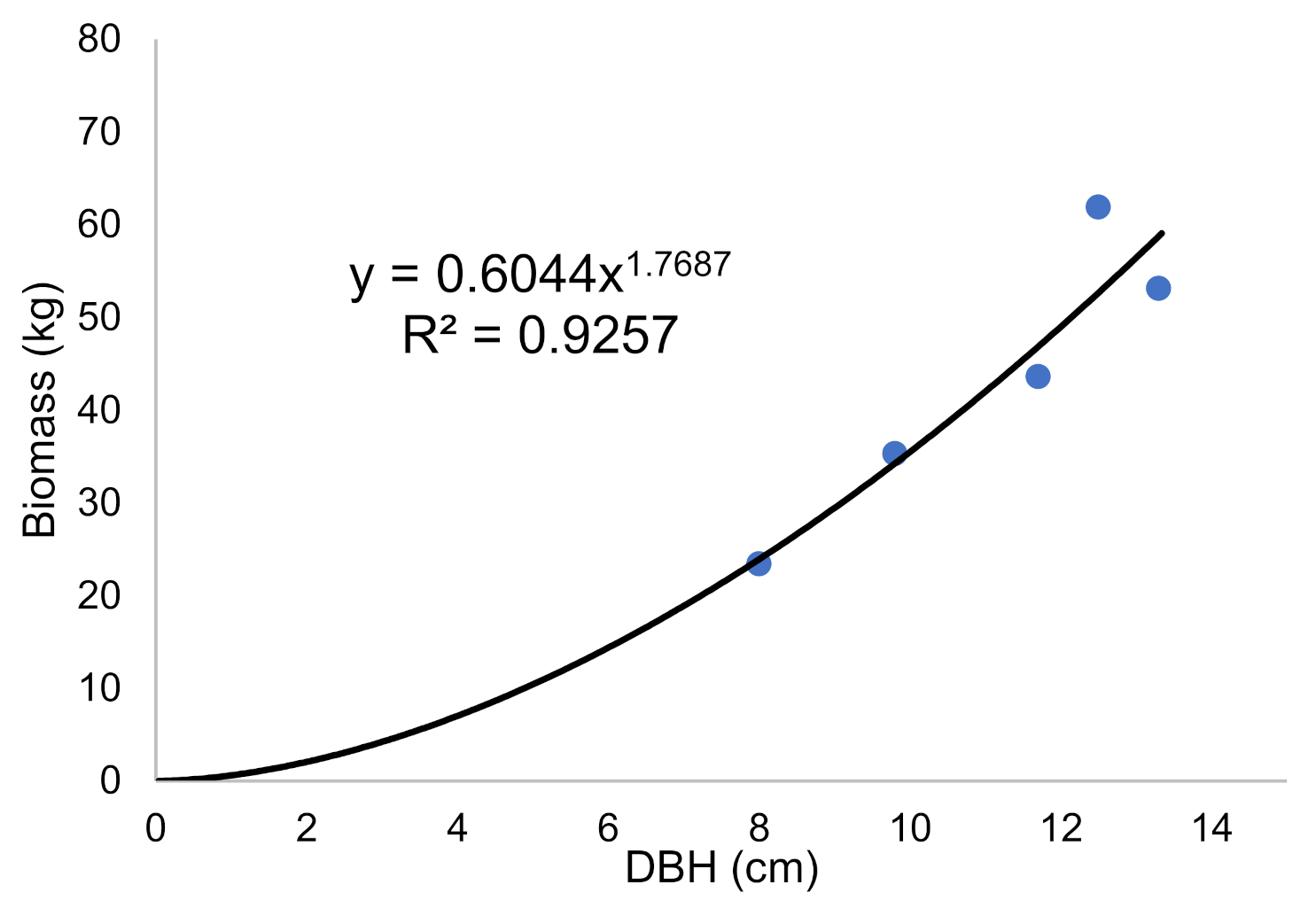
2.5. In Situ Allometric Equations—The Relationship between Biomass of Tree Components and Their DBH

The total dry biomass of individual trees was correlated with their DBH in order to obtain site-specific allometric equations (Figure 3). Fitted non-linear regression parameters suggest that total dry biomass is highly correlated with DBH–the coefficient of determination exceeded 0.9. A power-type regression was used, since this function type best fits the data. The approach of relating total biomass of the tree to its DBH will hereinafter be referred to as the “site-specific method M1”.
To estimate the biomass of the different tree components, particular functions can be fitted. However, Picard et al. (2012) suggested that these should be used together (equation matrix) rather than separately (simple sum) when calculating total tree biomass [27]. In our work, the parameters were obtained for individual components based on direct in situ measurements; these were summed to derive the whole tree biomass. Stem increment of the average tree determined from dendrometer measurements was used to relate the biomass of individual tree components to DBH. The resulting set of empirical equations is presented below (Equation (1)), hereinafter referred to as the “site-specific method M2”.
T o t a l   d r y   b i o m a s s = 0.3932   D B H 1.7298 a                                           R 2 = 0.99 0.0122   D B H 2.5525 b                                           R 2 = 0.72 0.0586   D B H 1.635       c                                             R 2 = 0.75 0.0537   D B H 1.5844   d                                             R 2 = 0.70   0.0381   D B H   2.0549 e                                           R 2 = 0.87 0.014   D B H + 0.8245 f                               R 2 = 0.67
where DBH—diameter at breast height, a—stem + bark biomass, b—thick branches biomass, c—needles biomass, d—thick roots biomass, f—small roots biomass. The coefficient of determination (R2) for the obtained equations is given in square brackets.
In addition, we compared the results obtained from in situ allometric equations with those from Wegiel and Polowy [1], which were determined to be decent empirical estimations for comparison. Their research area was located about 50 km northwest of the Mezyk site, and their equations were derived for 82-year-old Scots pine. The climatic and meteorological conditions of both ecosystems are very similar.

2.6. Eddy Covariance Data Processing

Raw net ecosystem exchange (NEE) fluxes were calculated using commercial EddyPro software (version 7.0.1, Lincoln, NE, USA) with default settings. According to this mode, several processing steps were applied: despiking, amplitude resolution, drop-outs, absolute limits, skewness and kurtosis, discontinuities analysis. The following corrections were then made: angle of attack, since a Gill anemometer was used, double rotation correction, the time delay due to the separation of measuring instruments, block averaging and density correction (WPL). Basic filtering included stationarity test according to Mauder and Foken, [28], and thus only data with “0” flag were used here for further computation. Fluxes measured during low turbulent conditions were removed by using friction velocity threshold as a sufficient turbulence parameter [29,30,31]. For this purpose, the measurement period was arbitrarily divided into monthly sub-periods. Friction velocity threshold (u*th) was calculated for each month and the data was filtered in these periods according to the given u*th value. Outliers were then removed, assuming monthly integration periods and two standard deviations value as a criterion. The “anomalize” package for R was used for this purpose [32]. The rate of concentration change (i.e., the storage flux) of CO2 and H2O (ΔSCO2 and ΔSH2O, respectively) in the air column below the EC system was also calculated in the EddyPro software [33]. Briefly, storage fluxes are obtained as the difference between the average concentration in the beginning and in the end of a specific averaging period (most often 30 min, as also in our study). This yielded similar results to those obtained with the concentration profile approach [34]. Both ΔSCO2 and ΔSH2O values were accounted for in the final fluxes calculations [35]. Finally, NEE fluxes gap-filling and partitioning into GPP and ecosystem respiration (Reco) was performed using the “REddyProc” package [30] in the R environment [26], following the Reichstein night-time approach of using the air temperature measured under a canopy at 2 m above ground for the Reco fluxes estimation [31,36,37,38,39]. In addition, water fluxes (given as evapotranspiration, ET) obtained by the EC method were calculated and gap-filled according to the same methodology as for the carbon fluxes, also using the REddyProc package [30].
The assimilation of atmospheric CO2 is undoubtedly correlated with wood growth. However, due to the complexity of distinguishing irreversible seasonal wood growth from the increase in tree volume that results from reversible swelling and contraction of the stem, it was very difficult to determine this relationship, especially over a period of less than one year. The occurrence of the periodic reversible shrinkage or expansion of DBH mainly resulted from changes in the water content of plant tissue, and not from the actual increase in biomass. Nevertheless, there are various concepts regarding tree growth during periods of reversible contraction in response to water stress conditions. One such example is a concept of “zero growth” during periods of stem shrinkage, which utilizes a water-related growth threshold [40]. During a dry period, the stem may increase in size as a result of water-related swelling of stem tissues [41,42]. For example, a slight increase after longer periods of water shortage was observed in two deciduous and two evergreen trees species in one dry and two wetter sites in Switzerland; this increase was interpreted as activity during periods of stem swelling and shrinkage [40]. Therefore, due to these difficulties, we have presented the annual stem increment and the total biomass growth for both years.

2.7. Carbon Use Efficiency (CUE) and Definition of Vegetation Period

CUE (CUE = NPP/GPP) was calculated using the results obtained both by biometric and EC measurements. GPP obtained from the EC system has been summarized for each study year starting from the point when the annual cumulative value of net ecosystem productivity (NEP) was no longer negative relative to the maximum value of the previous year. The end of this range was defined when the positive annual growth of NEP ended and the cumulative values began to decline, suggesting the overall advantage of emissions over CO2 absorption. This period will be referred hereinafter to the “vegetation period”, in order to differentiate this from the wood growth period (B) when the carbon absorbed during photosynthesis was turned into the growth of tree biomass.
For clarity, all described calculations and the final combination of results from dendrometric, biometric and EC measurements are presented in the diagram below (Figure 4).

2.8. Drought Conditions Estimates

To present the characteristics of individual months in terms of drought occurrence over the study period (2019–2020), the SPEI Global Drought Monitor database was used [43]. Standardized precipitation evapotranspiration index (SPEI) is a multiscale drought index that combines precipitation and temperature data based on normalization of water balance estimation [44]. Detailed methodology for calculating and applying this indicator is presented in the literature [44,45,46]. In addition, complete description of the used data and metadata can be found online [https://spei.csic.es/home.html access on 1 February 2021].

3. Results

3.1. Drought Occurrence Detected by SPEI Index Monitoring

SPEI index values over a three-month time scale were used here, since it is assumed that such scale allows effective assessment of meteorological drought intensity. The reference period ranges from 1950 to 2020, and the values of this index since 1981 are shown in Figure 5. Lower negative results indicate more severe drought in a given month. Extreme droughts are characterized by SPEI values of less than −2. Such conditions occurred at ME study area in August 2019, as well as in July and August 2018. It should be noted that even though there were several dry months during both study years, fewer severe drought events occurred in 2020 than in 2019 (Figure 5).

3.2. Meteorological Conditions and CO2 and H2O Fluxes Courses

The highest monthly precipitation for 2019 was recorded in September (more than 100 mm), and the lowest in April and June (both less than 20 mm). In 2020, the drought conditions in April were even more severe, as the sum of P for that month did not exceed 10 mm. On the other hand, precipitation conditions during the summer season of 2020—which is important for tree growth and development—were generally much more favorable than in the previous year (Table 2). In 2020, the highest monthly precipitation total was recorded in July, and amounted to slightly less than 100 mm. In general, 2019 was drier and warmer than 2020. However, annual GPP totals were quite similar, while ET reached significantly higher values in 2020, particularly during the summer (Table 2). The ratio between annual totals of Reco and GPP were similar between the years (0.75 and 0.76 in 2019 and 2020, respectively). Thus, the difference between GPP and Reco, which in principle constitutes net primary productivity (NEP), was only slightly higher in 2019. Compared to 2019, 2020 was characterized by lower mean Tair, vapor pressure deficit VPD, global radiation (Rg), and higher mean SWC. Aside from spring, higher Reco totals were measured in 2020 on the seasonal scale. ET sums for spring and summer, as well as annually, were also higher in 2020 than the previous year. Even though ET totals in autumn were almost equal in both years, precipitation totals were substantially higher in autumn of 2019 than in 2020 (Table 2). In spite of the higher Tair, VPD and Rg in autumn 2020, the SWC was almost the same as in 2019. Regardless of the season, GPP totals were higher with higher average Tair and higher SWC. Even though increased precipitation was recorded in spring and autumn of 2019, this did not correspond to increasing SWC. As such, SWC in spring of 2019 was lower than in 2020. It should be noted that in spring and summer (i.e., the most important periods for plant growth), photosynthesis rates (GPP) were higher in 2019. This likely resulted from the higher average temperatures and slightly higher radiation that summer, even with lower soil water content (Table 2).

3.3. Identification of Specific Periods during Wood Growth

In order to determine the individual dendrometric phases, the stem increment for both studied years was followed. In order to distinguish growth processes from reversible water-related processes and to avoid the disturbing effects of rapid freezing-induced changes in stem diameter during winter, the starting point for annual radial growth of the stem was set as the previous year’s culmination [47]. The point of the maximum winter contraction (MWC) occurred at a similar time in both years (21 April 2019 and 23 April 2020) (Figure 6a). From that moment, rapid relaxation began and DBH increased simultaneously. However, in order to quantify the actual increase, the biomass growth was estimated from the beginning of seasonal growth after rehydration—i.e., 1 May and 2 May for 2019 and 2020, respectively, until the end of the growing period when DBH stopped increasing. In early October 2019, the end of the seasonal increase in biomass was recorded (tree circumferential growth), while the DBH growth continued in 2020 until mid-October (Figure 6a). Thus, the total period of actual wood growth (B) was 14 days longer in the second year. During winter, the change in DBH was caused by reversible trunk variations. The beginning of the seasonal biomass growth was then assessed from the cessation of growth in the previous year (P0 point). By applying the methodology described in the Materials and Methods section (Figure 4) and recognizing B period range for the average tree, NPP was calculated for both years. (Figure 6b).
Differences in the course of DBH growth between the years are visible, especially in summer—August in particular—when dry conditions prevailed in 2019 year (Figure 6a). According to the theory of zero growth during periods of stem shrinkage, the increase in biomass was significantly limited in the most optimal period in terms of productivity [40], since any potential growth-induced expansion is associated with the time after tree water deficit-induced reversible stem shrinkage has completely ceased. In 2019, the increase in DBH was on average 0.14 mm per tree, while in 2020 it was 0.16 mm, so the difference was over two hundredths of a millimeter. Nevertheless, considering there is over 4200 trees per hectare in our study area, even a small change in DBH increment over a year can translate into an increase in carbon accumulation in the biomass by as much as 0.6 tons per hectare (Figure 6; Table 3).

3.4. Stand Biomass and CUE Estimations

As shown above, the total increase in biomass was determined starting from the point after the rehydration period (Figure 6a). EC-derived GPP for the vegetation period ranged from the beginning of March to the end of September for both years (Figure 6b.). The estimates of NPP and GPP allowed the calculation of the CUE values. It should be pointed out that GPP summarized for the vegetation period represents the total CO2 amount absorbed from the atmosphere which could be then potentially be built into the tree’s tissues as carbon (C).
Using the first method of the allometric equation with the general formula (M1), an absolute increase in dry biomass of 0.9 kg per average tree was estimated in 2019, and 1.2 kg in 2020 (Table 3). Considering the number of trees estimated at our study site (4262 per hectare), the total increase in dry biomass was approximately 4.3/4.4 t C ha−1 in 2019, and 5.5/5.7 t C ha−1 in 2020 (calculated by M1/M2 method, respectively). Consequently, NPP was approximately 2.1/2.2 t C ha−1 in 2019, and 2.7/2.8 t C ha−1 in 2020. A possible uncertainty was also given, considering an error that could occur when determining the phases of the biomass increase (±0.01cm for initial increment measurement; Table 3). This also reveals how the 0.01 cm of the average DBH increment for each tree translates into the estimation of the total forest biomass during the year (the difference of 0.01 mm, depending on the method, gives an error of ca. 0.3 kg of the total dry biomass of the stand unit area).
The total amount of absorbed CO2 (GPP) during the vegetation period was higher in 2019 than in 2020 (Table 3). However, the sum of respired CO2 (Reco) during the same period was slightly higher in 2020 (10 t C ha−1) than in 2019 (9.7 t C ha−1). Hence, the difference between GPP and Reco, which essentially constitute Net Ecosystem Productivity (NEP), was higher in 2019. Nevertheless, CUE, which is a key indicator of how much absorbed CO2 was fixed and converted into fresh wood growth, was higher in 2020. CUE has been calculated both for the vegetation period (different periods for total annual NPP and total annual GPP) and the wood growth period (B) (Figure 6; Table 3). It was found that CUE for the vegetation period remained fairly low in both years, although it was higher in 2020; depending on the method, it was estimated to be 0.19/0.20 (M1/M2). In 2019, it was estimated to be 0.15 using both methods. For the B period, CUE values were 0.18/0.19 and 0.23/0.24 in 2019 and 2020, respectively (Table 3).

4. Discussion

4.1. NPP Biometric Estimates

Forests absorb carbon dioxide in the process of photosynthesis. Part of it is fixed in plant biomass (carbon sequestration), while some returns back to the atmosphere through ecosystem respiration. In this study, biometric measurements and derived site-specific allometric equations (M1/M2 method) showed that, on average, 2.0/2.1 t C ha−1 was sequestered in wood tissues of a 25-year-old Scots pine stand (annual NPP totals) in dry 2019. In the following year, characterized by moderate water availability, these values were 2.6/2.7 t C ha−1 (Table 3). Among various forest types, boreal forests are the least productive (the lowest annual NPP totals) in comparison to temperate and especially tropical forests. The results from the global studies conducted by Xu et al. suggest that, on average, less than 10 tons of carbon per hectare is assimilated in boreal forests in the form of new woody tissue, while more than 12 tons of carbon per hectare is sequestered in temperate forest ecosystems [48]. On the other hand, Xu et al. [48] have shown that across biomes, the highest NPP is found in middle-aged forests (mean = 6.5 t C ha−1), while young forests showed the lowest NPP (average = approx. 4 t C ha−1) [48]. The respective results presented in our study indicate annual NPP totals several times lower than the average for boreal forests, and roughly two times lower than the average for young forests, even though the research was conducted at a Scots pine stand located in a temperate climatic zone. This surprising outcome is likely related to the young age of the stand, and further to the extreme meteorological conditions that occurred in the year 2019 (extreme drought) and slow recovery in 2020, in which the impact of the previous year’s conditions was still noticeable. Another reason for these lower values could be the differences in methodology between cited study presented above, which covers various species of the climatic zones, while our study concerns only one dominant tree species. Drake et al. [17] reported NPP values twice as high as those found at the ME site—roughly 4 t C ha−1 year−1 for forests of loblolly pine older than 20 years. These authors also report the highest NPP for trees younger than 20 years (assuming NPP as the sum of wood, foliar, and fine roots production), concluding that for this pine species, NPP generally decreases with age after reaching this maximum [17]. There has been broad discussion in the literature addressing the question of the decrease in NPP with forest age. This revealed, inter alia, that the decline in GPP—rather than an increase in Ra—was the cause of NPP decrease as pine trees aged [17]. Sapwood respiration, which is an important component of Ra, also decreases with age. The decrease in pine GPP was driven by the age-related decrease in canopy conductance, which is in line with the hydraulic limitation hypothesis of Ryan et al. [17,49]. Hence, it is expected that in the future, stand biomass growth that was currently estimated for the Mezyk site will most probably decrease. Further studies are needed to show at what age exactly NPP reaches its maximum for this temperate Scots pine stand, and what meteorological conditions will be conducive to this.

4.2. Differences between Meteorological Conditions in 2019 and 2020 and Their Impact on NPP and GPP, and CUE Values

It has been suggested that carbon use efficiency decreases with forest age [19]. In our study, CUE increased in 2020 compared to the previous year, which comes from only slightly higher annual total of GPP with generally higher NPP. This can be explained by more favorable environmental conditions—higher average soil water content and higher precipitation totals, both annually and in the summer—which led not only to a higher NPP/GPP ratio, but also to higher total ET fluxes. Stomata minimize the amount of transpired water per given gross primary productivity (GPP) rate under scarce water conditions, which has a theoretical basis in photosynthesis and air humidity control on stomatal conductance [50]. Therefore, by reducing water loss during drought conditions while maintaining photosynthesis at a fairly stable level for as long as possible, drought conditions have a greater impact on the annual variation in ET totals than GPP. ET sums were lower both in spring and summer of 2019 (Table 3.), when dry conditions were more severe. The differences in meteorological conditions between 2019 and 2020 resulted in only slight changes in photosynthesis and transpiration fluxes. Considering their influence on NPP, the impact was significant—almost 1 t C ha−1 more in woody biomass in 2020 compared to dry 2019. The drought that occurred in 2019, especially in June and August, has particularly important consequences. Since the highest GPP values were observed in summer months (in 2020 constituting 52.8% of the total vegetation period GPP, and 44.3% of its annual total), their contribution was crucial on the annual basis. Thus, significant reduction due to drought can lead to the decrease in summer contribution to both vegetation period and annual GPP totals. Nevertheless, in 2019, especially with a very dry August, the share of GPP in relation to the entire year and the vegetation period was not less than in 2020 (52.8% and 45%, respectively).
The average annual CUE from across a range of forest ecosystems has been estimated as approximately 0.5, which means that, on average, half of the carbon absorbed in the photosynthesis process is allocated to the growth of wood tissue [51,52,53]. Nevertheless, reported CUE ranges from 0.2 to 0.8 depending on species, environmental, age and methodology [19,51,53,54]. According to the study of different-aged pine stands (6-, 19-, 34-, and 69-years-old) in southern Ontario, Canada, CUE varies greatly with age. Annual mean CUE during 2005–2008 amounted to 0.61, 0.33, 0.50, 0.43, respectively [2]. This research considered different climatic conditions of a 30-year norm, where the year 2005 was identified as hot and dry, 2006 as hot and wet, 2007 as warm and dry, and 2008 as a nearly average year. In another study conducted in a managed forest (afforestation) with predominantly Pinus halepensis species (Yatir Forest, Israel), annual CUE ranged from 0.38 to 0.42, depending on the method used [51]. Thus, it can be conluced that in relation to similar ecosystem types (temperate pine forest), the CUE values presented in our study are quite low.
It is worth emphasizing that wood growth is even more drought sensitive than photosynthesis itself [24,55,56]. Nevertheless, when severe drought occurs, the photosynthesis rate slows due to stomata enclosure, and biomass growth is also reduced [57]. In the research by Campioli et al. conducted at a temperate beech forest, it was shown that annual GPP totals were significantly lower in years when drought occurred, compared to wetter years; a corresponding significant decrease in NPP was also seen [24]. Hence, in dry years the annual NPP/GPP ratio was still quite high (40–44%). The data shows that the reduction in annual net primary productivity in our study is related to the occurrence of conditions distant from the comfort zone (in this case, the occurrence of drought). This can be explained by the adaptation process in which forest ecosystems adjust their optimal productivity to the climatic conditions of the region that used to be close to the average [2]. In addition, Peichl et al. [2] observed a negative relationship betwen NPP and air temperature, which is opposite to the common understanding of the NPP climate response in forests [58]. Such effect also seems true for our research, where a lower NPP total occurred in the warmer year. However, this was more likely caused by drought and/or heat stress, which are generally limiting conditions of NPP in warmer years [59]. Importantly, our results are based on only two years of data (one of which being extreme climate conditions), making them less reliable in supporting the findings of Peichl et al. [2]. Moreover, summer of 2020 was cooler, such that the total GPP sum was lower than in the previous year. A higher total NPP is recorder in years characterized by dry conditions—for example in the research by Campoli et al., who found a relatively high NPP during the extremely dry 2003, which is even more difficult to explain [24]. One possibility is interannual growth buffers such as C reserves and buds preformed in the previous year, especially if it was climatically medium or wet. This was not the case in our study, since 2019 followed a very dry year, which probably also influenced the presented biomass growth results. The average value of the SPEI index from March to October in 2018 amounted to −1.64. Extreme drought was evident in June (SPEI = −2.36) and August (SPEI = −2.09). Furthermore, extreme conditions such as drought often hinder thorough analysis and interpretation, as well as different physiological responses of plants to the existing conditions. Plants adopt a special “strategy” as they partition resources among different organs for optimal functioning. This helps to maximize life span, seed production, and growth rate under particular environmental conditions [60]. It was found that in a tropical forest, the lowest CUE (0.35) occurred in undisturbed forest patches, while slight forest disturbance had a positive effect on CUE increase (0.62) [7]. Moreover, the authors of this study suggest that monocultures had a higher CUE than mixed forest stands. In our research, the difference in NPP resulted in approximately 0.600 t C ha−1. Applying the literature-derived method (excluding dead branches) yielded in 0.566 t C ha−1 for the ME site [1]. The literature-derived absolute sums of biomass and NPP were approximately 20–30% lower than those calculated by constructing equations based on in situ data, which amounted to 1.7 C ha−1 for 2019 and 1.9 C ha−1 for 2020. It was thus concluded that in biomass research, site-specific equations are more likely to give robust results. The literature-based solution resulted in very low CUE, which amounted to roughly 0.13 for 2019 and 0.15 for 2020.

4.3. Difficulties in Calculating NPP as a Part of GPP Using Different Approaches

The use of allometric relationships between stem diameter (DBH) and tree biomass can lead to systematic errors in aboveground NPP estimates [14]. It has also been suggested that the use of inadequate allometric equations and uncertainty in the estimates of fine-grained litter production potentially introduces significant errors in biometric estimates of NPP [2,61,62,63]. Several reports have showed that discrepancies between biometric and EC measurements on an annual basis may be caused by the time-lag between carbon assimilated in photosynthesis and its allocation represented by stem growth [64]. Nevertheless, relative annual changes of NEP were found to be comparable between the two estimation methods, even when there were differences in its absolute values [65,66,67]. In our research, lower productivity in spring and summer (GPP) was associated with less severe drought events in 2020, although Reco increased in the summer and autumn of this year and was thus higher than in 2019. In general, the highest respiration fluxes were found to be in the summer, apparently caused not only by high temperatures but also higher overall plant activity (leaves and fine-roots are present and active, growth is occurring, etc.) [31]. The total EC-derived sum of NEP from March to October was higher in 2019 by 0.5 t C ha−1 than in 2020 (Table 3). Higher NPP values were estimated for the same period in 2020 with biometric methods. Thus, the results obtained in our study suggest that higher NPP values estimated with biometric equations are associated with lower GPP and higher CUE. These may occur together with a lower NEP derived from EC measurements in the same season (Table 3). Notably, it is assumed that if the share of GPP used for respiration changes depending on soil conditions, NPP should also vary according to the ratio of NPP to GPP. Collati and Prentice attempted to answer the question posed by Waring et al. [52] 20 years earlier, and investigated if NPP of forests is a constant fraction of GPP. Their results provided evidence to reject the hypothesis of a universal or constant ratio of NPP to GPP, which in fact changes under disturbances, ageing and changes in biomass accumulation with changing climate, soil fertility and management practices. These have all been indicated to influence the ratio of NPP to GPP, likely in a non-mutually exclusive manner [68]. However, this approach was already implemented as a simplified concept in a large number of ecosystem models. In our research, such variation was also true: very similar GPP values estimated for different years under varying conditions did not change proportionally to NPP totals in the studied period. On the contrary, they indicated greater wood growth in a moderately wet year with higher soil water content during spring and summer.
It is often considered that low CUE results do not reflect a significant underestimation of NPP, but are more likely related to the overestimation of GPP, since CO2 fluxes measured by the EC method are prone to uncertainties. Different conclusions have been reached when using the open path (OP) analyzers as compared to closed path (CP) analizers. For instance, Richardson et al. compared random CO2 fluxes using concurrent CP and OP measurements above soybean and maize crop [69]. The authors found differences in random flux uncertainty to be negligible during the day, while at night the random uncertainty of the OP system exceeded that of the CP systems by up to 20%. On the contrary, another study suggested very small differences in the random flux uncertainty between CP and OP systems [70]. Some of the latest results from Bog Lake Peatland flux tower (US-MBP on AMERIFLUX) suggest that during the growing season, the OP system measured larger net daytime CO2 uptake than the CP sensor did, while the OP and CP CO2 fluxes tended to converge at night [71]. A specific difficulty in the methodology used here was the appropriate estimation of the end of period for the stem diameter increment in 2018, which was the reference point for the start of the biomass growth in 2019. Interpreting data from band dendrometers becomes difficult due to reverse contractions and swelling of the stem, especially in winter. It has been found that the effects of freezing temperatures on plant functions differ greatly from those caused by low, but non-freezing, temperatures [72]. Severe dehydration can be caused by the formation of extracellular ice under freezing conditions, so that the plant retains its ability to cope with these conditions [73]. As a consequence of hardening the plant in response to cold, the lipid composition [74], membrane structure [75] and sugar concentration [76] vary greatly, and some specific metabolites, including proteins that prevent freezing, accumulate [72,77]. This, among other issues, caused the visible swelling of the stem that was observed in January 2019, which was not related to wood growth.

5. Conclusions

Our study of a 25-year-old temperate Scots pine monoculture in north-western Poland has led to several conclusions:
Using five sampled trees at the Mezyk research area, the combination of biomass measurements, continuous dendrometric measurements, and recognition of the stand structure allowed site-specific allometric equations to be derived. Absolute values of wood biomass growth in 2019 and 2020 were also calculated, which were more robust than literature-derived equations.
The drought in spring and summer 2019 was preceded by even more severe drought in 2018. As a result of this extreme water conditions, the NPP in this young Scot pine monoculture was about 0.6 t C ha−1 lower than in moderately wet 2020.
The higher temperatures in spring and summer led to higher GPP in these seasons in 2019, despite the lower precipitation and soil water content. On an annual basis, GPP totals were comparable between the years. Slight changes in GPP sums during vegetation periods of the study period did not correspond to proportional variation in NPP total sums, which were considerably higher in the wetter year.
The thermal and humidity conditions that occurred in 2020 were more favorable than in 2019. This resulted in higher Reco and NPP sums, despite the lower GPP and NEP in 2020, which resulted in higher efficiency in the use of carbon assimilated due to photosynthesis for new wood production (CUE).

Author Contributions

Conceptualization: P.D. and K.Z.; methodology: P.D.; formal analysis: J.O., S.M., T.V., M.U.; resources: J.O., S.M.; data curation: P.D., M.U.; writing—original draft preparation: P.D.; writing—review and editing: K.Z., M.U., T.V.; visualization: P.D.; supervision: M.U.; project administration: J.O.; funding acquisition: J.O., S.M. All authors have read and agreed to the published version of the manuscript.

Funding

This research was supported by funding from General Directorate of the State Forests, Warsaw, Poland (project LAS, No OR-2717/27/11).

Data Availability Statement

Data available on request. The data presented in this study are available on request from the corresponding author. The data are not publicly available due to the unfinished repository, however, the authors are willing to share it.

Acknowledgments

We would like to express our gratitude to soil scientist team from the Department of Ecology and Silviculture, Faculty of Forestry, University of Agriculture in Krakow, for their fieldwork, expertise and preliminary data analysis, and to the Tyumen region government in accordance with the Program of the World-Class West Siberian Interregional Scientific and Educational Center (National Project “Nauka”). The authors would like to thank Jacquelin DeFaveri from Language Centre at University of Helsinki for their help with revising the language.

Conflicts of Interest

The authors declare no conflict of interest. The funders had no role in the design of the study, the collection, analyses, and interpretation of data, the writing of the manuscript, or in the decision to publish the results.

References

  1. Wegiel, A.; Polowy, K. Aboveground carbon content and storage in mature scots pine stands of different densities. Forests 2020, 11, 240. [Google Scholar] [CrossRef] [Green Version]
  2. Peichl, M.; Brodeur, J.J.; Khomik, M.; Arain, M.A. Biometric and eddy-covariance based estimates of carbon fluxes in an age-sequence of temperate pine forests. Agric. For. Meteorol. 2010, 150, 952–965. [Google Scholar] [CrossRef]
  3. Dixon, R.K.; Solomon, A.M.; Brown, S.; Houghton, R.A.; Trexier, M.C.; Wisniewski, J. Carbon Pools and Flux of Global Forest Ecosystems. Science 1994, 263, 185–190. [Google Scholar] [CrossRef]
  4. Denman, K.L.; Brasseur, G.; Chidthaisong, A.; Ciais, P.; Cox, P.M.; Dickinson, R.E.; Hauglustaine, D.; Heinze, C.; Holland, E.; Jacob, D.; et al. Couplings Between Changes in the Climate System and Biogeochemistry. In Climate Change 2007: The Physical Science Basis. Contribution of Working Group I to the Fourth Assessment Report of the Intergovernmental Panel on Climate Change; Solomon, S., Qin, D., Manning, M., Chen, Z., Marquis, M., Averyt, K.B., Tignor, M., Miller, H.L., Eds.; Cambridge University Press: Cambridge, UK; New York, NY, USA, 2007; pp. 501–568. [Google Scholar]
  5. Urban, J.; Čermák, J.; Ceulemans, R. Above- and below-ground biomass, surface and volume, and stored water in a mature Scots pine stand. Eur. J. For. Res. 2015, 134, 61–74. [Google Scholar] [CrossRef] [Green Version]
  6. Manickam, V.; Krishna, I.V.M.; Shanti, S.K.; Radhika, R.; Campus, B.V.; Pradesh, A. Biomass Calculations for Carbon Sequestration in Forest Ecosystem. J. Energy Chem. Eng. 2014, 2, 30–38. [Google Scholar]
  7. Kunert, N.; El-Madany, T.S.; Aparecido, L.M.T.; Wolf, S.; Potvin, C. Understanding the controls over forest carbon use efficiency on small spatial scales: Effects of forest disturbance and tree diversity. Agric. For. Meteorol. 2019, 269–270, 136–144. [Google Scholar] [CrossRef]
  8. Juráň, S.; Grace, J.; Urban, O. Temporal Changes in Ozone Concentrations and Their Impact on Vegetation. Atmosphere 2021, 12, 82. [Google Scholar] [CrossRef]
  9. Bréda, N.; Huc, R.; Granier, A.; Dreyer, E. Temperate forest trees and stands under severe drought: A review of ecophysiological responses, adaptation processes and long-term consequences. Ann. For. Sci. 2006, 63, 625–644. [Google Scholar] [CrossRef] [Green Version]
  10. Kumar, A.; Kumar, M. Estimation of Biomass and Soil Carbon Stock in the Hydroelectric Catchment of India and its Implementation to Climate Change. J. Sustain. For. 2020, 39, 1–16. [Google Scholar] [CrossRef]
  11. Rai, P.; Vineeta; Shukla, G.; Manohar K, A.; Bhat, J.A.; Kumar, A.; Kumar, M.; Cabral-Pinto, M.; Chakravarty, S. Carbon storage of single tree and mixed tree dominant species stands in a reserve forest—Case study of the eastern sub-himalayan region of india. Land 2021, 10, 435. [Google Scholar] [CrossRef]
  12. Zianis, D.; Muukkonen, P.; Mäkipää, R.; Mencuccini, M. Biomass and Stem Volume Equations for Tree Species in Europe; The Finnish Society of Forest Science: Helsinki, Finland; The Finnish Forest Research Institute: Helsinki, Finland, 2005; Volume 4, ISBN 9514019830. [Google Scholar]
  13. Wohlfahrt, G.; Gu, L. The many meanings of gross photosynthesis and their implication for photosynthesis research from leaf to globe. Plant Cell Environ. 2015, 38, 2500–2507. [Google Scholar] [CrossRef] [PubMed] [Green Version]
  14. Chambers, J.Q.; dos Santos, J.; Ribeiro, R.; Higuchi, N. Tree damage, allometric relationships, and aboveground net primary production in a tropical forest. For. Ecol. Manag. 2001, 152, 73–84. [Google Scholar] [CrossRef]
  15. Chapin, F.S.; Woodwell, G.M.; Randerson, J.T.; Rastetter, E.B.; Lovett, G.M.; Baldocchi, D.D.; Clark, D.A.; Harmon, M.E.; Schimel, D.S.; Valentini, R.; et al. Reconciling carbon-cycle concepts, terminology, and methods. Ecosystems 2006, 9, 1041–1050. [Google Scholar] [CrossRef] [Green Version]
  16. Clark, D.A.; Brown, S.; Kicklighter, D.W.; Chambers, J.Q.; Thomlinson, J.R.; Ni, J. Measuring net primary production in forests: Concepts and field methods. Ecol. Appl. 2001, 11, 356–370. [Google Scholar] [CrossRef]
  17. Drake, J.E.; Davis, S.C.; Raetz, L.M.; Delucia, E.H. Mechanisms of age-related changes in forest production: The influence of physiological and successional changes. Glob. Chang. Biol. 2011, 17, 1522–1535. [Google Scholar] [CrossRef]
  18. Bruchwald, A. New Empirical Formulae for Determi- nation of Volume of Scots Pine Stands. Folia For. Pol. Ser. 1996, A 38, 5–10. [Google Scholar]
  19. DeLucia, E.H.; Drake, J.E.; Thomas, R.B.; Gonzalez-Meler, M. Forest carbon use efficiency: Is respiration a constant fraction of gross primary production? Glob. Chang. Biol. 2007, 13, 1157–1167. [Google Scholar] [CrossRef] [Green Version]
  20. Zanotelli, D.; Montagnani, L.; Manca, G.; Tagliavini, M. Net primary productivity, allocation pattern and carbon use efficiency in an apple orchard assessed by integrating eddy covariance, biometric and continuous soil chamber measurements. Biogeosciences 2013, 10, 3089–3108. [Google Scholar] [CrossRef] [Green Version]
  21. Law, B.E.; Sun, O.J.; Campbell, J.; Van Tuyl, S.; Thornton, P.E. Changes in carbon storage and fluxes in a chronosequence of ponderosa pine. Glob. Chang. Biol. 2003, 9, 510–524. [Google Scholar] [CrossRef]
  22. Doughty, C.E.; Goldsmith, G.R.; Raab, N.; Girardin, C.A.J.; Farfan-Amezquita, F.; Huaraca-Huasco, W.; Silva-Espejo, J.E.; Araujo-Murakami, A.; da Costa, A.C.L.; Rocha, W.; et al. What controls variation in carbon use efficiency among Amazonian tropical forests? Biotropica 2018, 50, 16–25. [Google Scholar] [CrossRef] [Green Version]
  23. Anić, M.; Ostrogović Sever, M.Z.; Alberti, G.; Balenović, I.; Paladinić, E.; Peressotti, A.; Tijan, G.; Večenaj, Ž.; Vuletić, D.; Marjanović, H. Eddy covariance vs. biometric based estimates of net primary productivity of Pedunculate Oak (Quercus robur L.) forest in Croatia during ten years. Forests 2018, 9, 764. [Google Scholar] [CrossRef] [Green Version]
  24. Campioli, M.; Gielen, B.; Göckede, M.; Papale, D.; Bouriaud, O.; Granier, A. Temporal variability of the NPP-GPP ratio at seasonal and interannual time scales in a temperate beech forest. Biogeosciences 2011, 8, 2481–2492. [Google Scholar] [CrossRef] [Green Version]
  25. Małek, S.; Pająk, M.; Wosś, B.; Jasik, M. Zapas węgla w biomasie drzewostanów sosnowych o różnym wieku wokół stacji pomiarowych: Tuczno, Mezyk, Tlen1 i Tlen2. In Rola Lasu w Pochłanianiu Dwutlenku Węgla z Atmosfery; Olejnik, J., Małek, S., Eds.; Wydawnictwo Uniwersytetu Przyrodniczego w Poznaniu: Poznań, Poland, 2020; pp. 123–134. ISBN 978-83-7160-971-8. [Google Scholar]
  26. R Core Team. R: A Language and Environment for Statistical Computing; R Core Team: Vienna, Austria, 2020. [Google Scholar]
  27. Picard, N.; Saint-André, L.; Henry, M. Manual for Building Tree Volume and Biomass Allometric Equations: From Field Measurement to Prediction; Food and Agricultural Organization of the United Nations, Rome, and Centre de Coopération Internationale en Recherche Agronomique pour le Développement: Montpellier, France, 2012; ISBN 9789251073476. [Google Scholar]
  28. Mauder, M.; Foken, T. Impact of post-field data processing on eddy covariance flux estimates and energy balance closure. Meteorol. Zeitschrift 2006, 15, 597–609. [Google Scholar] [CrossRef]
  29. Barr, A.G.; Richardson, A.D.; Hollinger, D.Y.; Papale, D.; Arain, M.A.; Black, T.A.; Bohrer, G.; Dragoni, D.; Fischer, M.L.; Gu, L.; et al. Use of change-point detection for friction–velocity threshold evaluation in eddy-covariance studies. Agric. For. Meteorol. 2013, 171–172, 31–45. [Google Scholar] [CrossRef] [Green Version]
  30. Wutzler, T.; Lucas-Moffat, A.; Migliavacca, M.; Knauer, J.; Sickel, K.; Šigut, L.; Menzer, O.; Reichstein, M. Basic and extensible post-processing of eddy covariance flux data with REddyProc. Biogeosciences 2018, 15, 5015–5030. [Google Scholar] [CrossRef] [Green Version]
  31. Reichstein, M.; Falge, E.; Baldocchi, D.; Papale, D.; Aubinet, M.; Berbigier, P.; Bernhofer, C.; Buchmann, N.; Gilmanov, T.; Granier, A.A.; et al. On the separation of net ecosystem exchange into assimilation and ecosystem respiration: Review and improved algorithm. Glob. Chang. Biol. 2005, 11, 1424–1439. [Google Scholar] [CrossRef]
  32. Dancho, M.; Vaughan, D. anomalize: Tidy Anomaly Detection. 2020. Available online: https://github.com/business-science/anomalize (accessed on 29 June 2021).
  33. LI COR, I. EddyPro® Software, Lincoln, Nebraska. 2019. Available online: https://www.licor.com/env/support/EddyPro/software.html (accessed on 29 June 2021).
  34. Morgenstern, K.; Black, T.A.; Humphreys, E.R.; Griffis, T.J.; Drewitt, G.B.; Cai, T.; Nesic, Z.; Spittlehouse, D.L.; Livingston, N.J. Sensitivity and uncertainty of the carbon balance of a Pacific Northwest Douglas-fir forest during an El Niño/La Niña cycle. Agric. For. Meteorol. 2004, 123, 201–219. [Google Scholar] [CrossRef]
  35. Ziemblińska, K.; Urbaniak, M.; Chojnicki, B.H.; Black, T.A.; Niu, S.; Olejnik, J. Net ecosystem productivity and its environmental controls in a mature Scots pine stand in north-western Poland. Agric. For. Meteorol. 2016, 228–229, 60–72. [Google Scholar] [CrossRef]
  36. Falge, E.M.; Clement, R.J.; Baldocchi, D.D.; Dolman, H.; Burba, G.G.; Anthoni, P.; Aubinet, M.; Olson, R.; Bernhofer, C.; Ceulemans, R.; et al. Gap filling strategies for defensible annual sums of net ecosystem exchange. Agric. For. Meteorol. 2001, 107, 43–69. [Google Scholar] [CrossRef] [Green Version]
  37. Gilmanov, T.G.; Johnson, D.A.; Saliendra, N.Z. Growing season CO2 fluxes in a sagebrush-steppe ecosystem in Idaho: Bowen ratio/energy balance measurements and modeling. Basic Appl. Ecol. 2003, 4, 167–183. [Google Scholar] [CrossRef]
  38. Körner, C. Leaf diffusive conductances in the major vegetation types of the globe. In Ecophysiology of Photosynthesis; Schulze, E.-D., Caldwell, M.M., Eds.; Springer: Berlin/Heidelberg, Germany, 1995; pp. 463–490. ISBN 9788578110796. [Google Scholar]
  39. Lasslop, G.; Reichstein, M.; Papale, D.; Richardson, A.D.; Aarneth, A.; Barr, A.; Stoy, P.; Wohlfart, G. Separation of net ecosystem exchange into assimilation and respiration using a light response curve approach: Critical issues and global evaluation. Glob. Chang. Biol. 2010, 16, 187–208. [Google Scholar] [CrossRef] [Green Version]
  40. Zweifel, R.; Haeni, M.; Buchmann, N.; Eugster, W. Are trees able to grow in periods of stem shrinkage? New Phytol. 2016, 211, 839–849. [Google Scholar] [CrossRef] [Green Version]
  41. Hinckley, T.M.; Bruckerhoff, D.N. The effects of drought on water relations and stem shrinkage of Quercus alba. Can. J. Bot. 1975, 53, 62–72. [Google Scholar] [CrossRef]
  42. Zweifel, R.; Zimmermann, L.; Newbery, D.M. Modeling tree water deficit from microclimate: An approach to quantifying drought stress. Tree Physiol. 2005, 25, 147–156. [Google Scholar] [CrossRef] [Green Version]
  43. Beguería, S.; Latorre, B.; Reig, F.; Vicente-Serrano, S.M. SPEI Global Drought Monitor. Available online: https://spei.csic.es/map/maps.html#months=1%23month=10%23year=2020 (accessed on 6 January 2020).
  44. Vicente-Serrano, S.M.; Beguería, S.; López-Moreno, J.I. A multiscalar drought index sensitive to global warming: The standardized precipitation evapotranspiration index. J. Clim. 2010, 23, 1696–1718. [Google Scholar] [CrossRef] [Green Version]
  45. Beguería, S.; Vicente-Serrano, S.M.; Reig, F.; Latorre, B. Standardized precipitation evapotranspiration index (SPEI) revisited: Parameter fitting, evapotranspiration models, tools, datasets and drought monitoring. Int. J. Climatol. 2014, 34, 3001–3023. [Google Scholar] [CrossRef] [Green Version]
  46. Beguería, S.; Vicente-Serrano, S.M.; Angulo-Martínez, M. A multiscalar global drought dataset: The SPEI base: A new gridded product for the analysis of drought variability and impacts. Bull. Am. Meteorol. Soc. 2010, 91, 1351–1356. [Google Scholar] [CrossRef] [Green Version]
  47. Zweifel, R.; Eugster, W.; Etzold, S.; Dobbertin, M.; Buchmann, N.; Häsler, R. Link between continuous stem radius changes and net ecosystem productivity of a subalpine Norway spruce forest in the Swiss Alps. New Phytol. 2010, 187, 819–830. [Google Scholar] [CrossRef]
  48. Xu, B.; Yang, Y.; Li, P.; Shen, H.; Fang, J. Global patterns of ecosystem carbon flux in forests: A biometric data-based synthesis. Glob. Biogeochem. Cycles 2014, 28, 962–973. [Google Scholar] [CrossRef]
  49. Ryan, M.G.; Phillips, N.; Bond, B.J. The hydraulic limitation hypothesis revisited. Plant Cell Environ. 2006, 29, 367–381. [Google Scholar] [CrossRef] [PubMed]
  50. Ball, J.T.; Woodrow, I.E.; Berry, J.A. A Model Predicting Stomatal Conductance and Its Contribution to the Control of Photosynthesis under Different Environmental Conditions; Biggins, J., Ed.; Springer: Amsterdam, The Netherlands, 1987. [Google Scholar]
  51. Maseyk, K.; Grünzweig, J.M.; Rotenberg, E.; Yakir, D. Respiration acclimation contributes to high carbon-use efficiency in a seasonally dry pine forest. Glob. Chang. Biol. 2008, 14, 1553–1567. [Google Scholar] [CrossRef]
  52. Waring, R.H.; Landsberg, J.J.; Williams, M. Net primary production of forests: A constant fraction of gross primary production? Tree Physiol. 1998, 18, 129–134. [Google Scholar] [CrossRef]
  53. Gifford, R.M. Plant respiration in productivity models: Conceptualisation, representation and issues for global terrestrial carbon-cycle research. Funct. Plant Biol. 2003, 30, 171–186. [Google Scholar] [CrossRef]
  54. Thornley, J.H.M.; Cannell, M.G.R. Modelling the components of plant respiration: Representation and realism. Ann. Bot. 2000, 85, 55–67. [Google Scholar] [CrossRef] [Green Version]
  55. Cannell, M.G.R.; Dewar, R.C. Carbon Allocation in Trees: A Review of Concepts for Modelling. Adv. Ecol. Res. 1994, 25, 59–104. [Google Scholar]
  56. Leuschner, C.; Backes, K.; Hertel, D.; Schipka, F.; Schmitt, U.; Terborg, O.; Runge, M. Drought responses at leaf, stem and fine root levels of competitive Fagus sylvatica L. and Quercus petraea (Matt.) Liebl. trees in dry and wet years. For. Ecol. Manag. 2001, 149, 33–46. [Google Scholar] [CrossRef]
  57. Granier, A.; Reichstein, M.; Bréda, N.; Janssens, I.A.; Falge, E.; Ciais, P.; Grünwald, T.; Aubinet, M.; Berbigier, P.; Bernhofer, C.; et al. Evidence for soil water control on carbon and water dynamics in European forests during the extremely dry year: 2003. Agric. For. Meteorol. 2007, 143, 123–145. [Google Scholar] [CrossRef]
  58. Luyssaert, S.; Inglima, I.; Jung, M.; Richardson, A.D.; Reichstein, M.; Papale, D.; Piao, S.L.; Schulze, E.-D.; Wingate, L.; Matteucci, G.; et al. CO2 balance of boreal, temperate, and tropical forests derived from a global database. Glob. Chang. Biol. 2007, 13, 2509–2537. [Google Scholar] [CrossRef] [Green Version]
  59. Ciais, P.; Reichstein, M.; Viovy, N.; Granier, A.; Ogée, J.; Allard, V.; Aubinet, M.; Buchmann, N.; Bernhofer, C.; Carrara, A.; et al. Europe-wide reduction in primary productivity caused by the heat and drought in 2003. Nature 2005, 437, 529–533. [Google Scholar] [CrossRef] [PubMed]
  60. Lacointe, A. Carbon allocation among tree organs: A review of basic processes and representation in functional-structural tree models. Ann. For. Sci. 2000, 57, 521–533. [Google Scholar] [CrossRef] [Green Version]
  61. Curtis, P.S.; Hanson, P.J.; Bolstad, P.; Barford, C.; Randolph, J.; Schmid, H.; Wilson, K.B. Biometric and eddy-covariance based estimates of annual carbon storage in five eastern North American deciduous forests. Agric. For. Meteorol. 2002, 113, 3–19. [Google Scholar] [CrossRef]
  62. Ketterings, Q.M.; Coe, R.; Van Noordwijk, M.; Ambagau’, Y.; Palm, C.A. Reducing uncertainty in the use of allometric biomass equations for predicting above-ground tree biomass in mixed secondary forests. For. Ecol. Manag. 2001, 146, 199–209. [Google Scholar] [CrossRef]
  63. Black, K.; Bolger, T.; Davis, P.; Nieuwenhuis, M.; Reidy, B.; Saiz, G.; Tobin, B.; Osborne, B. Inventory and eddy covariance-based estimates of annual carbon sequestration in a Sitka spruce (Picea sitchensis (Bong.) Carr.) forest ecosystem. Eur. J. For. Res. 2005, 126, 167–178. [Google Scholar] [CrossRef]
  64. Gough, C.M.; Vogel, C.S.; Schmid, H.P.; Su, H.B.; Curtis, P.S. Multi-year convergence of biometric and meteorological estimates of forest carbon storage. Agric. For. Meteorol. 2008, 148, 158–170. [Google Scholar] [CrossRef]
  65. Ehman, J.L.; Schmid, H.P.; Grimmond, C.S.B.; Randolph, J.C.; Hanson, P.J.; Wayson, C.A.; Cropley, F.D. An initial intercomparison of micrometeorological and ecological inventory estimates of carbon exchange in a mid-latitude deciduous forest. Glob. Chang. Biol. 2002, 8, 575–589. [Google Scholar] [CrossRef]
  66. Ohtsuka, T.; Saigusa, N.; Koizumi, H. On linking multiyear biometric measurements of tree growth with eddy covariance-based net ecosystem production. Glob. Chang. Biol. 2009, 15, 1015–1024. [Google Scholar] [CrossRef]
  67. Keith, H.; Leuning, R.; Jacobsen, K.L.; Cleugh, H.A.; van Gorsel, E.; Raison, R.J.; Medlyn, B.E.; Winters, A.; Keitel, C. Multiple measurements constrain estimates of net carbon exchange by a Eucalyptus forest. Agric. For. Meteorol. 2009, 149, 535–558. [Google Scholar] [CrossRef]
  68. Collalti, A.; Prentice, I.C. Is NPP proportional to GPP? Waring’s hypothesis 20 years on. Tree Physiol. 2019, 39, 1473–1483. [Google Scholar] [CrossRef]
  69. Richardson, A.D.; Hollinger, D.Y.; Burba, G.G.; Davis, K.J.; Flanagan, L.B.; Katul, G.G.; William Munger, J.; Ricciuto, D.M.; Stoy, P.C.; Suyker, A.E.; et al. A multi-site analysis of random error in tower-based measurements of carbon and energy fluxes. Agric. For. Meteorol. 2006, 136, 1–18. [Google Scholar] [CrossRef] [Green Version]
  70. Haslwanter, A.; Hammerle, A.; Wohlfahrt, G. Open-path vs. closed-path eddy covariance measurements of the net ecosystem carbon dioxide and water vapour exchange: A long-term perspective. Agric. For. Meteorol. 2009, 149, 291–302. [Google Scholar] [CrossRef] [PubMed] [Green Version]
  71. Deventer, M.J.; Roman, T.; Bogoev, I.; Kolka, R.K.; Erickson, M.; Lee, X.; Baker, J.M.; Millet, D.B.; Griffis, T.J. Biases in open-path carbon dioxide flux measurements: Roles of instrument surface heat exchange and analyzer temperature sensitivity. Agric. For. Meteorol. 2021, 296. [Google Scholar] [CrossRef]
  72. Tanaka, A. Photosynthetic activity in winter needles of the evergreen tree Taxus cuspidata at low temperatures. Tree Physiol. 2007, 27, 641–648. [Google Scholar] [CrossRef]
  73. Goldstein, G.; Nobel, P.S. Water relations and low-temperature acclimation for cactus species varying in freezing tolerance. Plant Physiol. 1994, 104, 675–681. [Google Scholar] [CrossRef] [Green Version]
  74. Uemura, M.; Steponkus, P.L. A contrast of the plasma membrane lipid composition of oat and rye leaves in relation to freezing tolerance. Plant Physiol. 1994, 104, 479–496. [Google Scholar] [CrossRef] [Green Version]
  75. Steponkus, P.L.; Uemura, M.; Joseph, R.A.; Gilmour, S.J.; Thomashow, M.F. Mode of action of the COR15a gene on the freezing tolerance of Arabidopsis thaliana. Proc. Natl. Acad. Sci. USA 1998, 95, 14570–14575. [Google Scholar] [CrossRef] [PubMed] [Green Version]
  76. Hare, P.D.; Cress, W.A.; Van Staden, J. Dissecting the roles of osmolyte accumulation during stress. Plant Cell Environ. 1998, 21, 535–553. [Google Scholar] [CrossRef]
  77. Thomashow, M.F. PLANT COLD ACCLIMATION: Freezing Tolerance Genes and Regulatory Mechanisms. Annu. Rev. Plant Physiol. Plant Mol. Biol. 1999, 50, 571–599. [Google Scholar] [CrossRef] [PubMed] [Green Version]
Figure 1. Photomap showing the distribution of the experimental plots at which the number of trees and DBH were measured (yellow squares). Five groups were established within the white square; each group had five trees with dendrometers installed. The flux tower is located near the center of the right edge of the white square. Blue stripes represent treeless areas or birch plantations (for the purpose of fire protection). Source: google maps.
Forests 12 00867 g001
Figure 2. Scheme of tree components used for in situ biomass investigation of five model trees collected from the main research area. AGB–Above Ground Biomass, BGB–Below Ground Biomass.
Forests 12 00867 g002
Figure 3. In situ allometric equation derived as the relationship between total dry biomass and diameter at breast height (DBH) of five model trees.
Forests 12 00867 g003
Figure 4. Schematic of data analysis and calculation combining results from dendrometric, biometric and EC measurements for obtaining net primary productivity (NPP), gross primary productivity (GPP) and carbon use efficiency (CUE).
Forests 12 00867 g004
Figure 5. SPEI (standardized precipitation evapotranspiration index) values estimated over a three month scale during the period of 1981–2020 (upper panel), and for individual months during 2019–2020 (bottom panel). Reference period: 1950–2020, based on SPEI Global Drought Monitor database [43].
Forests 12 00867 g005
Figure 6. Specific moments and periods of tree growth based on: (a) dendrometers and (b) eddy covariance measurements. SG—Stem increment over the year, related to seasonal growth, MWC—maximum winter stem contraction, B—wood growth period, P0—the zero-point of the current year that corresponds to the respective culmination point of the past year, NEP-net ecosystem productivity, CO2 sink-ecosystem productivity over the year.
Forests 12 00867 g006
Table 1. Dry Biomass (DB) of the above- (AGB) and belowground (BGB) components of the five model trees (kg).
No.DBHStem with BarkBarkMain BranchesFine BranchesNeedlesFine RootsMain RootsTotal (Whole Tree)AGB
(% DB)
BGB
(% DB)
18.012.91.72.31.51.20.952.823.4384.016.0
29.817.52.34.33.22.80.944.335.3285.114.9
311.723.53.16.12.92.50.984.643.6187.312.7
412.528.44.312.74.23.11.028.261.8985.015.0
513.329.94.66.03.52.81.017.953.1388.211.8
Average11.122.43.26.33.12.50.985.643.4785.914.1
Table 2. Annual and seasonal (spring: March–May, summer: June–August, and autumn: September–November) precipitation totals (P), mean vapor pressure deficit (VPD), mean global radiation (Rg), mean soil water content (SWC), and totals of gross primary productivity (GPP), ecosystem respiration (Reco) and evapotranspiration (ET) during the period 2019–2020 at the ME site.
YEARP (mm)Tair (°C)VPD (kPa)Rg (Wm−2)SWC (%)GPP
(gCm−2)
Reco (gCm−2)ET (mm)
20195099.870.37127.76.717241284479
20206249.730.33127.28.617271316493
Spring 20191169.320.49165.37.7536301129
Spring 2020987.970.39191.49.9511259140
Summer 20197018.480.76238.45.1776527168
Summer 202023217.450.58209.75.5765575181
Autumn
2019
1919.640.1271.87.1314330112
Autumn
2020
13210.320.2575.87.0317352100
Table 3. Results of the dry biomass estimations including above- and belowground biomass for two site-specific allometric equations M1 (one equation for the whole tree) and M2 (separate formulas for tree components), based on dendrometers and in situ biometric measurements, including deadwood and understory (NPP) as well as NEP and GPP values derived from the eddy covariance observations. B—wood growth period.
Year20192020
M1M2M1M2
Total stem increment of an average tree (cm)—dendrometers0.142 ± 0.01-0.164 ± 0.01-
Total increase in dry biomass of an average tree (kg)0.942 ± 0.0700.978 ± 0.0721.206 ± 0.0701.255 ± 0.073
Total biomass of the stand at the end of growing seasons (t ha−1)203.387 ± 0.295204.017 ± 0.306208.861 ± 0.298209.714 ± 0.310
Total increase in dry biomass of the stand (t ha−1)4.273 ± 0.2954.439 ± 0.3065.473 ± 0.2985.697 ± 0.310
Total NPP (t C ha−1)2.137 ± 0.1482.220 ± 0.1532.737 ± 0.1492.849 ± 0.155
GPP total during vegetation period (t C ha−1)14.7014.49
NEP total during vegetation period (t C ha−1)5.004.50
CUE for vegetation period0.150.150.190.20
GPP total during B (t C ha−1)11.7911.74
NEP total during B (t C ha−1)3.703.19
CUE for B0.180.190.230.24
Publisher’s Note: MDPI stays neutral with regard to jurisdictional claims in published maps and institutional affiliations.

