SWAT Model Adaptability to a Small Mountainous Forested Watershed in Central Romania

Abstract

This study aims to build and test the adaptability and reliability of the Soil and Water Assessment Tool hydrological model in a small mountain forested watershed. This ungauged watershed covers 184 km² and supplies 90% of blue water for the Brașov metropolitan area, the second largest metropolitan area of Romania. After building a custom database at the forest management compartment level, the SWAT model was run. Further, using the SWAT-CUP software under the SUFI2 algorithm, we identified the most sensitive parameters required in the calibration and validation stage. Moreover, the sensitivity analysis revealed that the surface runoff is mainly influenced by soil, groundwater and vegetation condition parameters. The calibration was carried out for 2001–2010, while the 1996–1999 period was used for model validation. Both procedures have indicated satisfactory performance and a lower uncertainty of model results in replicating river discharge compared with observed discharge. This research demonstrates that the SWAT model can be applied in small ungauged watersheds after an appropriate parameterisation of its databases. Furthermore, this tool is appropriate to support decision-makers in conceiving sustainable watershed management. It also guides prioritising the most suitable measures to increase the river basin resilience and ensure the water demand under climate change.

1. Introduction

Watershed behaviour is influenced by multiple factors such as its geomorphologic characteristics (e.g., slope, soil, land use) and climate conditions [1]. Evaluating the watershed response to these stressors is pivotal for achieving environmental sustainability [2], considering that worldwide, meaningful changes are projected by the Intergovernmental Panel on Climate Change (IPCC) in rainfall, temperatures and extreme events [3]. Additionally, for European regions, an increased risk of droughts and floods is projected [4]. Besides, flood events generated by faster snowmelt or compounded rain-snow events due to increased temperatures will be more frequent, particularly in the mountainous regions [5,6,7]. Those changes will jeopardise the future sustainability of natural resources and, accordingly, all activity sectors [8], particularly water resources, through changes in flow regime [9,10]. Alongside land use modifications due to urban development, water resources are more vulnerable to additional pressures [11,12], especially its quality and quantity [13]. It is noteworthy that there is an intensification of hydrological processes in urban watersheds simultaneous with increments in the degree of urbanisation [14]. Furthermore, as a climate change consequence, increments in water demand are forecasted [15]. Considering the resource interlinkages, the entire ecosystem and humanity’s well-being are jeopardised by individual shifts with a spillover effect [16]. Hydrological modelling is a useful and valuable approach for understanding these interconnections at the watershed level and to assess the impact of multiple drivers (e.g., climate, land use, socio-economic) on ecosystems. Hydrological processes within different sizes and scales of watersheds can be understood, described and explored using hydrologic models [17]. Lately, many researchers have employed various models (like the Soil and Water Assessment Tool (SWAT), Distributed Hydrology Soil Vegetation Model (DHSVM), Hydrologic Engineering Center’s Hydrologic Modelling System (HEC-HMS), Variable Infiltration Capacity (VIC), European Hydrological System Model (MIKE SHE) and so on) to investigate these cumulative impacts on hydrological processes within the watersheds aiming to anticipate and mitigate multiple challenges [18,19,20,21]. This action is crucial for the appropriate planning and management of natural resources in various environments [22]. Almost 40% of the worldwide population is located in mountainous watersheds [23]. The mountainous regions and urban areas are characterised by a high vulnerability to climate change [23]. Therefore, natural resources can be endangered by those changes [23]. Those environments assure up to 80% of freshwater resources [24] and are susceptible to numerous shortcomings related to water resources, particularly water supply reservoirs located in urban areas [25]. To capture the local or regional specificity of watersheds with high accuracy, the simulation must be performed under the regional climate model [26,27]. Moreover, small watersheds are more numerous than large ones and receive less attention globally [6,28]. Starting from a small scale is essential for accurate hydrological assessments [29,30], even if, unfortunately, limited hydrological data are available for local levels [17,31,32]. Therefore, considering the orographic influence and assessing the long-term impacts at an appropriate resolution is fundamental for mountainous watersheds [7,33]. For watersheds located in mountainous regions, as is the studied watershed, the topography and snowmelt significantly influence streamflow [33,34]. Consequently, not only heavy rainfall but also the snow melt process, amplified by increased temperatures [35], will generate higher downstream river flows [5,36], events that were already confirmed at the national level, particularly for the winter months and early spring [37,38].

Unfortunately, the National Strategy for Flood Risk Management is currently designed for large watersheds only; for small watersheds, no nationwide action plan exists [39]. Small watersheds, mostly without conventional gauges, have short response times and are therefore more vulnerable to flash flood events [40,41]. Hence, a new approach focused on small watersheds is mandatory for developing appropriate response strategies for these watersheds. In this respect, investigating small watersheds’ behaviour under multiple challenges by assessing the negative impact on the local environment, and thus on the local society, is fundamental. Further, short-, medium- and long-term stream flow prediction is necessary to inform decision-makers and support them in achieving sustainable water management [42,43]. Amongst the wide range of hydrologic models developed to date, for this study, we chose the SWAT hydrological model due to its high adaptability and flexibility to investigate a wide range of water-related issues and supportive user groups that can be easily accessed. Constantly improved since the 1990s, SWAT is a physical open-sources model that, even if it was initially developed for large river basins, has also been proved to be suitable for watersheds up to 1000 km² [13]. Additionally, the model is recognised as suitable for investigating long-term impacts, particularly in watersheds without conventional gauges [1,44]. SWAT is considered a valuable tool that assists decision-makers and enables them to project a series of impacts and, hence, identify and prioritise measures needed to alleviate future risks.

To our knowledge, the application and validation of the SWAT model for a small watershed represent a novelty for both the region being studied and the entire country. In this respect, the specific objectives of this research are: (1) to personalise the SWAT model databases and (2) to test its adaptability to the local specificity of a small mountain forested watershed. Given that a large local population depends on its reservoir, the calibrated and validated SWAT model represents a valuable tool for local and national decision-makers, supporting them in designing new sustainable water resources management strategies, particularly because small watersheds are usually seen with reservoirs that ensure downstream water demand [15]. In this context, considering the multiple challenges that society faces nowadays, a new integrated approach for investigating the possible changes realistically and advocating for achieving sustainable management of those changes is required [15,25].

2. Materials and Methods

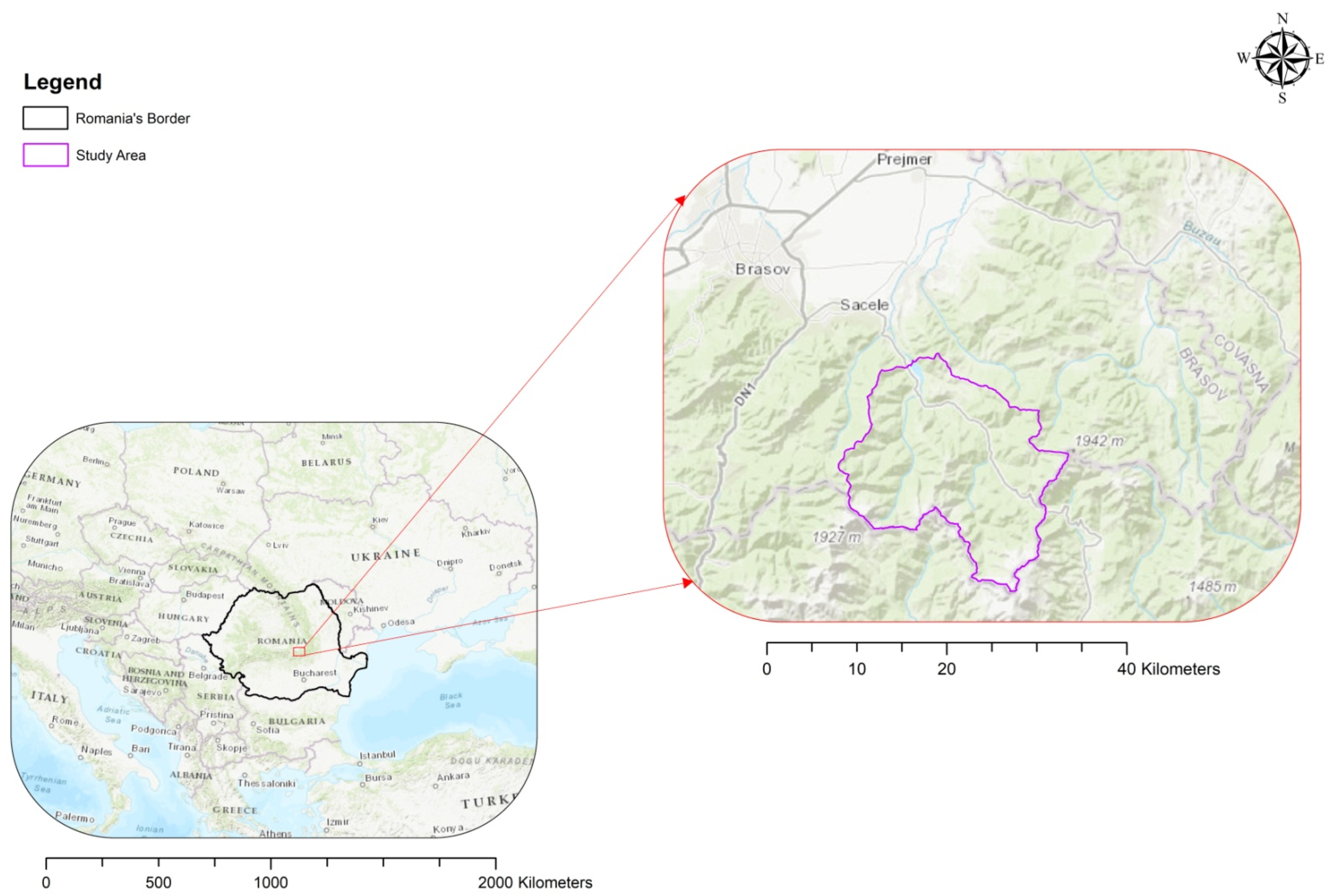
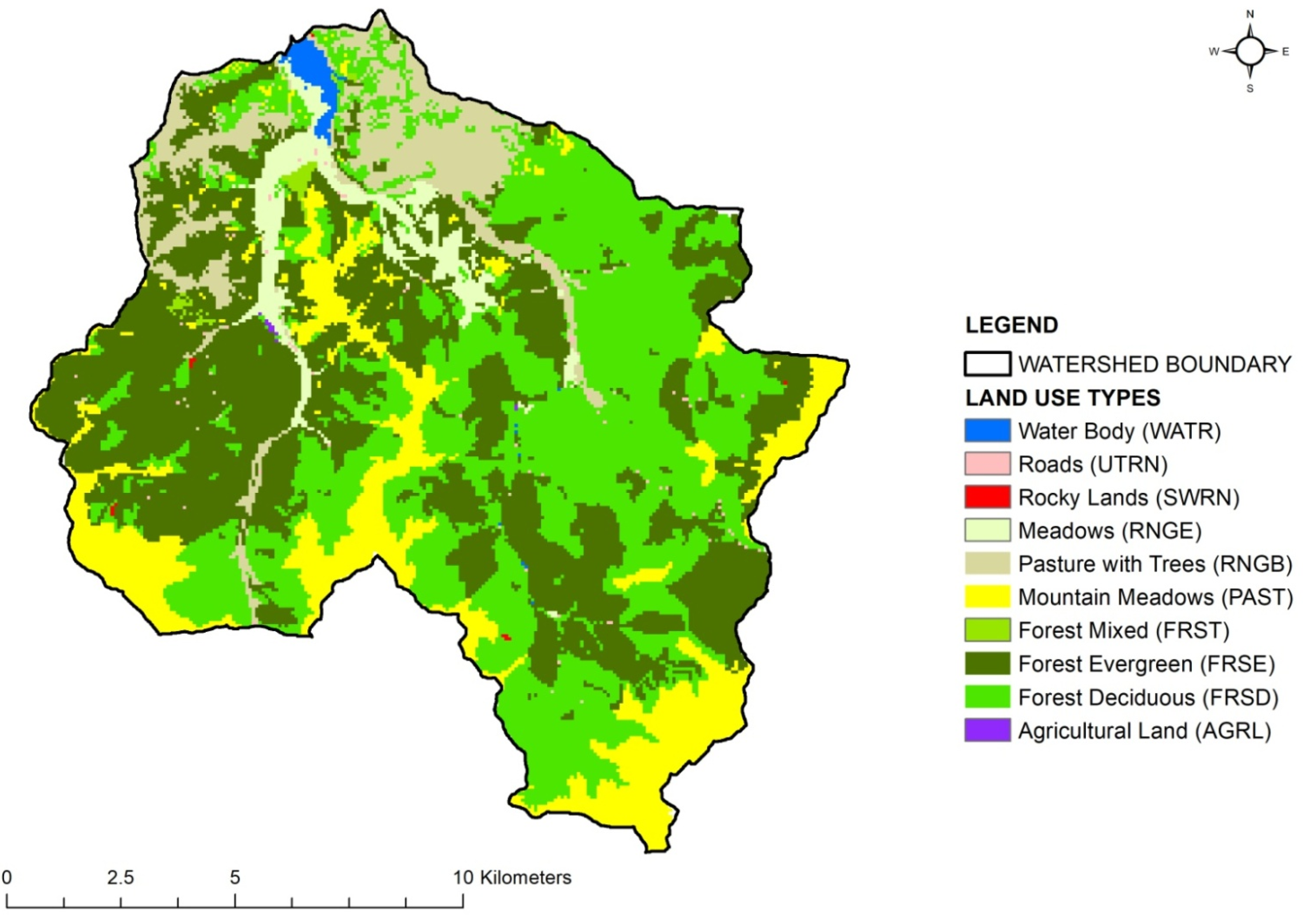
2.1. Study Area

The watershed is located in the central part of Romania (Figure 1) at 45°30′56″ N and 25°48′13″ E. Our research was performed in the Tărlung watershed upstream of the Săcele reservoir.

The watershed upstream of the Săcele reservoir covers 184 km² and represents the main source of water (90%) for the Brașov metropolitan area. The watershed elevation ranges between 724 and 1899 m. The study area is characterised by a continental climate that receives an annual precipitation of 700‒800 mm and records an average temperature of 4–5 °C. The main land use within the watershed is forests (73%), followed by mountain meadows (12% of the area), pastures with scattered trees (8%), pastures (2%), meadows (4%) and water bodies (1%). Regarding the soil types, 84% of the watershed soils are included in the cambisoil class, followed by spodisols (11%), cernisols (2%) and protisols (1%).

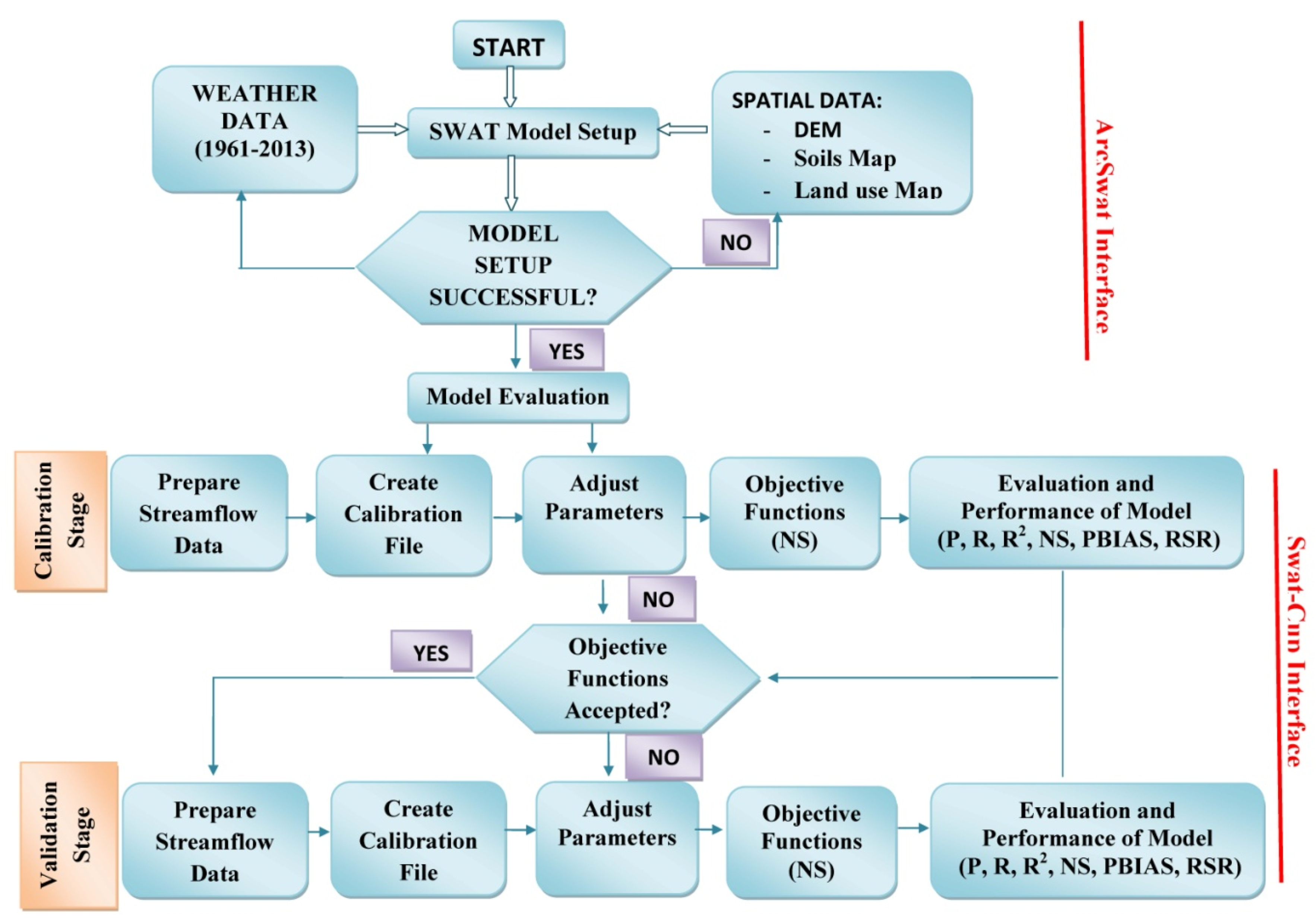
2.2. SWAT Hydrological Model

SWAT is a basin-scale model that operates at a daily time step and is extensively used in gauged and ungauged watersheds to simulate long-term hydrological processes under different drivers [45]. The model divides watersheds into sub-basins, which subsequently are delineated into multiple hydrological response units (HRUs) in agreement with homogeneous characteristics of soils, slopes and land use [46]. Thus, a more accurate physiographic description of the watershed will be ensured [1]. The model has a default database, but it also enables users to create a personalised database for the request inputs: soil, land use and weather database [47]. The flowchart to run the SWAT model is highlighted in Figure 2.

The model is an open-source software with low parameter requirements that enables users to customise their database and define elevation bands to adjust the orographic effect on precipitation and temperature, particularly for watersheds located in mountainous regions [46]. Moreover, for each elevation band, SWAT estimates accumulation, sublimation and snow melt [35] parameters with a large influence on hydrological processes within those river basins [36,49].

2.3. Model Parameterisation

To setup SWAT, four components are needed: The digital elevation model (DEM), weather, soil and a land use database. All model input data in vector and raster format (namely DEM, land use and soil) are in the EPSG 3844 projection (the projected coordinate system for Romania), datum Pulkovo 1942 (58)/Stereo70. DEM is the first and most important input considering that defining all the watershed characteristics relies on this component. We used a DEM with a 10-meter spatial resolution for our study, characterised by a 10-meter horizontal resolution and 5-meter vertical resolution. DEM has been supplied by the National Institute of Hydrology and Water Management (INHGA database). Using the ArcSWAT interface (an ArcGIS extension tool), the Tărlung watershed was delineated. Afterwards, we continued with HRU delineation by overlapping three spatial characteristics: land use, soil maps and slope. This procedure is based on similar characteristics of land use, soil and slopes that are lumped together after a threshold set by the user. For the Tărlung watershed, we established a threshold level of 10% each for soil, slope and land use to minimise errors due to multiple HRUs covering minimal surfaces. The action allows the reallocation at the sub-basin level of those three basic characteristics, which cover areas lower than the threshold value [50]. In doing so, the studied watershed was delineated into 169 sub-basins and 2419 HRUs. Moreover, to encapsulate the orographic influence and obtain accurate results, we defined ten elevation bands. After stream delineation, the morphological parameters and flow direction were obtained at the sub-watershed level.

Weather data are the second input requested by the SWAT model. For our research, we utilised data retrieved from the ROCADA dataset V 1.0 [51,52] and covered the 1961–2013 period. ROCADA represents a state-of-the-art homogenised gridded climatic dataset encompassing Romania at a spatial resolution of 0.1°. This database has been used and its accuracy has been confirmed in many studies [53,54]. We also two used other patchy datasets regarding precipitation (1988–2010) and river discharge (1974–2015) that were recorded inside of the watershed (Babarunca and Săcele Reservoir hydrometric stations). The river discharge measurements were used to calibrate and validate the model and minimise the model’s uncertainty. These two hydrometric stations belong to the INHGA that provided us with the river discharge datasets. The INHGA is empowered to provide hydrological data for different types of research and development projects. The weather database comprises the precipitation, minimum and maximum temperature, average wind speed, solar radiation and relative humidity and was conceived in a particular format accepted by SWAT, and afterwards embedded in the model and used for performing simulations.

The soil database was updated based on the information retrieved from the forest and pastoral management plans (Forest Management Plan 2009 and 2013, Silvopastoral Management Plan 1989) compiled for the Tărlung watershed by the National Institute for Research and Development in Forestry (INCDS) database. The maps enclosed in the aforementioned studies were used to identify the spatial distribution of the soil types within the studied watershed (Figure 3). The database was developed at the forest management compartment level in vector format and subsequently converted into raster format.

Due to time and money constraints, we did not have information regarding some soil characteristics like bulk density (SOL_BD), hydraulic conductivity (SOL_K) and water content (SOL_AWC) required when building the SWAT model. Instead, we used the soil-plant-atmosphere-water model (SPAW), an open-source software [55]. The SPAW program automatically determines those parameters according to certain soil properties like organic matter, sand and clay percentage. The value of each soil characteristic was inserted into the SPAW application, which automatically delivered water content, bulk density and hydraulic conductivity for each soil layer. Other parameters like soil albedo (SOL_ALB) and soil erodibility factor (K_USLE) were computed considering the research performed by [56,57], respectively. After determining all the required parameters regarding soil characteristics, the user soil table was completed (Table S1). To connect the default database and the raster of soil types at the watershed level, we created a table (user soil .txt format) with codes for each soil type. The codes can be found both at the raster level and in the SWAT default database. Finally, the user soil table was fed into the model and soils were reclassified in agreement with the SWAT codes. Subsequently, soil types were classified by hydrological groups. This classification was made considering the research performed by [58] in accordance with sand and clay percentage and soil layer depth. The soils within the watershed were framed in two hydrological groups, namely Group B (90.57%) and Group C (9.43%), which are characterised by medium and low infiltration capacity, respectively [59].

The land use database was updated using the information collected from the management plans alluded to above and observations on satellite images regarding roads, buildings and water bodies. The dominant land use categories (Figure 4) identified in the watershed were forests (73%), followed by mountain meadows (12%) and pastures with scattered trees (8%). Small percentages within the watershed area were occupied by meadows (4%), pastures (2%) and water bodies (1%).

The land use look-up table was designed in the requested format (.txt file) and was uploaded in the model, and afterwards, the land use was reclassified accordingly with the codes defined in ArcSWAT. Soil and land databases were developed at the forest management unit level. After building the requested databases and feeding them into the model, we set SWAT to run at a monthly time step for the 1961–2013 period (i.e., 53 years). This procedure also implied setting a warm-up period, namely 1961–1965, a length of time following the recommendations regarding the warm-up period setting for hydrologic models [60]. Hence, we obtained the hydrological parameters at the sub-basin level for 48 years and were also able to identify potential errors.

2.4. Model Performance Evaluation Criteria

The performance of the SWAT model was automatically carried out using the SWAT-CUP software [61]. We selected the SUFI-2 (Sequential Uncertainty Fitting version 2) algorithm from the four distinct procedures provided by SWAT-CUP due to its ability to optimise the parameters with minimal repetitions [44]. Another advantage is that this procedure considers both the model uncertainty and the uncertainty between the SWAT parameters and those that are measured [61]. The following widely applied parameters in hydrological studies were used for evaluating the model performance [62]: The coefficient of determination (R²), percent bias (PBIAS), standard deviation rate (RSR) and Nash Sutcliffe Model Efficiency (NSE). Choosing a multiple statistics indicator has to “increase the likelihood of mixed interpretation of model performance” [63]. R² reflects the degree of co-linearity amongst simulated and observed values and is computed using Equation (1) [64]. This index ranges between 0 and 1, where 0 describes no correlation, while 1 shows a good agreement:

$${\mathrm{R}}^2=\frac{[{{\displaystyle \sum }}_{\mathrm{i}=1}^{\mathrm{n}}\left({\mathrm{Q}}_{\mathrm{obs}}-{\mathrm{Q}}_{\mathrm{obs},\mathrm{m}}\right){\left({\mathrm{Q}}_{\mathrm{sim}}-{\mathrm{Q}}_{\mathrm{sim},\mathrm{m}}\right)]}^2}{{[{{\displaystyle \sum }}_{\mathrm{i}=1}^{\mathrm{n}}{\left({\mathrm{Q}}_{\mathrm{obs}}-{\mathrm{Q}}_{\mathrm{obs},\mathrm{m}}\right)}^2{{\displaystyle \sum }}_{\mathrm{i}=1}^{\mathrm{n}}\left({\mathrm{Q}}_{\mathrm{sim}}-{\mathrm{Q}}_{\mathrm{sim},\mathrm{m}}\right)]}^2}$$

(1)

where Q_obs is the discharge measured, Q_sim is the discharge simulated, Q_{obs, m} is the mean of measured discharge, and Q_{sim, m} is the mean of simulated discharge.

PBIAS calculates the model errors [65]. Expressed in percentage after using Equation (2), the good fit of the model is indicated through values close to 0 [66]. The underestimation of the model results is highlighted by positive simulated PBIAS values, while negative simulated values suggest overestimation [63]:

$$\mathrm{PBIAS}=\frac{{{\displaystyle \sum }}_{\mathrm{i}=1}^{\mathrm{n}}\left({\mathrm{Y}}_{\mathrm{i}}^{\mathrm{obs}}-{\mathrm{Y}}_{\mathrm{i}}^{\mathrm{sim}}\right)\ast \left(100\right)}{{{\displaystyle \sum }}_{\mathrm{i}=1}^{\mathrm{n}}\left({\mathrm{Y}}_{\mathrm{i}}^{\mathrm{obs}}\right)}$$

(2)

where Y^obs is the measured value of considered variable, Y^sim is the simulated value of considered variable.

RSR is computed as the ratio between root mean square error (RMSE) and standard deviation of observed values (STEDEV_obs) using Equation (3) [63]. A value close to 0 of this parameter indicates a perfect model simulation [63]:

$$\mathrm{RSR}=\frac{\mathrm{RMSE}}{{\mathrm{STEDEV}}_{\mathrm{obs}}}=\frac{\left[\sqrt{{{\displaystyle \sum }}_{\mathrm{i}=1}^{\mathrm{n}}{\left({\mathrm{Y}}_{\mathrm{i}}^{\mathrm{obs}}-{\mathrm{Y}}_{\mathrm{i}}^{\mathrm{sim}}\right)}^2}\right]}{\left[\sqrt{{{\displaystyle \sum }}_{\mathrm{i}=1}^{\mathrm{n}}{\left({\mathrm{Y}}_{\mathrm{i}}^{\mathrm{obs}}-{\mathrm{Y}}_{\mathrm{i}}^{\mathrm{mean}}\right)}^2}\right]}$$

(3)

where Y^obs is the measured value of considered variable, Y^sim is the simulated value of considered variable, Y^mean is the mean of the measured and simulated value.

NSE highlights the 1:1 fit between observed and simulated values using Equation (4) [67]:

$$\mathrm{NSE}=\frac{{\left[{{\displaystyle \sum }}_{\mathrm{i}=1}^{\mathrm{n}}\left({\mathrm{Q}}_{\mathrm{sim}}-{\mathrm{Q}}_{\mathrm{obs}}\right)\right]}^2}{{\left[{{\displaystyle \sum }}_{\mathrm{i}=1}^{\mathrm{n}}\left({\mathrm{Q}}_{\mathrm{obs}}-{\mathrm{Q}}_{\mathrm{obs},\mathrm{m}}\right)\right]}^2}$$

(4)

where Q_sim is the discharge simulated, Q_obs is the discharge measured and Q_{obs, m} is the mean of measured discharge.

Additionally, the model performance was evaluated using the p-factor and r-factor. The p-factor indicates the fraction of data bracketed by the 95PPu band, while the r-factor represents the ratio of the average width of the 95PPu band and the standard deviation of the measured variable [68,69,70]. For p-factor, better values are higher than 0.7, while for r-factor values between 0.7–1.5 are recommended [68,69,70].

3. Results

3.1. Sensitivity Analysis

The sensitivity analysis aims to identify the parameters with the largest influence on model outputs, thus influencing its successful application. Undertaken before calibration, this procedure has the role of identifying key parameters that subsequently will be used in model calibration [71]. The sensitivity analysis is a mathematical technique applied to enable users to examine how variations in the outputs of a numerical model can be attributed to variations of its inputs [45]. Alongside calibration and validation, this procedure is decisive for minimising the output uncertainty and efficiently perform the simulations [71]. The sensitivity analysis uses a t-test to assess the relative parameter significance, while the p-value indicates the sensitivity rank. After performing the global sensitivity analysis, the parameters with large t-test values and smallest p-values are the most sensitive [72]. We considered 12 parameters (defined in

Table 1. The default range and adjusted values of parameters included in the calibration procedure.

Parameter	Description	Variation Method	Minimum and Maximum Value	Adjusted Value
First calibration performed for parameters that insert water into the system
SFTMP.bsn	Snowfall temperature	Replace	−20…20	−4.791781
SMFMX.bsn	Maximum melt rate for snow during year	Replace	0…20	13.605089
SMFMN.bsn	Minimum melt rate for snow during the year	Replace	0…20	6.092970
SMTMP.bsn	Snow melt base temperature	Replace	−20…20	2.299827
CANMX.hru_FRSE	Maximum canopy storage for forest evergreen	Replace	0…100	2.149979
CANMX.hru_FRSD	Maximum canopy storage for forest deciduous	Replace	0…100	4.746581
CANMX.hru_PAST	Maximum canopy storage for pastures	Replace	0…100	4.563951
Second calibration performed for chosen parameters
CN2.mgt	SCS runoff curve number (-)	Multiply	−0.20…0.20	0.120750
ESCO.hru	Soil evaporation compensation factor	Replace	0…1	0.506750
EPCO.hru	Plant uptake compensation factor (-)	Replace	0…1	0.337250
HRU_SLP.hru	Average slope steepness (m/m)	Multiply	0…1	0.597250
OV_N.hru	Manning’s “n” value for overland flow (-)	Multiply	−0.20…0.00	−0.078850
GW_REVAP.gw	Coefficient for groundwater revap (days)	Replace	0.02…0.2	0.165935
GW_DELAY.gw	Groundwater delay time (days)	Replace	0…500	496.875000
ALPHA_BF.gw	Base flow alpha factor (1/days)	Replace	0…1	0.640750
RCHRG_DP.gw	Deep aquifer percolation fraction (-)	Multiply	0…1	0.899750
REVAPMN.gw	Threshold depth of water in the shallow aquifer for revap or percolation (mm)	Replace	0…500	132.875000
GWQMN.gw	Threshold depth of water in the shallow aquifer for return flow (mm)	Replace	0…5000	288.750000
SURLAG.bsn	Surface runoff lag time	Replace	0.05…24	10.847938
SOL_BD(1).sol	Moist bulk density	Multiply	0.9…2.5	0.047175
SOL_K(1).sol	Saturated hydraulic conductivity (mm/hr)	Multiply	−0.80…0.80	−0.410800
SOL_AWC(1).sol	Available water capacity of the soil layer (mmH2O/mm soil)	Multiply	−0.20…0.10	−0.175625
CH_N2.rte	Manning’s “n” value for the main channel	Replace	−0.01…0.3	0.119475
CH_K2.rte	Effective hydraulic conductivity in main channel alluvium	Replace	−0.01…500	172.625000

) with the largest influence on model outputs: CN2, REVAPMN, GW_DELAY, SOL_K, ESCO, GWQMN, CH_N2, CH_K2, GW_REVAP, ALPHA_BF, LAT_TIME and SOL_BD.

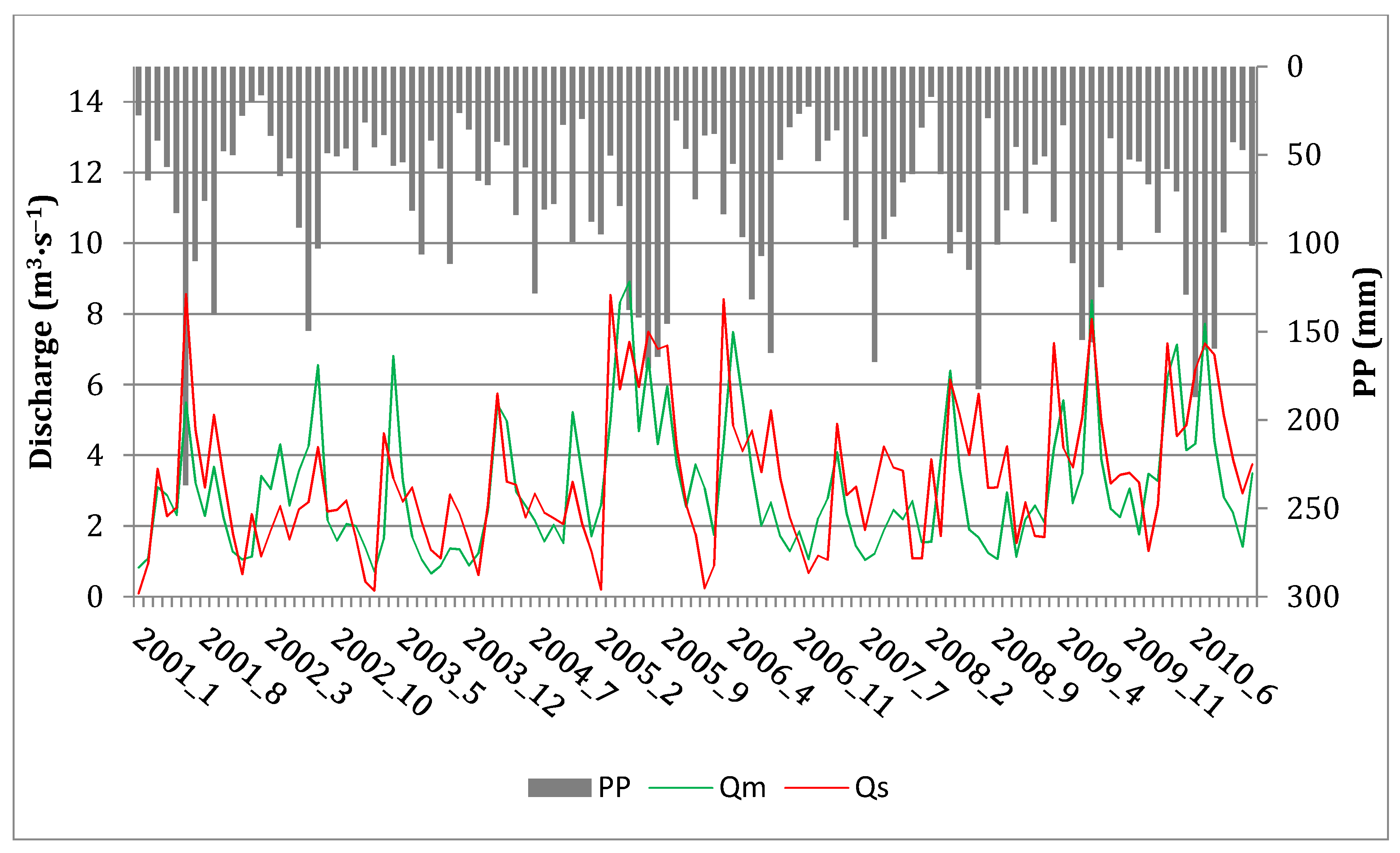
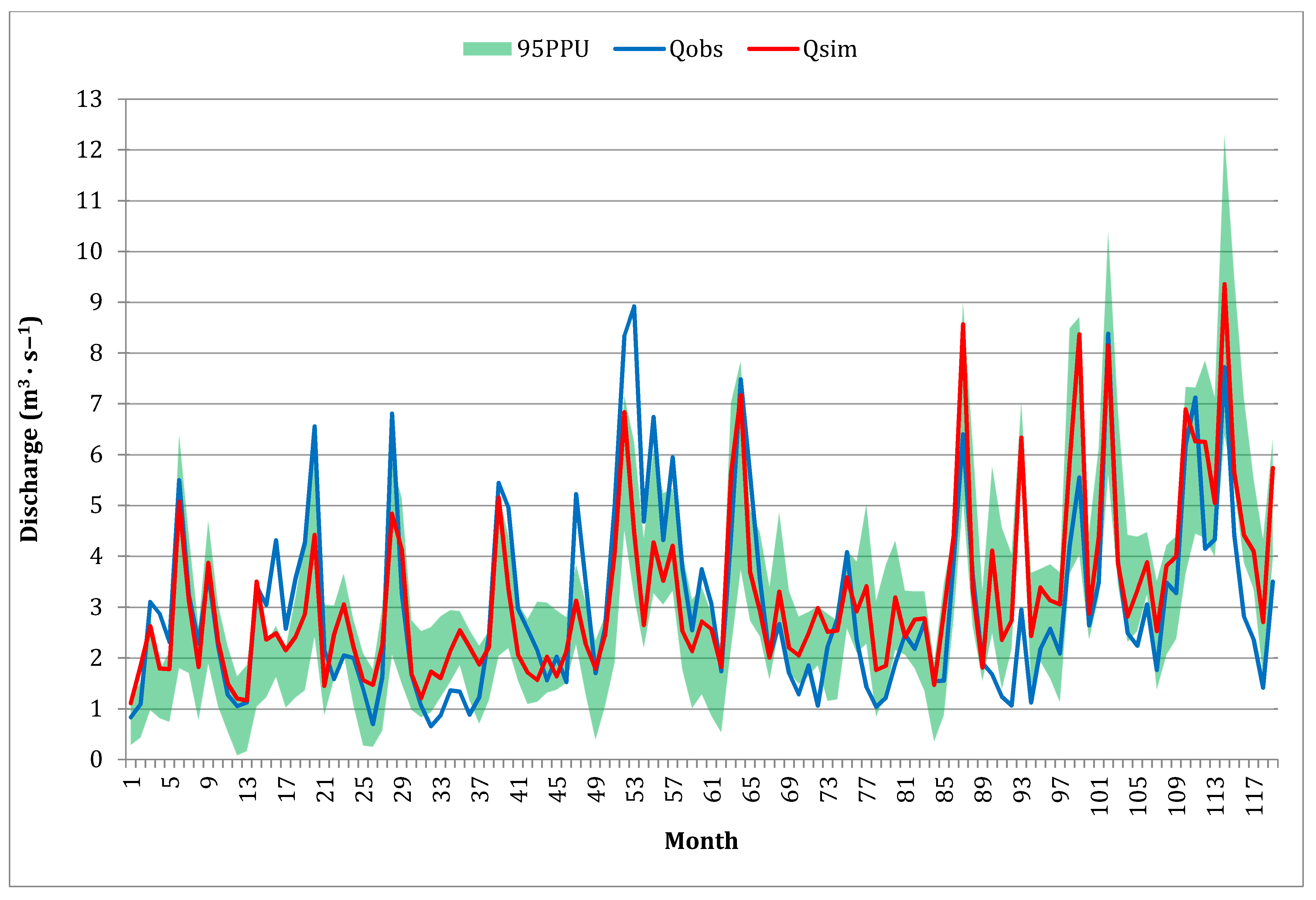
3.2. Model Calibration

After sensitivity analysis, we performed the calibration procedure to minimise the discrepancies amongst simulated data and recorded values [73]. The automatic calibration was also conducted using the SWAT-CUP program under the SUFI-2 algorithm. The model performance was assessed in agreement with the model performance evaluation criteria alluded to above.

The calibration was done for 2001–2010. This period was chosen due to continuous measurements and the dry, average and wet years necessary to ensure a high model performance with a lower uncertainty in the predictions [74]. Previously, we set up a five-year warm-up period (1996–2000) requested for model initialisation [61]. In doing so, we obtained the monthly river discharge for 10 years (Figure 5).

To obtain the best estimates between simulated and observed flow (Figure 6), we used the parallel processing module and performed seven iterations of 2000 simulations each. The process stopped when the model achieved a good performance rating indicated by the values of the statistical parameters recommended by [63], which can be accepted and used for assessing future impacts.

The parameters that insert water into the system (e.g., snowmelt or canopy storage parameters) should be calibrated independently from the other parameters [73]. Therefore, we performed the first calibration, including only SFTMP, SMTMP, SMFMX, SMFMN, TIMP and CANMX parameters, and ran the model until the statistical indices reached the performance rating recommended [63]. After those parameters were adjusted and fixed, they were subsequently excluded for the following calibration simulations. The second calibration was done independently for the first one and for 17 parameters that concerned only the parameters related to soil, groundwater, watershed and management characteristics. The selected parameters, the default range and their adjusted values are given in Table 1. Similar to the first calibration, the procedure was repeated until the statistical indices met the performance level that proves model acceptance.

Overall, the calibration procedure revealed a satisfactory SWAT performance, indicated by the statistical parameter values, appraised after [63], namely: R² = 0.61 (satisfactory), NSE = 0.59 (satisfactory), RSR = 0.64 (satisfactory), PBIAS = −5.7, p-factor = 0.72, and r-factor = 1.22. Hence, the SWAT performance was satisfactory to very good, and the obtained values revealed the model acceptance for simulating hydrological processes within the Tărlung watershed.

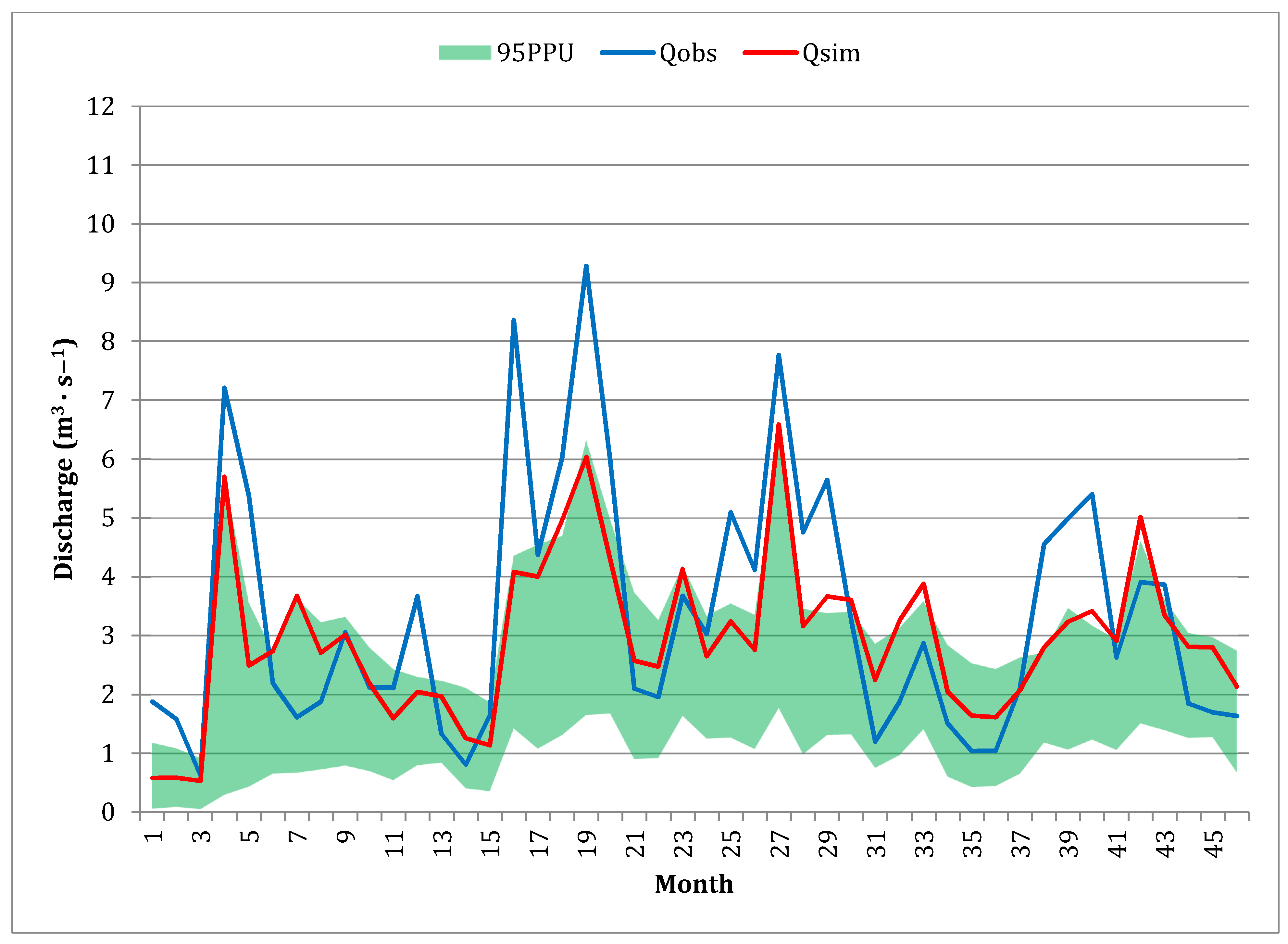
3.3. Model Validation

The validation confirms the results obtained after calibration [73]. This stage is important for ensuring the accuracy of the outputs considering that these will be further used in the decision process [75]. In our study, the validation was carried out for the same parameters used in calibration and considering the 1996–1999 period after previously setting up a five-year period for model warm-up. The period adopted for validation followed the same characteristics as in the calibration, namely continuous river discharges measurements and the presence of wet, dry and average years. For obtaining the best estimates between simulated and observed river discharge during validation, we performed a single iteration of 2000 simulations (Figure 7).

Nonetheless, if the user performs more than one iteration, it will increase the uncertainty of the model output due to the iterative character of the SUFI-2 algorithm [69]. The model efficiency was assessed using the same statistical indices as in the calibration. For those indices we obtained the following values appraised in accordance with the recommended performance rating [63]: R² = 0.78 (very good), NSE = 0.62 (satisfactory), RSR = 0.62 (satisfactory), p-factor = 0.67 and r-factor = 1.22. Overall, the model performance was satisfactory to very good, and the validation procedure results indicate that SWAT is suitable for assessing future impacts within the Tărlung watershed.

4. Discussion

The SWAT model developed particularly for large watersheds was applied, for the first time, both to the case study area and nationwide for a small-sized watershed. In this respect, we first customised the SWAT database to the local specificity of the studied region. In the next step, we performed the sensitivity analysis procedure that reduces the time required for calibration. During this stage, the parameters with the largest influences on hydrological processes are identified. In doing so, it was revealed that snowmelt and canopy retention are parameters with large influences on water balance within the Tărlung watershed. Those parameters have triggered lately, in the mountainous area, perilous floods during the spring months [48], particularly when snowmelt is overlapped with rainfall [38]. Due to their meaningful influence on hydrological process parameters that directly insert water into the system, they should not be calibrated together with other parameters (e.g., groundwater delay time, the coefficient for groundwater revap, base flow alpha factor and so on) because, as [73] states, they can generate identifiability issues. Therefore, snowmelt and canopy retention parameters were calibrated separately from the rest of the parameters that describe the watershed characteristics. In this respect, the first calibration includes only the snowmelt and canopy retention parameters, and the second calibration was made only for parameters that illustrate the watershed characteristics. Comparing the maximum canopy storage (CANMX) for evergreen forests and deciduous forests, the lower value was obtained for evergreen forests (see Table 1). A similar situation was also reported by [76]. However, the maximum canopy storage of deciduous forests is quite similar to the value obtained for pasture (see Table 1). This result agrees with the findings reported by [77], who obtained for pastures a maximum canopy storage even higher than those obtained for forests. In the case study area, an extension of pasture will affect the water quality due to the turbidity increments. These increments are also favoured by the main soil types from the watershed (Eutric Cambisol and Dystric Cambisol), which have high percentages of clay and silt (see Table S1), particles that are retained longer in suspension and affect the quality of water [1]. Thus, the water treatment capacity of the water plant will be exceeded and the water demand will not be covered (as has previously happened in the case study area). To prevent turbidity increments, the decision-makers should consider promoting “close to nature” forest management. This management practice will help preserve biodiversity and achieve the objectives highlighted and promoted in the EU’s Biodiversity Strategy for 2030 [78].

Afterwards, the model performance was appraised through calibration and validation procedures that provided a satisfactory rating. This result indicates that the hydrological processes within the Tărlung watershed are well captured. After performing both procedures we noticed that the values of R² and NSE parameters increased in the validation compared with calibration. This is an unusual situation because the optimisation of parameters occurs during the first procedure, but this circumstance has been reported in other research [22,66,79,80,81]. This situation may be due to the symmetry regression of the SWAT model [80], the number of wet or dry years included in both procedures or most likely due to the iterative character of the model [79,80,81]. The model uncertainties were assessed through p-factor and r-factor. The values obtained for the p-factor showed that the 95PPU band envelops 72% of the measured river discharges in the calibration and 67% during validation. Those results indicate a minimum uncertainty for calibration compared with validation. Although the p-factor value during validation was 0.67 (slightly less than the lower limit of the interval recommended in the literature), we preserved this result. We did not perform another iteration because this repetition would have increased the uncertainty of the model results [73]. The r-factor represents the thicknesses of the 95PPU envelope and was 1.22 both for calibration and validation. According to [61], the values obtained for these two indices during both procedures revealed lower uncertainties in model results. Overall, the SWAT performance evaluated using the R², NSE, RSR, and PBIAS showed a satisfactory model performance.

After running the SWAT model, both overestimations and underestimations at the monthly level were revealed (see Figure 6). The most meaningful overestimations were observed during the spring season (e.g., March 2003, 2005, 2006, 2009) and can be attributed to the fast snowmelt process [17,38,80,82,83,84,85]. Overestimations were also noticed during the summer season after heavy rainfall events, with similar results being reported by other authors [11,86,87]. The most significant underestimations were noticed during May in 2003, 2005, 2006 and 2010. These deficiencies can be generated by rainfall spatial variability within the watershed [86,88] and underline the necessity of research infrastructure installation that is properly spatially distributed to capture the spatial variability of rainfalls inside the watershed with high accuracy. Another consequence can be an inaccurate simulation of some parameters included in the water balance equation like groundwater and evapotranspiration [89], highlighting the importance of using field measurements.

Nevertheless, the SWAT model proved its performance and reliability and is suitable scientific support for decision-makers in planning activities, particularly in watersheds located in mountainous regions. These environments are important sources of freshwater, food, energy and biodiversity, and therefore enhancing their resilience is imperative under climate and land use change [24]. This task is a priority mentioned in the SDG 15: “Protect, restore and promote sustainable use of terrestrial ecosystems, sustainably manage forests, combat desertification, and halt and reverse land degradation and halt biodiversity loss”. SDG’s target is in 15.4 “By 2030, ensure the conservation of mountain ecosystems, including their biodiversity, in order to enhance their capacity to provide benefits that are essential for sustainable development” [90]. Considering that mountain areas host 23% of the total forests [24], their protection will alleviate climate change effects [78]. Furthermore, the “Framework convention on the protection and sustainable development of the Carpathians,” signed by our country, also highlights the importance of mountainous regions for all ecosystems and the role of the local community to achieve an integrated and balanced sustainability of these environments [91]. Therefore, the calibrated and validated SWAT model can be considered a valuable planning tool for designing action plans for small watersheds, which are currently neglected.

5. Conclusions

This research is an effort that can be considered a novel step for future studies investigating the hydrological behaviour of small watersheds. We presented the methodology used for customising the SWAT model to the local specificity for testing its ability to simulate the hydrological processes within a small forested ungauged watershed located in a mountainous region. The studied watershed has meaningful importance for Brașov city and its surrounding areas because it represents the main drinking and industrial water source. Future climate change projections published for the 21^st century underline the importance of conducting such hydrological assessments to investigate watershed behaviour under climate-related risks. Therefore, we focused on testing, for the first time (nationwide and for a small forested watershed), the applicability of the SWAT hydrological model in a small watershed located in a mountainous area. Given that we built a detailed and customised database, the calibration and validation procedures revealed that SWAT meets the requirements and is adequate to simulate the hydrological processes within the Tărlung watershed. The model was developed for large river basins and had certain deficiencies reported in the literature. Nevertheless, this study stresses the importance of several factors (e.g., the accuracy of input data, choosing the proper interval for performing the model’s calibration and validation procedures, and carefully selecting the parameters to perform those procedures) that contribute and ensure the SWAT’s suitability for application in small ungauged watersheds. After running the SWAT model for 53 years, we noticed a good agreement in mirroring the hydrological process, which is accurately captured within the watershed. The contribution of this paper enables the local upgraded SWAT model to be further used as a guidance tool for management decisions that pursue sustainable and integrated watershed management under multiple challenges (climate, environmental and societal).

References

1. Jabbar, F.K.; Grote, K. Evaluation of the predictive reliability of a new watershed health assessment method using the SWAT model. Environ. Monit. Assess. 2020, 192. [Google Scholar] [CrossRef] [PubMed]
2. Deshmukh, A.; Singh, R. Physio-climatic controls on vulnerability of watersheds to climate and land use change across the US. Water Resour. Res. 2016, 52, 8775–8793. [Google Scholar] [CrossRef]
3. IPCC. Summary for Policymakers: Climate Change 2014: Impacts, Adaptation and Vulnerability. Part A: Global and Sectoral Aspects. Contributions of the Working Group II to the Fifth Assessment Report. 2014. [Google Scholar]
4. Guerreiro, S.B.; Dawson, R.J.; Kilsby, C.; Lewis, E.; Ford, A. Future heat-waves, droughts and floods in 571 European cities. Environ. Res. Lett. 2018, 13. [Google Scholar] [CrossRef]
5. Miller, J.D.; Immerzeel, W.W.; Rees, G. Climate change impacts on glacier hydrology and river discharge in the Hindu Kush-Himalayas. Mt. Res. Dev. 2012, 32, 461–467. [Google Scholar] [CrossRef] [Green Version]
6. Song, Y.; Park, Y.; Lee, J.; Park, M.; Song, Y. Flood forecasting and warning system structures: Procedure and application to a small urban stream in South Korea. Water 2019, 11, 1571. [Google Scholar] [CrossRef] [Green Version]
7. Duan, Y.; Meng, F.; Liu, T.; Huang, Y.; Luo, M.; Xing, W.; De Maeyer, P. Sub-daily simulation of mountain flood processes based on the modified soil water assessment tool (Swat) model. Int. J. Environ. Res. Public Health 2019, 16, 3118. [Google Scholar] [CrossRef] [PubMed] [Green Version]
8. Weiskopf, S.R.; Rubenstein, M.A.; Crozier, L.G.; Gaichas, S.; Griffis, R.; Halofsky, J.E.; Hyde, K.J.W.; Morelli, T.L.; Morisette, J.T.; Muñoz, R.C.; et al. Climate change effects on biodiversity, ecosystems, ecosystem services, and natural resource management in the United States. Sci. Total Environ. 2020, 733, 137782. [Google Scholar] [CrossRef]
9. Cui, T.; Yang, T.; Xu, C.Y.; Shao, Q.; Wang, X.; Li, Z. Assessment of the impact of climate change on flow regime at multiple temporal scales and potential ecological implications in an alpine river. Stoch. Environ. Res. Risk Assess. 2018, 32, 1849–1866. [Google Scholar] [CrossRef]
10. Senent-Aparicio, J.; Liu, S.; Pérez-Sánchez, J.; López-Ballesteros, A.; Jimeno-Sáez, P. Assessing Impacts of Climate Variability and Reforestation Activities on Water Resources in the Headwaters of the Segura River Basin (SE Spain). Sustainability 2018, 10, 3277. [Google Scholar] [CrossRef] [Green Version]
11. Grey, O.P.; St G Webber, D.F.; Setegn, S.G.; Melesse, A.M. Application of the Soil and Water Assessment Tool (SWAT Model) on a small tropical island (Great River Watershed, Jamaica) as a tool in Integrated Watershed and Coastal Zone Management. Rev. Biol. Trop. Int. J. Trop. Biol. Conserv. 2014, 62, 293–305. [Google Scholar]
12. Orozco, I.; Martínez, A.; Ortega, V. Assessment of the water, environmental, economic and social vulnerability of a watershed to the potential effects of climate change and land use change. Water 2020, 12, 1682. [Google Scholar] [CrossRef]
13. Marin, M.; Clinciu, I.; Tudose, N.; Ungurean, C.; Adorjani, A.; Mihalache, A.; Davidescu, A.; Davidescu, Ș.O.; Dinca, L.; Cacovean, H. Assessing the vulnerability of water resources in the context of climate changes in a small forested watershed using SWAT: A review. Environ. Res. 2020, 184, 109330. [Google Scholar] [CrossRef]
14. Berezowski, T.; Chybicki, A. High-resolution discharge forecasting for snowmelt and rainfall mixed events. Water 2018, 10, 56. [Google Scholar] [CrossRef] [Green Version]
15. Jurik, Ĺ.; Húska, D.; Halászová, K.; Bandlerová, A. Small water reservoirs—Sources of water or problems? J. Ecol. Eng. 2015, 16, 22–28. [Google Scholar] [CrossRef]
16. Cai, X.; Wallington, K.; Shafiee-Jood, M.; Marston, L. Understanding and managing the food-energy-water nexus—Opportunities for water resources research. Adv. Water Resour. 2018, 111, 259–273. [Google Scholar] [CrossRef]
17. Mengistu, A.G.; van Rensburg, L.D.; Woyessa, Y.E. Techniques for calibration and validation of SWAT model in data scarce arid and semi-arid catchments in South Africa. J. Hydrol. Reg. Stud. 2019, 25, 100621. [Google Scholar] [CrossRef]
18. Osei, M.A.; Amekudzi, L.K.; Wemegah, D.D.; Preko, K.; Gyawu, E.S.; Obiri-Danso, K. The impact of climate and land-use changes on the hydrological processes of Owabi catchment from SWAT analysis. J. Hydrol. Reg. Stud. 2019, 25, 100620. [Google Scholar] [CrossRef]
19. Chen, Q.; Chen, H.; Wang, J.; Zhao, Y.; Chen, J.; Xu, C. Impacts of Climate Change and Land-Use Change on Hydrological Extremes in the Jinsha River Basin. Water 2019, 11, 1398. [Google Scholar] [CrossRef] [Green Version]
20. Yan, R.; Cai, Y.; Li, C.; Wang, X.; Liu, Q. Hydrological Responses to Climate and Land Use Changes in a Watershed of the Loess Plateau, China. Sustainability 2019, 11, 1443. [Google Scholar] [CrossRef] [Green Version]
21. Phung, Q.A.; Thompson, A.L.; Baffaut, C.; Costello, C.; Sadler, E.J.; Svoma, B.M.; Lupo, A.; Gautam, S. Climate and Land Use Effects on Hydrologic Processes in a Primarily Rain-Fed, Agricultural Watershed. JAWRA J. Am. Water Resour. Assoc. 2019, 55, 1196–1215. [Google Scholar] [CrossRef]
22. Esmali, A.; Golshan, M.; Kavian, A. Investigating the performance of SWAT and IHACRES in simulation streamflow under different climatic regions in Iran. Atmósfera 2021, 34, 79–96. [Google Scholar] [CrossRef] [Green Version]
23. Beniston, M. Climatic change in mountain regions: A review of possible impacts. Clim. Change 2003, 59, 5–31. [Google Scholar] [CrossRef]
24. Mountain Partnership. Mountains and the Sustainable Development Goals. 2014. Available online: http://www.fao.org/fileadmin/templates/mountain_partnership/doc/POLICY_BRIEFS/Mountains_and_the_Sustainable_Development_Goals_-_NY_-_8Jan.2014.pdf (accessed on 15 March 2021).
25. BIO Intelligence Service. Literature Review on the Potential Climate Change Effects on Drinking Water Resources across the EU and the Identification of Priorities among Different Types of Drinking Water Supplies, Final Report—ADWICE Project Prepared for European Commission DG Environment, 20–22 Villa Deshayes, 75014 Paris. 2012. Available online: https://ec.europa.eu/environment/archives/water/adaptation/pdf/ADWICE_FinalReport.pdf (accessed on 15 March 2021).
26. Jacob, D.; Petersen, J.; Eggert, B.; Alias, A.; Christensen, O.B.; Bouwer, L.M.; Braun, A.; Colette, A.; Déqué, M.; Georgievski, G.; et al. EURO-CORDEX: New high-resolution climate change projections for European impact research. Reg. Environ. Chang. 2014, 14, 563–578. [Google Scholar] [CrossRef]
27. Kotlarski, S.; Keuler, K.; Christensen, O.B.; Colette, A.; Déqué, M.; Gobiet, A.; Goergen, K.; Jacob, D.; Lüthi, D.; Van Meijgaard, E.; et al. Regional climate modeling on European scales: A joint standard evaluation of the EURO-CORDEX RCM ensemble. Geosci. Model Dev. 2014, 7, 1297–1333. [Google Scholar] [CrossRef] [Green Version]
28. Downing, J.A. Emerging global role of small lakes and ponds: Little things mean a lot. Limnetica 2010, 29, 9–24. [Google Scholar] [CrossRef]
29. Hackenbruch, J.; Kunz-Plapp, T.; Müller, S.; Schipper, J.W. Tailoring climate parameters to information needs for local adaptation to climate change. Climate 2017, 5, 25. [Google Scholar] [CrossRef] [Green Version]
30. Bayabil, H.K.; Dile, Y.T. Improving hydrologic simulations of a small watershed through soil data integration. Water 2020, 12, 2763. [Google Scholar] [CrossRef]
31. Irving, K.; Kuemmerlen, M.; Kiesel, J.; Kakouei, K.; Domisch, S.; Jähnig, S.C. Data descriptor: A high-resolution streamflow and hydrological metrics dataset for ecological modeling using a regression model. Sci. Data 2018, 5, 1–14. [Google Scholar] [CrossRef]
32. Zhao, Q.; Zhu, Y.; Wan, D.; Yu, Y.; Lu, Y. Similarity Analysis of Small- and Medium-Sized Watersheds Based on Clustering Ensemble Model. Water 2019, 12, 69. [Google Scholar] [CrossRef] [Green Version]
33. Rahman, K.; Maringanti, C.; Beniston, M.; Widmer, F.; Abbaspour, K.; Lehmann, A. Streamflow Modeling in a Highly Managed Mountainous Glacier Watershed Using SWAT: The Upper Rhone River Watershed Case in Switzerland. Water Resour. Manag. 2013, 27, 323–339. [Google Scholar] [CrossRef] [Green Version]
34. Arora, M.; Kumar, R.; Kumar, N.; Malhotra, J. Hydrological modeling and streamflow characterization of Gangotri Glacier. In Geostatistical and Geospatial Approaches for the Characterization of Natural Resources in the Environment: Challenges, Processes and Strategies, IAMG 2014; Capital Publishing Company: New Delhi, India, 2016. [Google Scholar]
35. Jain, S.; Jain, S.; Jain, N.; Xu, C.-Y. Hydrologic modeling of a Himalayan mountain basin by using the SWAT mode. Hydrol. Earth Syst. Sci. Discuss. 2017. [Google Scholar] [CrossRef] [Green Version]
36. Mateo-Lázaro, J.; Castillo-Mateo, J.; Sánchez-Navarro, J.Á.; Fuertes-Rodríguez, V.; García-Gil, A.; Edo-Romero, V. Assessment of the role of snowmelt in a flood event in a gauged catchment. Water 2019, 11, 506. [Google Scholar] [CrossRef] [Green Version]
37. Romanescu, G.; Jora, I.; Stoleriu, C. The most important high floods in Vaslui river basin -causes and consequences. Carpathian J. Earth Environ. Sci. 2011, 6, 119–132. [Google Scholar]
38. Birsan, M.V.; Zaharia, L.; Chendes, V.; Branescu, E. Recent trends in streamflow in Romania (1976-2005). Rom. Reports Phys. 2012, 64, 275–280. [Google Scholar]
39. The World Bank. Romania, Climate Change and Low Carbon Green Growth Program, Component B Sector Report, Forest Sector Rapid Assessment. 2014. Available online: https://openknowledge.worldbank.org/bitstream/handle/10986/17570/842620WP0P14660Box0382136B00PUBLIC0.pdf?sequence=1&isAllowed=y (accessed on 1 March 2021).
40. Yang, L.; Smith, J.A.; Baeck, M.L.; Zhang, Y. Flash flooding in small urban watersheds: Storm event hydrologic response. Water Resour. Res. 2016, 52, 4571–4589. [Google Scholar] [CrossRef] [Green Version]
41. Kvočka, D.; Ahmadian, R.; Falconer, R.A. Predicting Flood Hazard Indices in Torrential or Flashy River Basins and Catchments. Water Resour. Manag. 2018, 32, 2335–2352. [Google Scholar] [CrossRef] [Green Version]
42. Petroselli, A.; Grimaldi, S. Design hydrograph estimation in small and fully ungauged basins: A preliminary assessment of the EBA4SUB framework. J. Flood Risk Manag. 2018, 11, S197–S210. [Google Scholar] [CrossRef]
43. Apollonio, C.; Bruno, M.F.; Iemmolo, G.; Molfetta, M.G.; Pellicani, R. Flood Risk Evaluation in Ungauged Coastal Areas. Water 2020, 5, 1466. [Google Scholar] [CrossRef]
44. Ha, L.; Bastiaanssen, W.; van Griensven, A.; van Dijk, A.; Senay, G. SWAT-CUP for Calibration of Spatially Distributed Hydrological Processes and Ecosystem Services in a Vietnamese River Basin Using Remote Sensing. Hydrol. Earth Syst. Sci. Discuss. 2017. [Google Scholar] [CrossRef] [Green Version]
45. Arnold, J.G.; Moriasi, D.N.; Gassman, P.W.; Abbaspour, K.C.; White, M.J.; Srinivasan, R.; Santhi, C.; Harmel, R.D.; Van Griensven, A.; Van Liew, M.W.; et al. SWAT: Model use, calibration, and validation. Trans. ASABE 2012, 55, 1491–1508. [Google Scholar] [CrossRef]
46. Neitsch, S.; Arnold, J.; Kiniry, J.; Williams, J. Neitsch Grassland, Soil, Water Research Laboratory; Agricultural Research Service Blackland Research Center; Texas AgriLife Research. Soil & Water Assessment Tool, Theoretical Documentation Version 2009. Texas Water Resources Institute. exas Water Resources Institute Technical Report No. 365 Texas A&M University System College Station, Texas 77843-2118. 2011. [Google Scholar] [CrossRef]
47. Neitsch, S.L.; Arnold, J.G.; Kiniry, J.R.; Williams, J.R. Soil and Water Assessment Tool Theoretical Documentation Version 2005; Grassland, Soil and Water Research Laboratory, Agricultural Research Service: Temple, TX, USA, 2005. [Google Scholar]
48. Tudose, N.C.; Davidescu, S.O.; Cheval, S.; Chendes, V.; Ungurean, C.; Babata, M. Integrated Model of River Basin, Land Use and Urban Water Supply. Deliverable 3.4. CLISWELN Project. 2018. Available online: https://ms.hereon.de/imperia/md/content/csc/projekte/projekte/clisweln_d3.4_romania_study_case_final-2.pdf (accessed on 9 November 2020).
49. Noor, H.; Vafakhah, M.; Taheriyoun, M.; Moghadasi, M. Hydrology modelling in Taleghan mountainous watershed using SWAT. J. Water L. Dev. 2014, 20, 11–18. [Google Scholar] [CrossRef]
50. Winchell, M.; Srinivasan, R.; Di Luzio, M.; Arnold, J. ArcSWAT 2.3.4 Interface for SWAT2005: User’s Guide, Version September 2009. Texas Agricultural Experiment Station and Agricultural Research Service- US Department of Agriculture, Temple. 2009. [Google Scholar]
51. Bîrsan, M.-V.; Dumitrescu, A. ROCADA: Romanian daily gridded climatic dataset (1961-2013) V1.0. Nat. Hazards 2014, 78, 1045–1063. [Google Scholar] [CrossRef]
52. Dumitrescu, A.; Birsan, M.V. ROCADA: A gridded daily climatic dataset over Romania (1961–2013) for nine meteorological variables. Nat. Hazards 2015, 78, 1045–1063. [Google Scholar] [CrossRef]
53. Popa, I.; Badea, O.; Silaghi, D. Influence of climate on tree health evaluated by defoliation in the ICP level I network (Romania). IForest 2017, 10, 554–560. [Google Scholar] [CrossRef]
54. Sfîcă, L.; Croitoru, A.E.; Iordache, I.; Ciupertea, A.F. Synoptic conditions generating heatwaves and warm spells in Romania. Atmosphere 2017, 8, 50. [Google Scholar] [CrossRef] [Green Version]
55. Karim, T.H.; Fattah, M.A. Efficiency of the SPAW model in estimation of saturated hydraulic conductivity in calcareous soils. J. Univ. Duhok 2020, 23, 189–201. [Google Scholar] [CrossRef]
56. Post, D.F.; Fimbres, A.; Matthias, A.D.; Sano, E.E.; Accioly, L.; Batchily, A.K.; Ferreira, L.G. Predicting Soil Albedo from Soil Color and Spectral Reflectance Data. Soil Sci. Soc. Am. J. 2000, 64, 1027–1034. [Google Scholar] [CrossRef]
57. Williams, J.R. The EPIC Model. In Computer Models of Watershed Hydrology; Singh, V.P., Ed.; Water Resources Publications: Highlands Ranch, CO, USA, 1995; ISBN 0918334918. [Google Scholar]
58. Gijsman, A.J.; Thornton, P.K.; Hoogenboom, G. Using the WISE database to parameterize soil inputs for crop simulation models. Comput. Electron. Agric. 2007, 56, 85–100. [Google Scholar] [CrossRef]
59. Arnold, J.G.; Kiniry, J.R.; Srinivasan, R.; Williams, J.R.; Haney, E.B.; Neitsch, S.L. Input/Output Documentation. 2012. Available online: https://swat.tamu.edu/media/69296/swat-io-documentation-2012.pdf (accessed on 20 November 2020).
60. Daggupati, P.; Pai, N.; Ale, S.; Douglas-Mankin, K.R.; Zeckoski, R.W.; Jeong, J.; Parajuli, P.B.; Saraswat, D.; Youssef, M.A. A recommended calibration and validation strategy for hydrologic and water quality models. Trans. ASABE 2015, 58, 1705–1719. [Google Scholar] [CrossRef] [Green Version]
61. Abbaspour, K.C. SWAT-CUP. SWAT Calibration and Uncertainty Programs. 2015, p. 100. Available online: https://swat.tamu.edu/media/114860/usermanual_swatcup.pdf (accessed on 6 December 2020).
62. Harmel, R.D.; Smith, P.K.; Migliaccio, K.W.; Chaubey, I.; Douglas-Mankin, K.R.; Benham, B.; Shukla, S.; Muñoz-Carpena, R.; Robson, B.J. Evaluating, interpreting, and communicating performance of hydrologic/water quality models considering intended use: A review and recommendatrions. Environ. Model. Softw. 2014, 21, 40–51. [Google Scholar]
63. Moriasi, D.N.; Arnold, J.G.; Van Liew, M.W.; Bingner, R.L.; Harmel, R.D.; Veith, T.L. Model evaluation guidelines for systematic quantification of accuracy in watershed simulations. Trans. ASABE 2007, 50, 885–900. [Google Scholar] [CrossRef]
64. Moriasi, D.N.; Gitau, M.W.; Pai, N.; Daggupati, P. Hydrologic and water quality models: Performance measures and evaluation criteria. Trans. ASABE 2015, 58, 1763–1785. [Google Scholar] [CrossRef] [Green Version]
65. Gupta, H.V.; Sorooshian, S.; Yapo, P.O. Status of Automatic Calibration for Hydrologic Models: Comparison with Multilevel Expert Calibration. J. Hydrol. Eng. 1999, 4, 135–143. [Google Scholar] [CrossRef]
66. da Silva, M.G.; de Aguiar Netto, A.O.; de Jesus Neves, R.J.; do Vasco, A.N.; Almeida, C.; Faccioli, G.G. Sensitivity Analysis and Calibration of Hydrological Modeling of the Watershed Northeast Brazil. J. Environ. Prot. 2015, 6, 837–850. [Google Scholar] [CrossRef] [Green Version]
67. Nash, J.E.; Sutcliffe, J.V. River flow forecasting through conceptual models part I - A discussion of principles. J. Hydrol. 1970, 10, 282–290. [Google Scholar] [CrossRef]
68. Abbaspour, K.C.; Johnson, C.A.; Th van Genuchten, M. Estimating Uncertain Flow and Transport Parameters Using a Sequential Uncertainty Fitting Procedure. Vadose Zone J. 2004, 3, 1340–1352. [Google Scholar] [CrossRef]
69. Abbaspour, K.C.; Rouholahnejad, E.; Vaghefi, S.; Srinivasan, R.; Yang, H.; Kløve, B. A continental-scale hydrology and water quality model for Europe: Calibration and uncertainty of a high-resolution large-scale SWAT model. J. Hydrol. 2015, 524, 733–752. [Google Scholar] [CrossRef] [Green Version]
70. Thavhana, M.P.; Savage, M.J.; Moeletsi, M.E. SWAT model uncertainty analysis, calibration and validation for runoff simulation in the Luvuvhu River catchment, South Africa. Phys. Chem. Earth 2018, 105, 115–124. [Google Scholar] [CrossRef]
71. Qiu, L.J.; Zheng, F.L.; Yin, R.S. SWAT-based runoff and sediment simulation in a small watershed, the loessial hilly-gullied region of China: Capabilities and challenges. Int. J. Sediment Res. 2012, 27, 226–234. [Google Scholar] [CrossRef]
72. Emam, R.A.; Kappas, M.; Hoang Khanh Nguyen, L.; Renchin, T. Hydrological Modeling in an Ungauged Basin of Central Vietnam Using SWAT Model. Hydrol. Earth Syst. Sci. Discuss. 2016, 1–33. [Google Scholar] [CrossRef] [Green Version]
73. Abbaspour, K.C.; Vaghefi, S.A.; Srinivasan, R. A guideline for successful calibration and uncertainty analysis for soil and water assessment: A review of papers from the 2016 international SWAT conference. Water 2017, 10, 6. [Google Scholar] [CrossRef] [Green Version]
74. Abbaspour, K.C.; Yang, J.; Maximov, I.; Siber, R.; Bogner, K.; Mieleitner, J.; Zobrist, J.; Srinivasan, R. Modelling hydrology and water quality in the pre-alpine/alpine Thur watershed using SWAT. J. Hydrol. 2007, 333, 413–430. [Google Scholar] [CrossRef]
75. Wallace, C.W.; Flanagan, D.C.; Engel, B.A. Evaluating the effects ofwatershed size on SWAT calibration. Water 2018, 10, 898. [Google Scholar] [CrossRef] [Green Version]
76. Miralles, D.G.; Gash, J.H.; Holmes, T.R.H.; De Jeu, R.A.M.; Dolman, A.J. Global canopy interception from satellite observations. J. Geophys. Res. Atmos. 2010, 115, 1–8. [Google Scholar] [CrossRef]
77. Cui, Y.; Jia, L.; Hu, G.; Zhou, J. Mapping of interception loss of vegetation in the heihe river basin of china using remote sensing observations. IEEE Geosci. Remote Sens. Lett. 2015, 12, 23–27. [Google Scholar] [CrossRef]
78. European Commission. Communication from the Commission to the European Parliament, the Council, the European Economic and Social Committee and the Committee of the Regions. 2020. Available online: https://eur-lex.europa.eu/resource.html?uri=cellar:a3c806a6-9ab3-11ea-9d2d-01aa75ed71a1.0001.02/DOC_1&format=PDF (accessed on 13 January 2021).
79. Brouziyne, Y.; Abouabdillah, A.; Bouabid, R.; Benaabidate, L. SWAT streamflow modeling for hydrological components’ understanding within an agro-sylvo-pastoral watershed in Morocco. J. Mater. Environ. Sci. 2018, 9, 128–138. [Google Scholar] [CrossRef]
80. Aawar, T.; Khare, D. Assessment of climate change impacts on streamflow through hydrological model using SWAT model: A case study of Afghanistan. Model. Earth Syst. Environ. 2020, 6, 1427–1437. [Google Scholar] [CrossRef]
81. Leng, M.; Yu, Y.; Wang, S.; Zhang, Z. Simulating the hydrological processes of a meso-scalewatershed on the Loess Plateau, China. Water 2020, 12, 878. [Google Scholar] [CrossRef] [Green Version]
82. Amatya, D.M.; Jha, M.K. Evaluating the SWAT model for a low-gradient forested watershed in coastal South Carolina. Trans. ASABE 2011, 54, 2151–2163. [Google Scholar] [CrossRef] [Green Version]
83. Mapes, K.L.; Pricope, N.G. Evaluating SWAT model performance for runoff, percolation, and sediment loss estimation in low-gradientwatersheds of the Atlantic Coastal Plain. Hydrology 2020, 7, 21. [Google Scholar] [CrossRef] [Green Version]
84. Tolera, M.B.; Chung, I.M.; Chang, S.W. Evaluation of the climate forecast system reanalysis weather data for watershed modeling in Upper Awash Basin, ethiopia. Water 2018, 10, 725. [Google Scholar] [CrossRef] [Green Version]
85. Busico, G.; Colombani, N.; Fronzi, D.; Pellegrini, M.; Tazioli, A.; Mastrocicco, M. Evaluating SWAT model performance, considering different soils data input, to quantify actual and future runoff susceptibility in a highly urbanized basin. J. Environ. Manag. 2020, 266. [Google Scholar] [CrossRef]
86. Abbas, T.; Nabi, G.; Boota, M.W.; Hussain, F.; Azam, M.I.; Jin, H.; Faisal, M. Uncertainty analysis of runoff and sedimentation in a forested watershed using sequential uncertainty fitting method. Sci. Cold Arid Reg. 2016, 8, 297–310. [Google Scholar] [CrossRef]
87. Briones, R.U.; Ella, V.B.; Bantayan, N.C. Hydrologic impact evaluation of land use and land cover change in Palico Watershed, Batangas, Philippines Using the SWAT model. J. Environ. Sci. Manag. 2016, 19, 96–107. [Google Scholar]
88. Narsimlu, B.; Gosain, A.K.; Chahar, B.R.; Singh, S.K.; Srivastava, P.K. SWAT Model Calibration and Uncertainty Analysis for Streamflow Prediction in the Kunwari River Basin, India, Using Sequential Uncertainty Fitting. Environ. Process. 2015, 2, 79–95. [Google Scholar] [CrossRef]
89. Adhikary, P.P.; Sena, D.R.; Dash, C.J.; Mandal, U.; Nanda, S.; Madhu, M.; Sahoo, D.C.; Mishra, P.K. Effect of Calibration and Validation Decisions on Streamflow Modeling for a Heterogeneous and Low Runoff–Producing River Basin in India. J. Hydrol. Eng. 2019, 24, 05019015. [Google Scholar] [CrossRef]
90. United Nations Transforming Our World: The 2030 Agenda for Sustainable Development: Sustainable Development Knowledge Platform. Available online: https://sustainabledevelopment.un.org/post2015/transformingourworld (accessed on 12 June 2020).
91. Carpathian Framework Convention. Framework Convention on the Protection and Sustainable Development of the Carpathians. Available online: http://www.carpathianconvention.org/tl_files/carpathiancon/Downloads/01TheConvention/1.1.1.1_CarpathianConvention.pdf (accessed on 19 February 2021).
Figure 1. Study area location.
Forests 12 00860 g001
Figure 2. Diagram of SWAT model [48].
Forests 12 00860 g002
Figure 3. Soil types within the Tărlung watershed.
Forests 12 00860 g003
Figure 4. Land use at the Tărlung watershed level.
Forests 12 00860 g004
Figure 5. Simulated river discharge (Qs), measured river discharge (Qm) and precipitations (PP) for the Tărlung watershed for the 2001‒2010 period.
Forests 12 00860 g005
Figure 6. The 95PPU plot between observed and best simulated discharges after the calibration procedure.
Forests 12 00860 g006
Figure 7. The 95PPU plot between observed and best simulated discharges after the validation procedure.
Forests 12 00860 g007