Article

Useful Life of Prescribed Fires in a Southern Mediterranean Basin: An Application to Pinus pinaster Stands in the Sierra Morena Range

by
Juan Ramón Molina
*,
Macarena Ortega
and
Francisco Rodríguez y Silva
Forest Fire Laboratory, Department of Forest Engineering, Edificio Leonardo da Vinci, Campus de Rabanales, University of Córdoba, 14071 Cordoba, Spain
*
Author to whom correspondence should be addressed.
Forests 2021, 12(4), 486; https://doi.org/10.3390/f12040486
Submission received: 1 February 2021 / Revised: 11 April 2021 / Accepted: 12 April 2021 / Published: 15 April 2021

Abstract

:
Prescribed fire is a globally relevant fuel treatment for surface fuel management and wildfire hazard reduction. However, Mediterranean ecosystems are adapted to low and moderate fires; hence, the useful life of prescribed fires is limited. Useful life is defined as the effective rotation length of prescribed fires to mitigate fire spread based on critical surface intensity for crown combustion. In this sense, the useful life of a prescribed fire focuses on surface fuel dynamics and its potential fire behavior. In Pinus pinaster stands, the useful life can be established between 0 and 4 years. Canopy base height, time elapsed from the burning, postfire precipitation, and fine fuel moisture content during the burning were identified as the most important variables in postburn fuel dynamics. Other stand characteristics and postfire precipitation can improve the fine fuel and live fuel dynamics models. Our findings support prescribed fires as an effective fuel treatment in the medium term for forest fire prevention, according to stand characteristics and burning implementation conditions. In this sense, forest managers can use the proposed decision tree to identify the useful life of each prescribed fire based on fine fuel moisture content during burning implementation.

1. Introduction

Land-use changes, the abandonment of traditional forest uses, and climate change are increasing the frequency of large forest fires [1] as well as their economic impacts and suppression costs [2]. According to the policy of excluding fire [3], fire agencies devote their efforts to forest fire prevention activities using traditional fuel treatments such as brushing, clearing, thinning, pruning, chipping, mastication, controlled burnings, and prescribed fires. Fuel treatments are aimed at surface fuel reduction and the increase of vertical distance between surface fuel and canopy base height [4]. However, all these treatments may not be effective under extreme weather conditions, large fire fronts, eruptive behavior, and atmospheric downburst phenomena [1].
The use of prescribed fires as a preventive management tool is indeed an uncertain and controversial situation [5,6]. Some authors [7,8,9,10] have pointed to prescribed fires as a promising tool to mitigate wildfire impacts in forests and settlements. In this sense, an upward trend in prescribed fires has begun due to its low cost and additional firefighter training [9]. Although prescribed fires can be an effective treatment for fuel load reduction in Southern Europe, the actual application of this technique can be rather reduced in size, and, consequently, its effectiveness in relation to large fire suppression and confinement is limited [11,12].
The effectiveness of prescribed fires can only be guaranteed in the short term due to fast postfire recovery [8,13,14]. Nevertheless, differences can be found based on vegetation growth and fuel load accumulation according to the burning season [3]. While a rotation length of two years has been required by some ecosystems [15], the rotation length of Pinus pinaster Ait. in Southern Europe has been established between two and four years [16]. P. pinaster, which is widely distributed in the Mediterranean Basin [17], is adapted to low- and moderate-intensity fires [18]. Some studies have increased the rotation length of pine stands not only based on surface fuel reduction but also tree growth. In this sense, a rotation length between four and six years to achieve suitable surface fuel reduction and to avoid the loss of P. ponderosa growth has been suggested [19]. Other authors [8,20] have suggested a rotation length of seven years in conifers, according to the prescribed fire effectiveness.
Surface fuel reduction or undergrowth reduction using prescribed fires decreases the risk of crown fire combustion [3,4,8,21]. However, the major or minor prescribed fire effectiveness depends on the fuel model, fuel availability, the fire ignition pattern, and the composition and structure of the ecosystems. In other words, the prescribed fire effectiveness or the useful life of the prescribed fire depends on burn windows [4,6,20,22]. In Southern Europe, Cistus ladanifer L. is frequently the dominant understory species, mainly in low canopy closure forests with a high canopy gap presence. It is a pioneer species with an extensive soil seed bank that increases the germination percentage with fire heat transference [23]. The use of prescribed fires can promote fuel dynamics changes, tree regeneration patterns, and even the modification of understory composition [24]. If tree crowns are too much affected by thermal pruning or even tree mortality, these changes can be pronounced. Nevertheless, some researchers [25] have pointed out the lack of differences between brushing clearing and prescribed fire in Cistus spp. ecosystems from the fourth year.
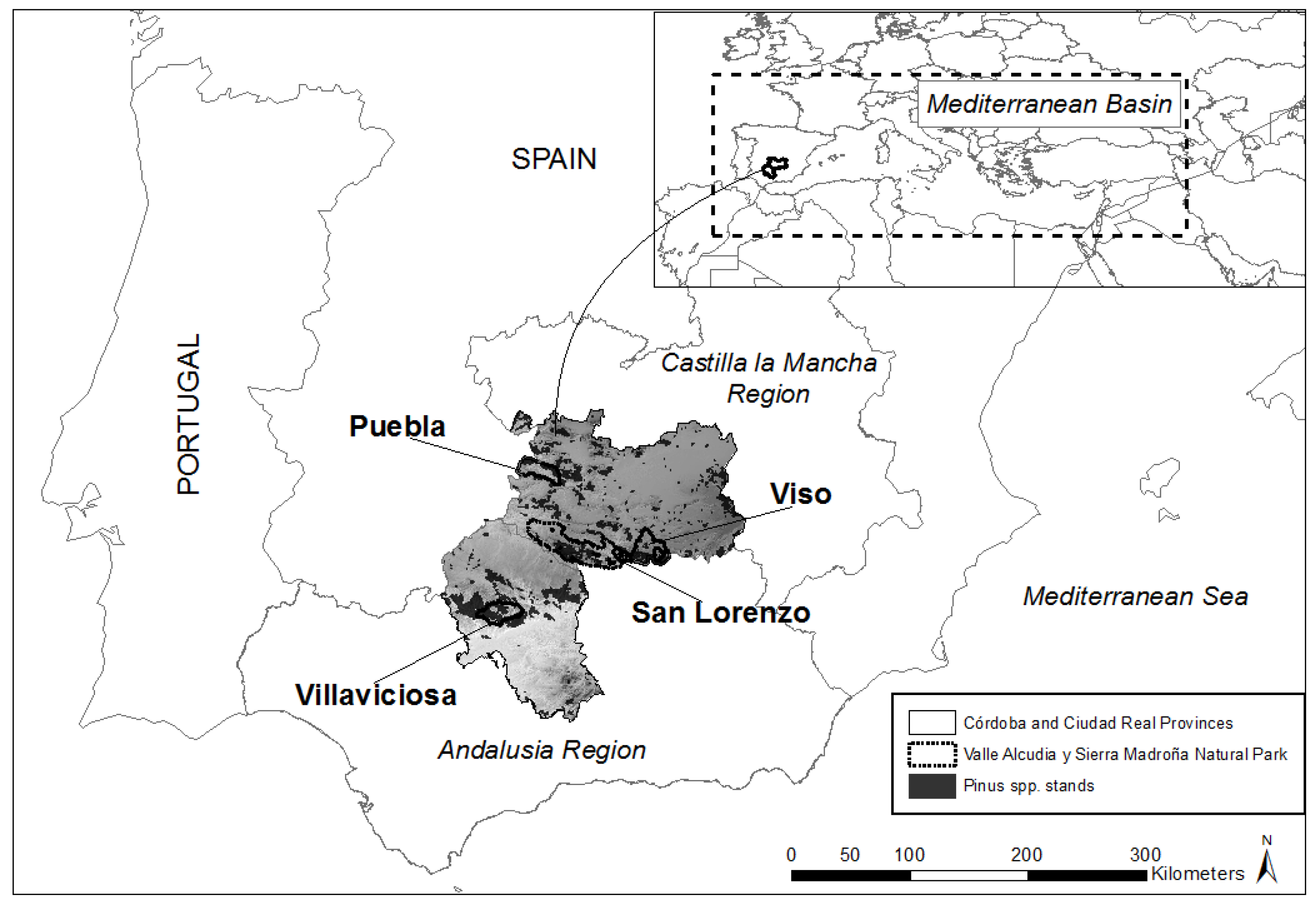
The aim of this research is the identification of the useful life of 11 maritime pine prescribed fires in Southern Europe. The useful life of a prescribed fire is defined as the effective rotation length based on fire behavior to prevent crown fire transition. In this sense, fire-line intensities below the critical surface intensity for crown combustion are needed. The analysis of prescribed fire effectiveness requires stand characterization, burning implementation conditions, and postfire surface and aerial fuel dynamics. Fuel characterization is based on a prefire inventory and periodical postfire inventories, including dynamic variables such as fuel load and canopy base height. Periodical fire behavior and the threshold for transition from surface fire to crown fire will be simulated according to the field inventory variables to identify the useful life of each prescribed fire. The knowledge of fuel dynamics, based on initial stand characteristics and burn window conditions, allows us to improve time–space fuel treatment efficiency and to manage the potential fuel dynamics of each stand according to their initial characteristics.

2. Materials and Methods

2.1. Study Area

This study was carried out in two provinces (Ciudad Real and Córdoba) in southern Spain (Figure 1). The four burning areas (San Lorenzo, Puebla, Viso, and Villaviciosa) are in one of the main mountain ranges in Spain, known as “Sierra Morena”. All the burning areas have a continental Mediterranean climate, with summer temperatures above 35 °C and summer relative humidity below 30%. These meteorological conditions predispose the vegetation to easy ignition and fire spread. The official statistics show an annual average of 109 forest fires in Ciudad Real and an annual average of 114 forest fires in Cordoba (period 1990–2019).
The study area comprises mature forests of P. pinaster with an understory dominated by C. ladanifer, accompanied by other flammable species such as C. albidus L., Rosmarinus officinalis L., and Genista hirsuta subsp. hirsuta Vahl. The fuel model is identified as fuel model 7/9/11 [26], model TU/TL/SB [27], or model HPM/HR/R [28], and, consequently, it is characterized by long-needle pine litter and slash, according to previous biomass harvesting. There is also a live-fuel presence due to the presence of canopy gaps that were promoted by biomass harvesting.
The 11 prescribed fires covered approximately 30 ha (Appendix A). The burnings were developed during the spring seasons between 2010 and 2016, according to different meteorological conditions and fire behaviors. The meteorological conditions were measured at 2-m above ground and inside the stand using two meteorological stations’ Skywatch Geos. The mean wind speed ranged from virtually zero to 12 km/h. In each burning, two destructive needle samplings of 100 g were taken and dried in an oven for 72 h at a temperature of 60 °C to calculate its real fuel moisture. In this sense, the fine fuel moisture content (FFMC) ranged from 9% to 14.5% in the Ciudad Real burnings and between 5% and 9% in the Cordoba burnings (Table 1). The fire ignition pattern was mainly strip-heading fire, except in the following burnings: San Lorenzo B, Puebla B, and Villaviciosa A (Table 1).
During the burning, not only meteorological and fuel availability conditions were collected, but also data on fire behavior. Telescopic range poles and a thermal camera (Flir Systems) were used to identify the flame length (FL) of each burning. FL was between 0.4–0.8 (San Lorenzo A and Puebla B) and 1.5–2.2 m (Viso D) (Table 1). We also used thermocouple type k of 1 mm to identify the rate of spread (ROS) and flame residence time (FRT) of each burning. In the prescribed fires carried out before 2014, we did not use the thermal camera and thermocouples because they were bought after that year. While ROS ranged from 0.2 (Villaviciosa A) and 6.75 m/min (Puebla C), FRT was between 72 (Viso C) and 310 s (Villaviciosa A) (as previously reported, FRT data is missing for the San Lorenzo A and San Lorenzo B burnings).

2.2. Field Inventory

The inventory was carried out using rounded plots of 1000 m2. The maximum error allowed from stand density was fixed at 30%, according to regional government recommendations [29]. In this sense, the inventory amounted to 59 sampling plots located across the different burnings (Appendix A). The sampling plots of the prescribed fires included both surface and canopy strata. UTM coordinates, species composition, and stand characteristics such as stand density, diameter at breast height, stand height, and canopy base height were identified (some variables can be seen in Table 2). While a Vertex clinometer allowed us to measure tree height and canopy base height, diameter at breast height was collected using a caliper. Canopy closure was calculated by multiplying the average crown projection area by stand density. Mean stand density was between 88 (Villaviciosa A) and 1210 trees/ha (Puebla A), and the diameter at breast height ranged from 18.1 (Puebla A) to 44.7 cm (Villaviciosa B). While the stand height was between 9 (San Lorenzo A) and 14.5 m (San Lorenzo B), the canopy base height ranged from 2 (Viso D) to 5.9 m (Puebla A, Puebla B, and Puebla C). The canopy closure varied from 40% (Villaviciosa A) to 90% (Puebla A).
In each sampling plot, three or four destructive samplings units of 1 m2 were collected using the line-intercept method [30]. The inventory amounted to 201 sampling units located across the different sampling plots (Appendix A). Surface fuel load was determined in these destructive sampling units, showing fuel load by category (live and dead) and particle size (1-, 10- and 100-h time lag). Although the soils of the study areas are very poor in humus content, L (litter layer), F (fermented litter layer), and H (humus layer) layers were included in the fine fuel load. In the case of the fine fuel load, moisture content differences were found between L, F, and H layers. Each fuel category sampling was oven-dried at 60 °C for 72 h to calculate its moisture content and to express fuel load as dry fuel load. The total prefire fuel load ranged from 10.68 (Villaviciosa A and Villaviciosa B) to 38 Mg/ha (San Lorenzo B) (Table 2). Fuel bed or litter depth is expressed as a mean value of four measures inside each sampling unit.

2.3. Postburn Fuel Dynamics

The postburn fuel load was determined periodically in sampling plots of 1 m2, showing fuel load by category (live and dead) and particle size (expressed in 1-, 10-, 100-h time lag). A minimum period of 12 months was established in the first postfire inventory to evaluate needles and branches fallen due to the thermal pruning effect. The studied burnings were developed between 2010 and 2016, so the time elapsed from the burning ranged from 42 (Puebla A, B, and C, and Viso C and D) to 84 months (San Lorenzo A). An agglomerative cluster analysis based on the Ward method was used to identify comparable pre- and postburn fuel loads. SPSS© software was used for this task and all statistical analyses.
Firstly, an asymptotic exponential model using T was used to predict fuel load accumulation. Principal component analysis (PCA) was applied to reduce the number of independent variables. Multiple linear and multiexponential analyses using a set of variables were also used to model the fuel load dynamics in P. pinaster stands. Strongly correlated variables (r > 0.7) were removed. If any variables without normal distribution were identified, a logarithmic transformation would have been used. The variables were used and classified into three groups:
  • Forest variables: stand density (SD), diameter at breast height (DBH), stand height (H), canopy base height (CBH), and canopy closure (CC).
  • Burning condition variables: wind speed measured at 2-m height during the burning (U2), FFMC during the burning, foliar moisture content (FMC), spread rate (ROS), flame length (FL), fire-line intensity (I), flame residence time (FRT), heat per unit area (H), fuel consumption (FC), scorch height (SHE), and scorch ratio (SR).
  • Meteorological variables: number of days with moderate or heavy wind in the six months postburn (wind speed >20 km/h) and number of days with heavy precipitation in the six months postburn (rain intensity >2 mm/h). Identification of the wind threshold was established using the Beaufort scale (the trees start to wave). In the case of precipitation, the State Meteorological Agency scale was used for no or weak rain.
Model reliability was determined by the coefficient of determination (>0.75), the standard error of estimation (SEE) and variables, and model significance (p < 0.05). Subsequently, an artificial neural network was applied to rank the relative and normalized influence of the significant variables attained from the regression analysis. Finally, we also used mixed linear modeling to account for the cofounded effect of various measurements per burn plot in TFL.

2.4. Useful Life of Prescribed Fires

We established two criteria to determine prescribed fire effectiveness. Firstly, in the stands with potential crown fire occurrence, prescribed fire effectiveness is identified as the rotation length to avoid the potential transition from surface fire to crown fire. In other words, the prescribed fire will be effective if the fire only spreads by surface fuel and, therefore, the fire will have lower intensity and suppression difficulty [31]. Secondly, in the stands without potential crown fire occurrence, prescribed fire effectiveness is understood as the rotation length to get an FL value lower than 1.5 m. This threshold was established according to suitable fire behavior for a direct firefighting attack with hand tools [32].
Fire behavior was identified based on ROS, HUA, I, FL and the threshold intensity for crown fire transition. These variables can be easily calculated using fire behavior simulators [33,34,35] that use semiempirical fire spread models (Table 3). ROS was calculated using the Rothermel model [36] for each burning and the time elapsed from the burning. The calculation of HUA and I was based on the formulations of [36,37], respectively (Table 3). FL was calculated using the model in [37]. Finally, threshold intensity for crown fire transition [38] depends on CBH and FMC. If the I value is higher than critical surface fire intensity, the threshold transition for crown fire will be reached.
Any fire behavior simulation in the medium- and long-term requires the creation of working scenarios according to meteorological conditions and postburn fuel dynamics. Meteorological scenarios were obtained from the closest weather station to each study area. The national dataset [39] was used for the last five summers (from 1 July 2015 to 31 August 2019). The 95% percentile of the maximum daily temperature, minimum daily relative humidity, and maximum daily wind speed was used to get the most extreme weather conditions that could generate crown fires. The 95% percentile proved to be useful in explaining the large forest fires in Southern Europe [40]. For the study period, the most unfavorable scenarios or combinations of 95% percentiles of temperature, relative humidity, and wind speed were registered on three different days (5 July 2015, 8 July 2015, and 5 August 2018). FFMC was based on the estimated temperature and relative humidity values, according to the model shown in Table 3. FMC was estimated based on a statistical analysis of the FMC dataset using permanent sampling plots of P. pinaster in Sierra Morena (unpublished data, 2011–2019).
Postburn simulations require the use of custom fuel modeling to predict fire behavior. We adjusted fuel model characteristics (total fuel load, fuel load by categories, fuel bed depth, and CBH) for each prescribed fire and period using our periodical field inventories. In some prescribed fires, such as in Villaviciosa A and Villaviciosa B, the live fuel increase resulted in a change of fuel model (Model 9 to Model 7, based on the Rothermel classification, or Model TL to Model TU, based on the Scott and Burgan classification). The surface-area-to-volume ratio ranged from 98 (100-h time-lag dead fuel) to 6562 1/m (1-h time-lag dead fuel) based on laboratory identification. The drag coefficient on wind speed for each stand was identified from our meteorological weather stations as ranging from 0.28 (Puebla A–Puebla C) to 0.72 (Villaviciosa A).

3. Results

3.1. Postburn Fuel Dynamics

Preburn inventories identified three typologies or fuel models based on the greater or lesser presence of slash from biomass harvesting:
  • Fuel model with a light presence of “duff layer or F layer” (2–5 cm) and slash and down woody fuel beneath a forest canopy with an isolated distribution. It can resemble Fuel Model 9 [26] or Fuel Model HR5 [28], with a fuel load ranging from 10.68 to 16.59 Mg/ha. In these stands, mechanical harvesting using a full tree system and tree forwarding operations were used.
  • Fuel model with a heavy presence of “duff layer” (5–8 cm) and slash and down woody fuel beneath a forest canopy with a mosaic distribution. It can resemble Fuel Model 9 [26] or Fuel Model HR7 [28], with a fuel load ranging from 24.18 to 25.67 Mg/ha. In these stands, mechanical harvesting using a cut-to-length logging system and tree skidding operations promoted the presence of masticated fuel.
  • Fuel model with a continuous presence of litter and slash, which provide fire spread continuity. It can be associated with Fuel Model 11 [26] or Fuel Model R2 [28], with a fuel load ranging from 32.3 to 38 Mg/ha. A great amount of slash has not been entirely removed or masticated.
The fuel loads dropped to a greater or lesser extent in the short term with the prescribed fire implementation. FC, immediately postburn, was between 46.64% (San Lorenzo A) and 96.65% (Villaviciosa A) (Table 4). In the medium term (four years), all sampling plots continued with fuel loads lower than preburn values, except in Villaviciosa A. In the former burning, a substantial increase of live fuel occurred from the third year onward (Figure 2). Although live fuel appeared in the medium term in seven burnings without its previous existence, live fuel load in Villaviciosa A reached 12.44 Mg/ha in the fifth year (Table 4). In San Lorenzo A, a high fuel load was observed from the first year because FC was only 46.44% (Table 4). In this sense, its initial fuel load was practically recovered in 42 months. Despite the fact that the fuel reductions in San Lorenzo B and Viso D from the first year were over 60% of the preburn load, they did not reach the rest of the sampling burnings (Figure 2). As an example, Viso B and Viso A obtained a reduction of initial fuel load over 54 months, from 81.22% to 72.08, respectively (Table 4).
The cluster analysis identified five burning groups, considering the evolution of total fuel load (TFL), fine fuel load (FFL), coarse fuel load (CFL), and live fuel load (LFL):
  • Group I (Puebla A, Puebla B, Viso A, Viso B, and Villaviciosa B): These are burnings where a notable TFL reduction (86.02 ± 5.29%) was reached in the first year. Subsequently, TFL slowly increased (1.64 ± 0.48 Mg/ha*year). All burnings had a preburn CBH higher than 4.5 m.
  • Group II (Puebla C and Viso C): These are burnings where a lower TFL reduction (71.05 ± 2.58%) was reached in the first year. Subsequently, TFL moderately increased (2.21 ± 0.19 Mg/ha*year) from the first year. The preburn CBH ranged from 3 (Viso C) to 5.9 m (Puebla C).
  • Group III (Villaviciosa A): This is a burning where a reduction in TFL was noticed (80.34%) a year after the burning. However, TFL strongly increased (4.53 Mg/ha*year) from the first year onward. The prefire CBH was 4.2 m.
  • Group IV (San Lorenzo A): This is a burning where a low TFL reduction (38.14%) was reached in the first year. In this case, TFL slowly increased (1.86 Mg/ha*year) from the first year onward. The prefire CBH was very low (2.3 m).
  • Group V (San Lorenzo B and Viso D): These are burnings where a moderate TFL reduction was reached based on the high amount of coarse woody fuel and fire behavior. TFL moderately increased (2.46 ± 2.15 Mg/ha*year) from the first year onward. The prefire CBH was equal to or lower than 2.3 m.
The greatest differences were observed between San Lorenzo A, San Lorenzo B, and Viso D and the rest of the studied prescribed fires (Figure 3). Similarly, a notable difference was found between the last two burnings (Group V) and the first (Group IV). It should also be stressed that the difference was greater between Group I and Groups II and III than between Group II and Group III (Figure 3).
The results of the asymptotic exponential model, using only T, are not very reliable according to the coefficient of determination and the standard error of the estimation (Table 5). According to principal component analysis (PCA), it was possible to explain 86.03% of the variance of the TFL load dynamics with as few as 4 components or variables. Six dynamic postburn models were obtained, with a determination coefficient higher than 0.75 (Table 5). The first two models refer to TFL dynamics, with a determination coefficient higher than 0.8.
Canopy base height (CBH), time elapsed from the burning (T), number of days with heavy precipitation in the six months postfire (P), and fine fuel moisture content (FFMC) were the most important independent variables in TFL (Figure 4). The incorporation of stand density (SD) improved the FFL dynamics model, according to its relative and normalized importance (Figure 4). Wind speed during the burning (U2) and fine fuel moisture content (FFMC) were also included in the CFL dynamics model based on their relative and normalized importance (Figure 4). The FFL dynamics from the first year depended on CBH and P due to the low relative and normalized importance of T (Table 5). Finally, CC was the most outstanding variable for LFL (Table 5).
The best mixed model for TFL was formed by three independent variables (CBH, T, and P) in a similar way to previous findings. In this sense, this statistical analysis had a standard error of estimation of 1.62. Therefore, it had a lower standard error of estimation than the previous multiexponential models (Table 6). The covariance of the residuals in the mixed model was 1.62 (±0.38).

3.2. Useful Life of Prescribed Fires

Statistical analysis to identify the 95% percentile of the different study areas showed temperatures between 39.30 (Puebla A) and 40.62 °C (San Lorenzo A, San Lorenzo B, Viso A, Viso B, Viso C, and Viso D) and relative humidity ranging from 6.44% (San Lorenzo A, San Lorenzo B, Viso A, Viso B, Viso C, and Viso D) to 7.80% (Puebla A, Puebla B, and Puebla C). FFMC varied between 4.60% (San Lorenzo A, San Lorenzo B, Viso A, Viso B, Viso C, and Viso D) and 4.90% (Puebla A, Puebla B, and Puebla C) using the 95% percentile. Fermented litter moisture (F layer) ranged from 14.74% to 15.44%. The maximum wind speed was between 29.17 (Puebla A, Puebla B, and Puebla C) and 35.64 km/h (Villaviciosa A and Villaviciosa B) (wind speed was measured at 10-m above ground and outside the stand). Finally, FMC for maritime pine was estimated at 98.87% (unpublished data, 2011–2019), which coincided with similar weather conditions identified in the 95% percentile.
As stated previously, all fuel loads decreased with the prescribed fire implementation. Modifications in the different fuel typology dynamics were also included in the respective potential fire behavior simulations. The fuel bed depth (L, F, and H layers) ranged from 1 (Villaviciosa A and Villaviciosa B) to 25 cm (Viso D). The understory height from 42 months was between 0.05–0.1 cm (Puebla B and Viso C) and 1.1 m (Viso D). While the scorch height ranged from 2.5 (San Lorenzo B) to 9 m (Puebla A), the crown scorch ratio was between 3.9% (San Lorenzo B) and 43.86% (Puebla A) (Table 4). In this sense, the canopy base height increased between 0.2 (San Lorenzo B) and 3.1 m (Puebla A and Villaviciosa A) (comparative analysis of Table 2 and Table 4).
Fire behavior parameters were considerably reduced according to the prescribed fire implementation. The postfire ROS decreased in all burnings, highlighting Viso A, Viso B, Viso C, and San Lorenzo B (Appendix B). Of special mention is Viso D, where a high ROS reduction was obtained despite the fact that it was still very high, with potential crown fire spread. Although the H value fell considerably in San Lorenzo B, Viso A, Viso B, and Viso D, it recovered a large initial H value from the fourth year onward (Appendix B). Villaviciosa A not only recuperated its H value from the third year onward, it even surpassed it after 48 months. The I and FL values decreased in San Lorenzo B, Viso A, Viso B, Viso C, and mainly in Viso D. It was emphasized that Villaviciosa A showed I and FL values higher than preburn values from 48 months onward. Prescribed fires were classified into four groups according to the two previous criteria for effectiveness identification:
  • Group A (Viso A, Viso B, Viso C): The burnings decreased the I value under critical surface intensity after more than 4 years (Figure 5). The useful life of these prescribed fires was 4 years based on their fuel load dynamics (Group I of the previous subsection).
  • Group B (Puebla A, Puebla B, Puebla C, Villaviciosa B): Although preburn conditions did not generate the transition from surface fire to crown fire, the prescribed fires were effective for FL reduction (Figure 6). FL was reduced between 16.58% (Villaviciosa B) and 25.22% (Puebla B) from the third year onward. The useful life of these prescribed fires was between 3 and 4 years because of its lower I value and higher threshold fire intensity than the previous group.
  • Group C (Villaviciosa A): The burning decreased the I value under critical surface intensity after more than 4 years (Figure 5). Nevertheless, the FL threshold (1.5 m) was exceeded from the fourth year onward (Figure 6) because its useful life was 3 years. This burning corresponded to Group III of fuel dynamics (previous subsection).
  • Group D (San Lorenzo A, San Lorenzo B, and Viso D): The burnings were not effective because the postburn I value was higher than critical surface intensity (Figure 7), promoting the transition to crown fire. In the case of San Lorenzo B, the burning was close to reaching lower I values than critical surface intensity from 12 months onward. This fact was not found in San Lorenzo A (Figure 7; Group IV of the previous subsection).

4. Discussion

Nowadays, the relative effects of mechanical thinning and the combination of thinning and prescribed fire are unclear. Some researchers have shown a higher efficiency with the combination of thinning and prescribed fire than with the use of only one of them [7,10,41]. Despite the uncertainties about the use of prescribed fires as a silvicultural treatment [11,25], it has been proven to be a useful fuel treatment for TFL reduction and to increase the vertical distance between surface and crown layers [3,4,8,9]. These two aspects have great importance in avoiding the transition from surface fire to crown fire [38] and, consequently, the mitigation of energetic fire behavior and suppression difficulty against forest fire occurrence [31]. Nevertheless, the efficiency of the fuel treatment combination depends on thinning intensity, burning severity, and stand characteristics [20,21,22].
According to our prefire inventories, significant differences could be found based on the biomass harvesting method (tree skidding operations or tree forwarding operations) and the mechanical harvesting system (full tree harvesting or cut-to-length logging). However, after biomass harvesting, our sampling plots were burnt without significant differences in fuel load reduction based on the biomass harvesting method and the mechanical harvesting system. In this sense, postburn data were fit to a baseline equation for fuel buildup and then examined as to the effect of other variables. The T value has already been identified as a keystone factor in postburn fuel dynamics [8,13,16]. Our findings do not indicate a suitable adjustment of an asymptotic exponential model using only T. This fact could be related to the number of prescribed fires, the period of study (7 years), and the previous implementation of biomass harvesting. Further studies could find higher goodness of fit according to a longer period of study from the burning and a higher number of prescribed fires.
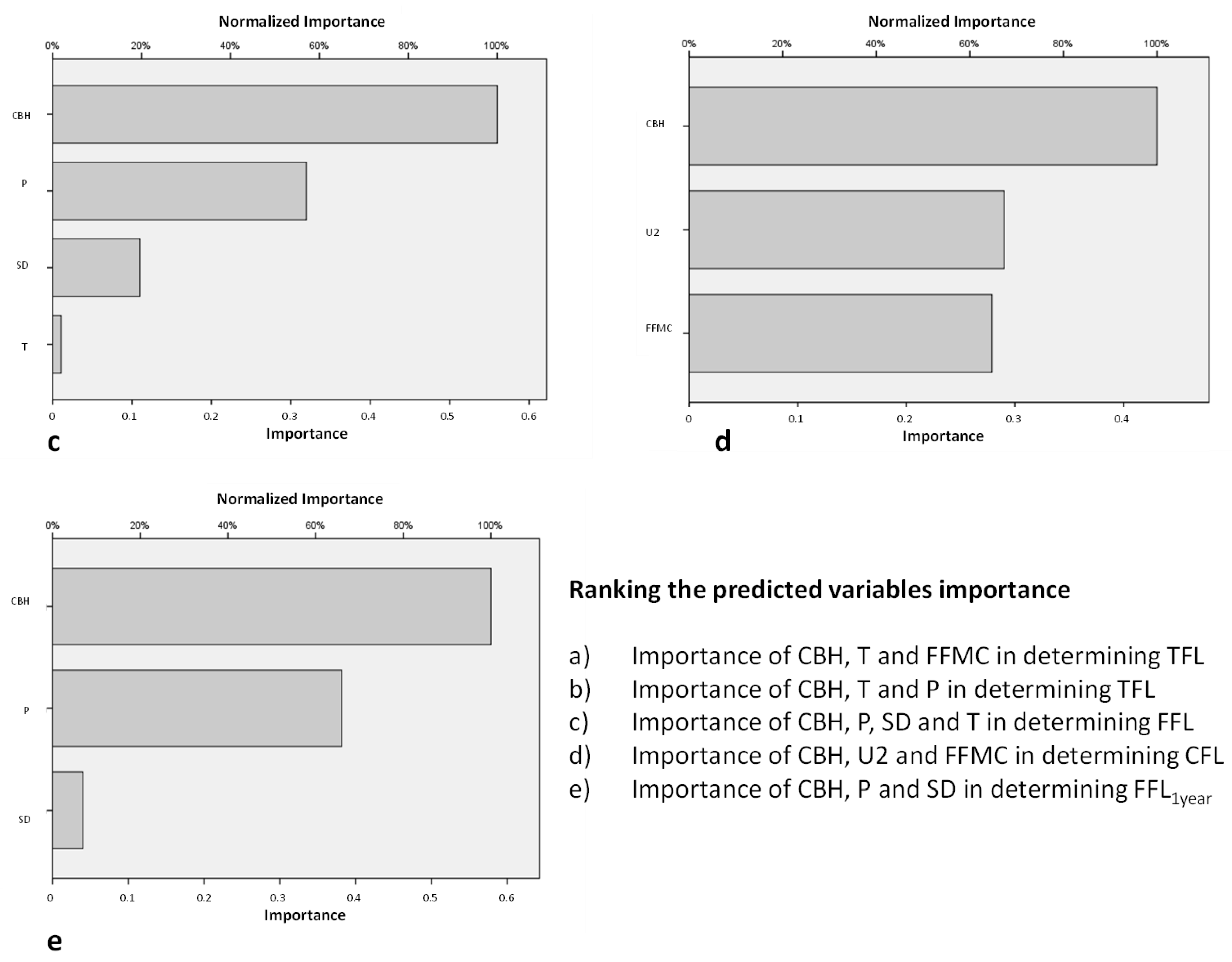
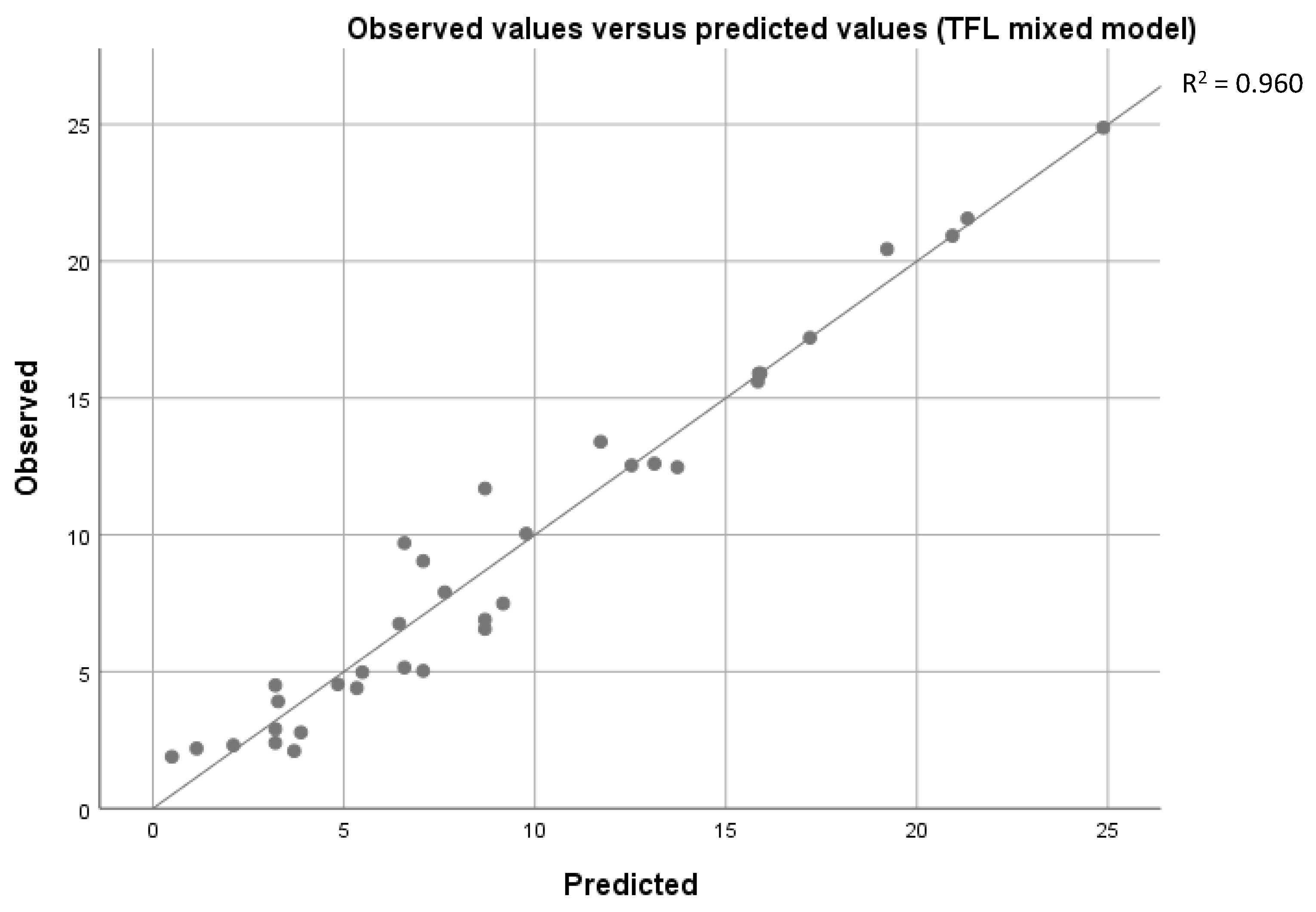
The mixed model using CBH, T, and P was the most reliable predictor of TFL for our prescribed fires (
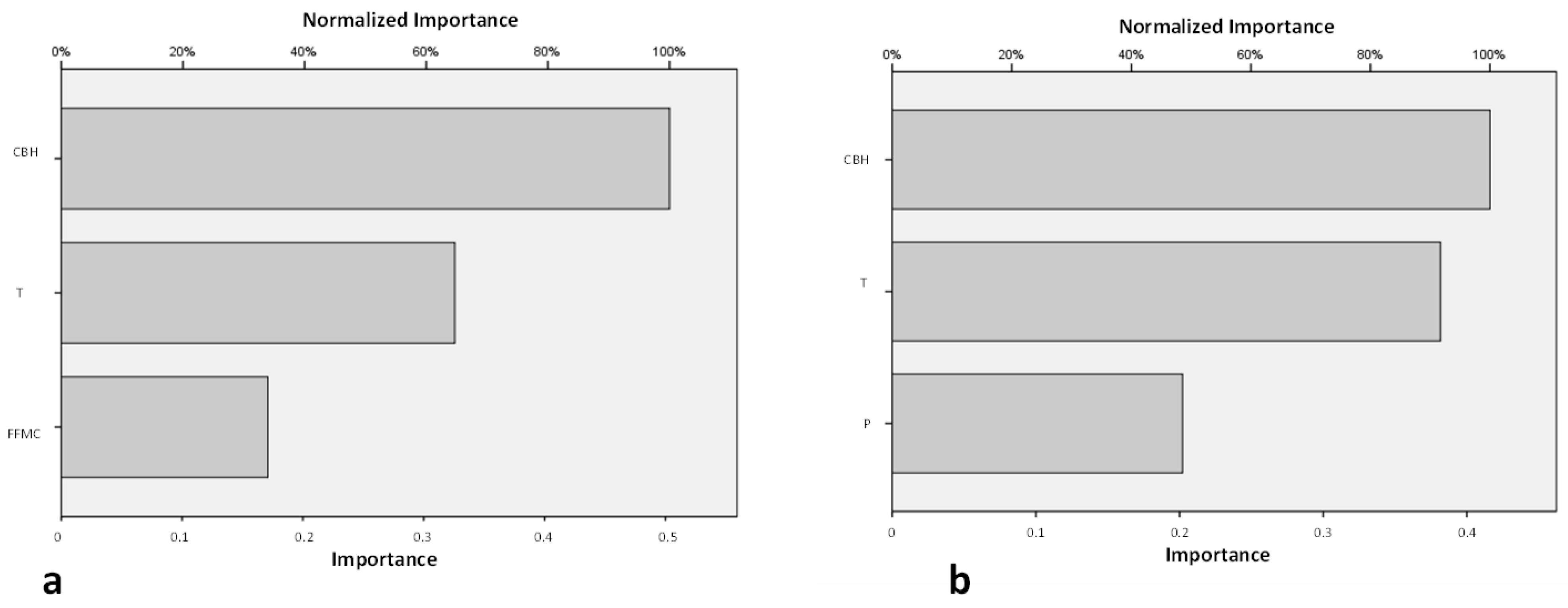
Figure 8). This approach also includes six multiexponential models that could be of great value in useful-life identification, according to their simplicity and continuous scale. TFL dynamics is associated with stand variables, burning implementation conditions, and postburn meteorological characteristics. In this sense, the TFL dynamics model depends mainly on CBH, T, P, and FFMC (Figure 4). All these variables were positively related; therefore, higher TFL is associated with a higher value of independent variables, except for CBH. The T and CBH values have already been identified as keystone factors in postburn fuel evolution [8,13,16]. A lower CBH value is related to higher TFL due to thermal pruning effects. FFMC has already been established as an essential factor in the burn windows for P. pinaster in Sierra Morena [22]. A high volume of P influences the fuel load because of greater twig and branch elongation and a greater amount of new needle generation than in dry years [42]. Not only do scorched needles fall on the ground, old branches, live needles, twigs, and the lowest branches, due to the light competence, will also fall. Other studies [43,44] have shown that heavy precipitation can promote more notable effects in the amount of fuel beneath a forest canopy, mainly in stands with a low basal area. In this sense, our study stands were characterized by a low basal area, ranging from 9.6 (Viso D) to 31.13 m2/ha (Puebla A). This low basal area could have emphasized the relative importance of postburn precipitation in our findings. Finally, a greater FFMC value during burning implementation is associated with a high TFL value due to the low FC.
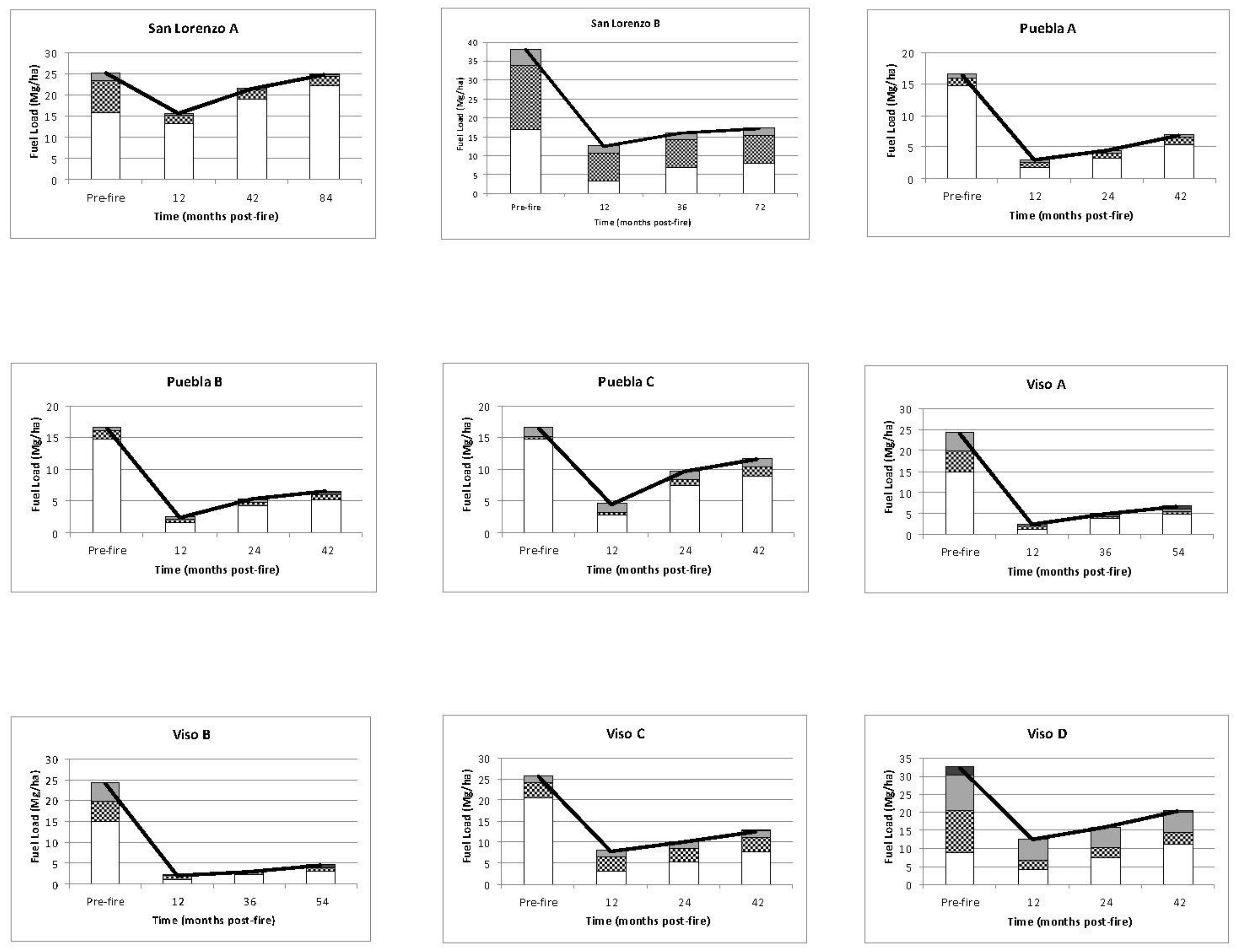
TFL postfire reduction for our sampling plots (with the thermal pruning already incorporated) ranged from 38.14% (San Lorenzo A) to 92.18% (Viso B). This TFL reduction is directly related to FFMC. In this sense, an FFMC value lower than 9% was associated with an average TFL of 79.91%, FFMC values higher than 9% and less than 12%, with an average of 91.31%, FFMC values higher than 12% and less than 14%, with an average of 77.54%, and FFMC values higher than 14%, with an average of 38.14%. Although [22] showed that burn windows would require FFM values from 9% to 15%, this approach only considered FFL consumption immediately postfire, without thermal pruning effects. The prescribed fire targets would be achieved with FFMC ranging from 9% to 12%, according to our findings and TFL reduction above 80%, which is generally established in the burn windows of the study area. If there is a high amount of 10- and 100-h time-lag fuels (>10 Mg/ha), TFL will be considerably reduced (64.19%). In these specific cases, a TFL reduction of 80% cannot be reached by a single burning as it could damage the trees. If a reduction target of 65% of TFL is established in these stands, we would prescribe a burn with FFMC ranging from 10.5% to 12%, using spot-heading fire to reduce the I value.
FFL dynamics is directly related to CBH, P, SD, and T (Figure 4). In a similar way to TFL, a lower CBH value and a higher T value are associated with higher FFL. Reference [20] indicated that the postburn fuel load is greater in lower-height stands due to higher thermal pruning. Similarly, higher SD is related to higher FFL because of the higher amount of fallen needles due to thermal pruning. With similar TFL values, a higher P value was associated with higher FFL due to a large amount of fallen needles and twigs [43]. Regarding this fall, some studies [45] have linked precipitation and the amount of annual fallen needles. The FFL evolution from the first year depends on CBH, SD, and P. Reference [46] found a bigger number of needles during the first postburn months, which seems to corroborate this model for the first year.
CFL depends on CBH, U2, and FFMC (Figure 4). In a similar way to TFL and FFL, a lower CBH value and a higher FFMC value was associated with higher CFL. Some authors [20] have pointed out that higher postfire CFL is based on needles and twigs that have fallen from the forest canopy and the suppressed tree mortality. Higher FFMC is related to lower coarse fuel consumption [22]. High CFL corresponds to low U2 and, consequently, a lower I value, which promotes much lower coarse fuel consumption [22]. Generally, the FC differences in these fuel model types are associated with coarse fuel consumption, given the elevated level of fine fuel consumption [3].
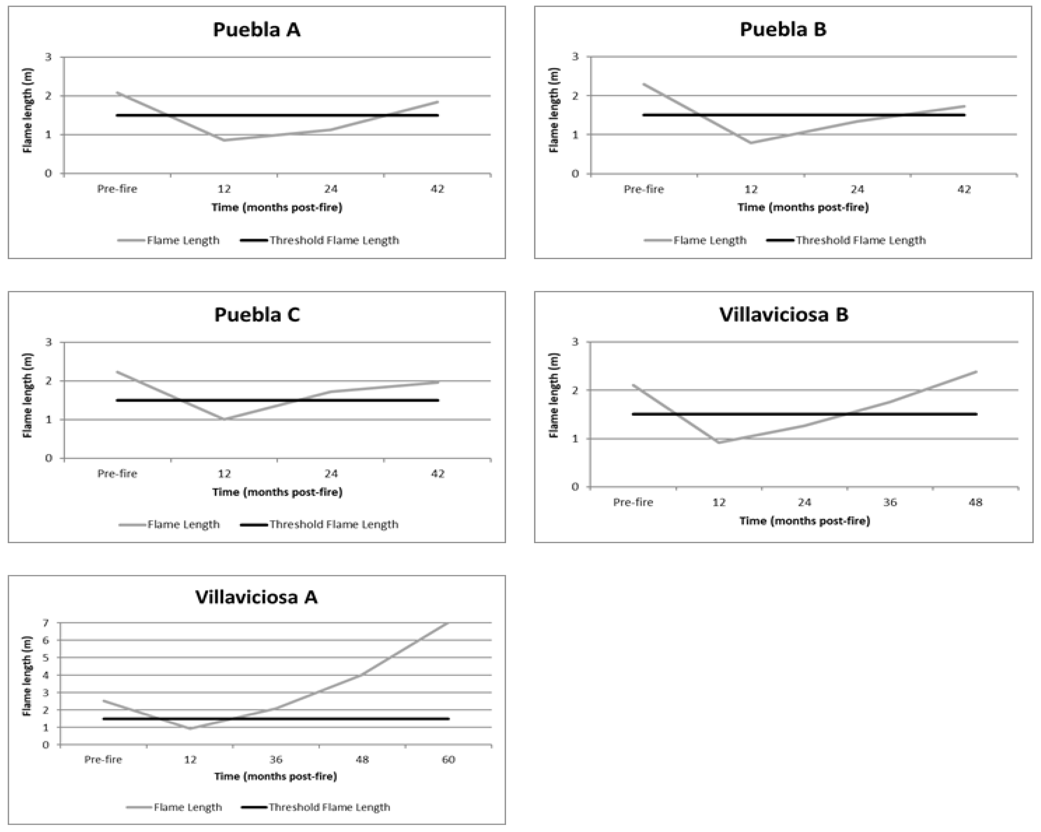
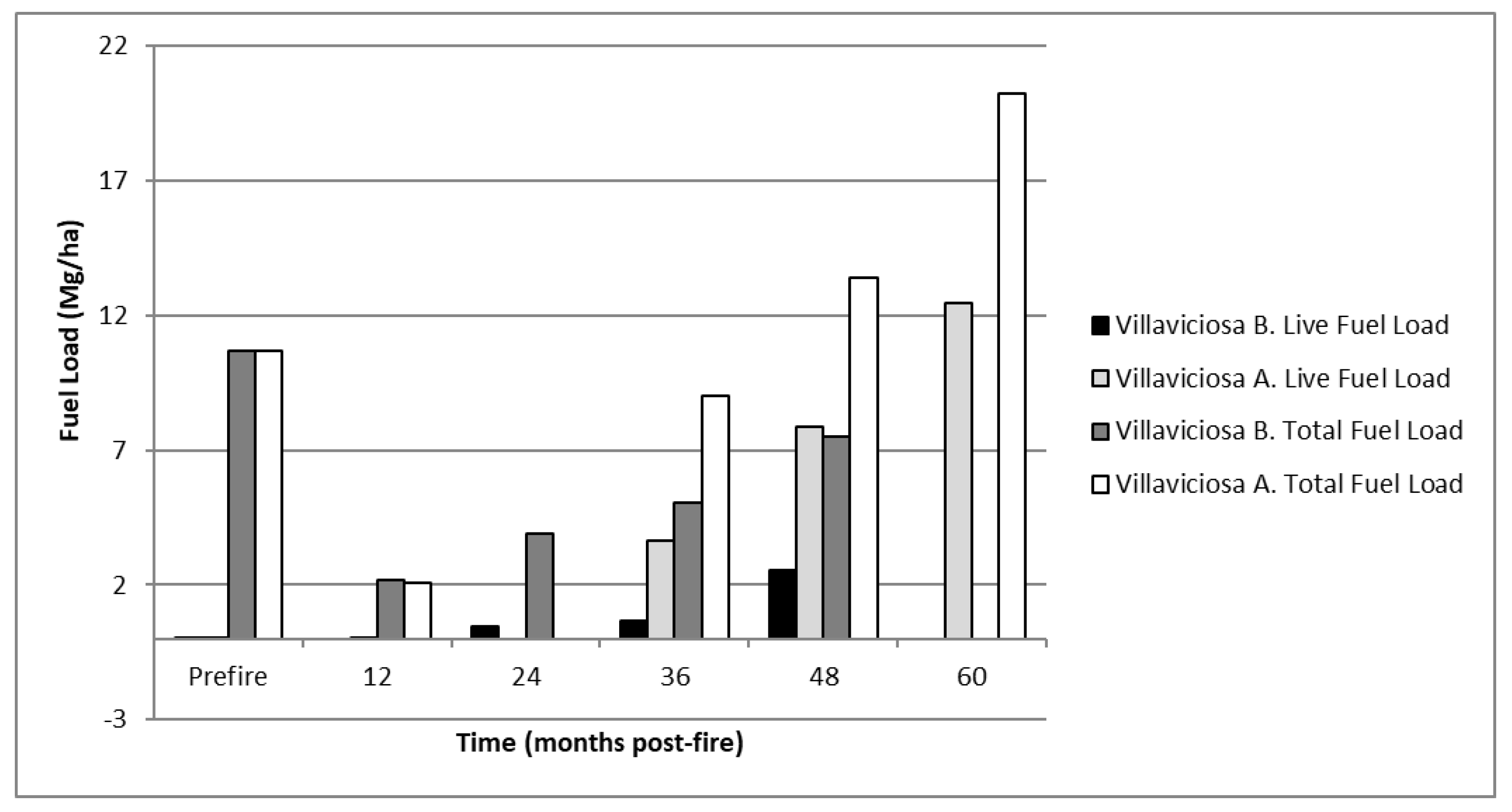
LFL dynamics from the second year depend to a large extent on CC. LFL was increased mainly from the second year for stands with low CC. This is mainly explained by the high gap colonization of the dominant understory species (C. ladanifer) because of its wide seed bank and its high germination percentage after its exposure to a heat source [23,25]. Many differences between Villaviciosa A and Villaviciosa B were observed (Figure 9) due to their CC difference (Table 2). The inventory carried out after 36 months and 48 months showed a difference of 82.14% and 67.89%, respectively, in the LFL evolution between them. The time elapsed from the burning reduced the effective difference due to fuel dynamics. According to the periodical inventories of the 11 prescribed fires, LFL was not generated after four years with stands where CC was over 75%. With CC values lower than 75%, LFL was generated between the second and the third year. The fuel model was converted from litter-slash fuel to litter-slash-understory, mainly from the third year, for stands where their CC values were under 50%. This fuel modification promotes an increase in FL, which should be considered in the useful life of the prescribed fire. Regarding stands with CC values lower than 50%, suppression difficulties could be found using direct attack with hand tools under the 95% percentile scenario [32]. Therefore, the traditional burn windows used by fire agencies of the study areas usually established an upper threshold of 1.5 m in FL. Consequent to the TFL dynamic, the burn windows would be limited from the fourth year onward in P. pinaster stands where CC is lower than 50%, not reaching the expected results of TFL consumption.
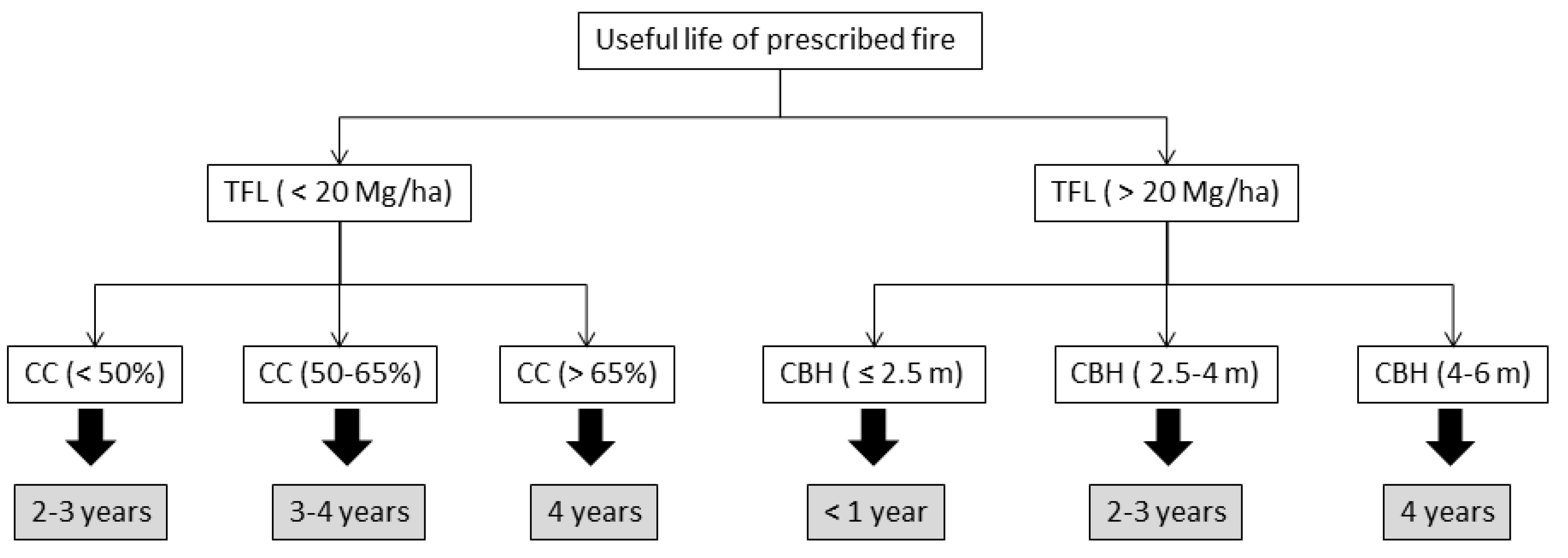
A tree decision tool for the maritime pine stands of Sierra Morena (Figure 10) was built based on fuel load dynamics (Groups I to V) and its useful life (Groups A to D). Two preburn fuel models were established according to the biomass harvesting slash: <20 Mg/ha (full tree harvesting system and tree forwarding) and >20 Mg/ha (cut-to-length logging system and tree skidding). Once the prescribed fire is implemented, useful life depends on CC. With CC values lower than 50% (Group III-A), the burning is only effective for 2–3 years due to the high colonization of C. ladanifer. This effective rotation length is in line with [47] in Canada and [16] in maritime pine stands in the south of Europe. With CC values between 50% and 65%, the useful life is increased by up to 3–4 years. With over 65% in CC values, prescribed fire effectiveness is at least 4 years (Groups I-B and II-B), similar to previous research [8,19,20,21,42,
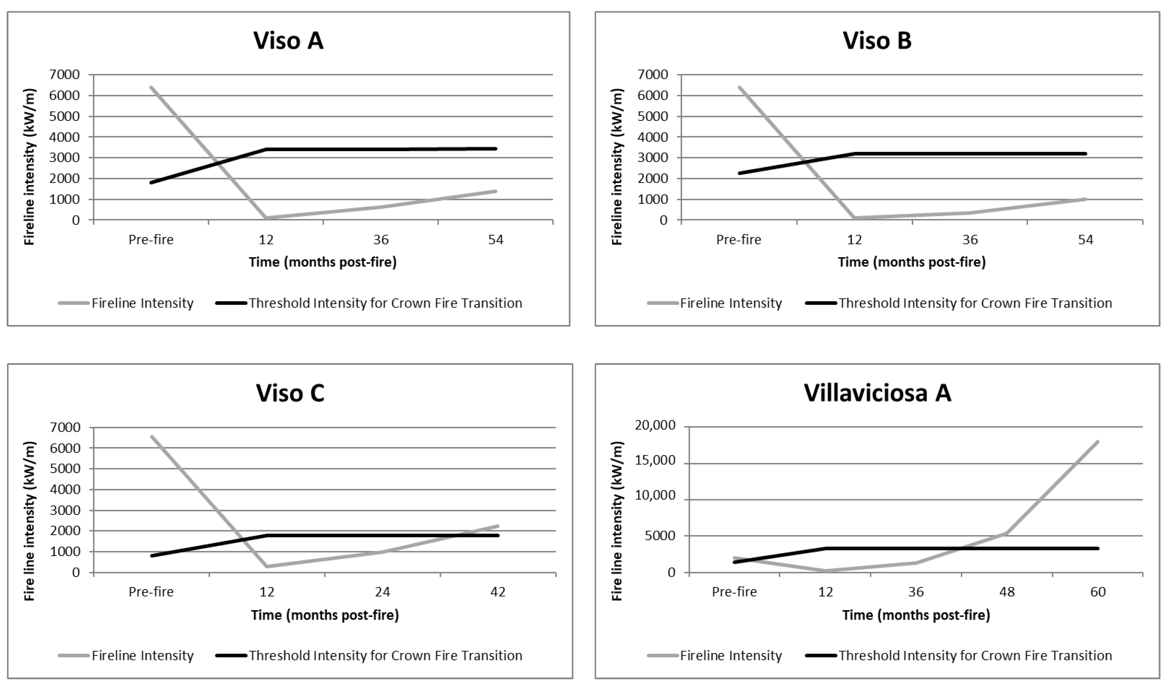
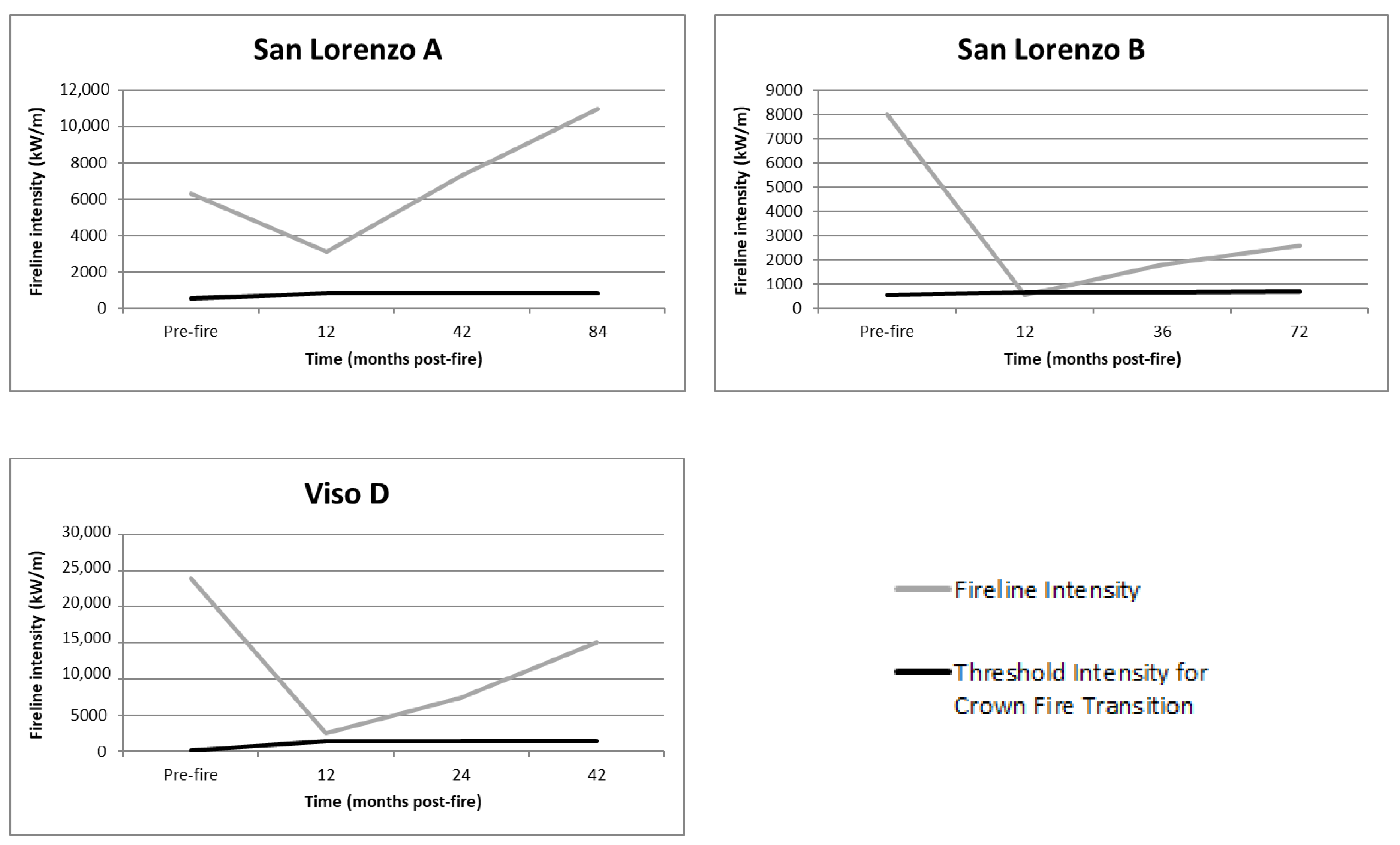
48]. The prescribed fires with TFL higher than 20 Mg/ha have shown uneven results (Figure 8). In the case of stands with less than 2.5 m CBH (Groups IV-D and V-D), the burning did not achieve the mitigation of the threshold for transition from surface fire to crown fire. These stands required a second prescribed fire in the following 1 or 2 years to reach fuel treatment effectiveness. Between 2.5 and 4 m CBH (Group II-A), the useful life of the prescribed fire is increased by up to 2–3 years according to FFMC. Finally, with more than 4 m CBH (Group I-A), the useful life of the prescribed fire rises to at least 4 years, similar to other studies [8,20].
Prescribed fires are an interesting silvicultural treatment for fire behavior mitigation and, therefore, for forest fire hazard reduction [9,10,42]. According to our useful-life findings, prescribed fires have been identified as a very effective prevention tool for maritime pine stands with TFL values over 20 Mg/ha and CBH values higher than 2.6 m, mainly in stands with CBH values higher than 4 m. The monitoring and methodological framework to useful-life identification can be extrapolated to any territory and spatial scale; only periodical field inventories and fire behavior simulations would be needed. The very efficient use of prescribed fire is required according to its uncertainty of use perspective [5,6,11], budget constraints [16], and meteorological or burn window limitations [22]. Further studies are encouraged to evaluate the effects of repeated prescribed fires [8] in stands with TFL values higher than 20 Mg/ha and CBH values lower than 2.5 m. Similarly, a comparative analysis of postburn fuel dynamics and the useful life of prescribed fire, according to different season implementation [3], would be encouraged. Nevertheless, the study area managers consider spring to be the best season for prescribed fire implementation due to the low availability of fuel in autumn and winter, according to precipitation and local fog. In summer, regional governments of the study areas prohibit the implementation of prescribed fires.
The combinative implementation of thinning for biomass harvesting and prescribed fire for fuel load maintenance is an interesting opportunity for P. pinaster management of stands in the Mediterranean Basin. On the one hand, thinning provides an economic benefit and reduces the ROS value in a crown fire [4,49]. Thinning is also a tool to increase the resistance and resilience of forests [50] to climate change in the southern Iberian Peninsula [51]. The lower SD would reduce tree competence, mainly in periods of extreme drought [52]. On the other hand, prescribed fire implementation would regularly reduce TFL, pointing to fire intensity reduction for the transition from surface fire to crown fire [38], the severity of forest fire [14], suppression difficulty [31], and socioeconomic impacts and suppression costs [2]. P. pinaster has a high resistance to low and moderate prescribed fire intensities [18]. Therefore, it would not present any problems from the point of view of ecological impact or tree mortality [16]. Furthermore, prescribed burning is a much cheaper fuel treatment than mechanical treatments [53], showing no differences between them after the fourth year in dominated Cistus spp. ecosystems [25]. Finally, it should be noted that prescribed fire use implies an advantage over other forest treatments from the point of view of firefighter training [22].

5. Conclusions

Prescribed fires are considered an effective tool for fire severity reduction and the mitigation of critical surface intensity for the transition from surface fire to crown fire. The postburn fuel dynamics or evolution depends not only on time elapsed from the burning but also on fine fuel moisture content and fuel availability during the burning implementation. Canopy base height and canopy closure also have a great influence on the amount of fallen needles and twigs and the colonization of live fuel. Therefore, the useful life of prescribed fires, in a similar way to other silvicultural treatments, is limited, ranging from 0 to 4 years from P. pinaster stands in southern Europe.
The thinning implementation and further surface fuel maintenance using prescribed fires emphasize the reduction of forest fire hazards. Nevertheless, it has been justified that heavy thinning causes low canopy closure and, consequently, the substantial reduction of the useful life of the treatment. According to stand characteristics, the manager should decide on the fuel moisture content in the burn window to maximize the useful life of the treatment. The helpfulness of a fuel dynamics model based on burning condition implementation is of huge interest to forest managers. However, the prescribed fire implementation is very limited according to the difficulty of administrative authorizations, meteorological condition limitations, the presence of settlements, and ecological constraints. Therefore, prescribed fires should constitute an additional tool to complement mechanical fuel treatments.

Author Contributions

J.R.M. contributed to the methodology, formal analysis, data curation, and original draft preparation; M.O. participated in conceptualization, data curation, and writing—review and editing; F.R.yS. contributed to the methodology, formal analysis, supervision, and funding acquisition. All authors have read and agreed to the published version of the manuscript.

Funding

This research was funded by the National Institute for Agricultural Research (INIA) of the Spanish Ministry of Science, Innovation, and Universities, cofounded by FEDER funds (VIS4FIREproject, RTA2017-00042-C05-01) and the CILIFO project from the European Union (INTERREG-POCTEP 0753_CILIFO_5_E).

Data Availability Statement

Data available on request.

Acknowledgments

The authors of this study would like to express their gratitude to all the technicians and teams that have contributed to the data used in this study. The authors thank two anonymous reviewers and the editor for their help in improving the presentation and content of this manuscript.

Conflicts of Interest

The authors declare no conflict of interest.

Appendix A

Table A1. Area and number of sampling plots and destructive sampling units for each prescribed fire.
BurningDateArea (ha)Sampling Plots (1000 m2)Destructive Sampling Units (1 m2)
San Lorenzo A20104.1927
San Lorenzo B20112.5618
Puebla A20144.8618
Puebla B20142.8416
Puebla C20141.8416
Viso A20152.9824
Viso B20153.1618
Viso C20161.2416
Viso D20163.2416
Villaviciosa A20151.1416
Villaviciosa B20161.6416

Appendix B

Table A2. Estimation of fire behavior parameters based on weather scenarios and periodical vegetation dynamics.
Prescribed FirePostburn Time (Months)Spread Rate (m/min)Heat per Unit Area (kJ/m2)Fire-Line Intensity (kW/m)Flame Length (m)Threshold Intensity for Crown Fire Transition (kW/m)
San Lorenzo APreburn8.146,6576298.704.33553.80
San Lorenzo A126.528,8603126.503.14804.35
San Lorenzo A421139,8867312.434.64842.61
San Lorenzo A8414.346,02810,970.015.59838.33
San Lorenzo BPreburn7.762,4938019.944.84542.66
San Lorenzo B121.423,199541.311.40645.56
San Lorenzo B363.729,4151813,932.44641.65
San Lorenzo B724.931,8202598.632.88677.18
Puebla APreburn2.530,691.51278.812.082340.98
Puebla A122.15365187.780.864475.16
Puebla A242.58140339.171.134475.16
Puebla A424.612,765978.651.844538.85
Puebla BPreburn3.130,691.51585.732.302340.98
Puebla B122.14440155.400.794106.65
Puebla B2439860.5493.031.344106.65
Puebla B424.212,136849.521.724168.55
Puebla CPreburn2.930,691.51483.422.232340.98
Puebla C121.98325263.631.014103.02
Puebla C242.817,945837.431.714099.39
Puebla C423.121,626.51117.371.964088.51
Viso APreburn8.644,7336411.734.371820.39
Viso A121.64310.5114.950.693402.10
Viso A3649213614.201.493398.69
Viso A546.612,487.51373.632.153449.96
Viso BPreburn8.644,7336411.734.372251.21
Viso B121.63496.593.240.623202.83
Viso B364.25143360.011.163199.49
Viso B547.383991021.881.883179.46
Viso CPreburn8.347,4716566.824.42812.80
Viso C121.214,615292.301.061781.76
Viso C243.218,574990.611.851776.26
Viso C425.823,3102253.302.701773.52
Viso DPreburn2459,75523,902.008.01141.99
Viso D126.523,069.52499.202.831431.42
Viso D2415.129,4157402.784.671431.42
Viso D4223.937,81415,062.586.471380.61
Villaviciosa APreburn619,7581975.802.541416.11
Villaviciosa A123.53885226.630.943259.84
Villaviciosa A364.716,7241310.052.113259.84
Villaviciosa A481324,7905371.174.033246.39
Villaviciosa A6028.937,425.518,026.627.033212.87
Villaviciosa BPreburn419,7581317.22.111571.65
Villaviciosa B123.24051.5216.080.922749.55
Villaviciosa B243.67233.5434.011.272740.02
Villaviciosa B365.79305.5884.021.762730.51
Villaviciosa B487.413,856.51708.972.382717.83

References

  1. Moreira, F.; Viedma, O.; Arianoutsou, M.; Curt, T.; Koutsias, N.; Rigolot, E.; Barbati, A.; Corona, P.; Vaz, P.; Xanthopoulos, G.; et al. Landscape–wildfire interactions in southern Europe: Implications for landscape management. J. Environ. Manag. 2011, 92, 2389–2402. [Google Scholar] [CrossRef] [Green Version]
  2. Molina, J.R.; González-Cabán, A.; Silva, F.R.Y. Potential Effects of Climate Change on Fire Behavior, Economic Susceptibility and Suppression Costs in Mediterranean Ecosystems: Córdoba Province, Spain. Forests 2019, 10, 679. [Google Scholar] [CrossRef] [Green Version]
  3. Knapp, E.E.; Keeley, J.E.; Ballenger, E.A.; Brennan, T.J. Fuel reduction and coarse woody debris dynamics with early season and late season prescribed fire in a Sierra Nevada mixed conifer forest. For. Ecol. Manag. 2005, 208, 383–397. [Google Scholar] [CrossRef]
  4. Agee, J.K.; Skinner, C.N. Basic principles of forest fuel reduction treatments. For. Ecol. Manag. 2005, 211, 83–96. [Google Scholar] [CrossRef]
  5. Ryan, K.C.; Knapp, E.E.; Varner, J.M. Prescribed fire in North American forests and woodlands: History, current practice, and challenges. Front. Ecol. Environ. 2013, 11, 15. [Google Scholar] [CrossRef]
  6. Valor, T.; González-Olabarria, J.R.; Piqué, M. Assessing the impact of prescribed burning on the growth of European pines. For. Ecol. Manag. 2015, 343, 101–109. [Google Scholar] [CrossRef]
  7. Knapp, E.E.; Varner, J.M.; Busse, M.D.; Skinner, C.N.; Shestak, C.J. Behaviour and effects of prescribed fire in masticated fuelbeds. Int. J. Wildland Fire 2011, 20, 932–945. [Google Scholar] [CrossRef]
  8. Stephens, S.L.; McIver, J.D.; Boerner, R.E.J.; Fettig, C.J.; Fontaine, J.B.; Hartsough, B.R.; Kennedy, P.L.; Schwilk, D.W. The Effects of Forest Fuel-Reduction Treatments in the United States. BioScience 2012, 62, 549–560. [Google Scholar] [CrossRef] [Green Version]
  9. McCaw, W.L. Managing forest fuels using prescribed fire–A perspective from southern Australia. For. Ecol. Manag. 2013, 294, 217–224. [Google Scholar] [CrossRef]
  10. Piqué, M.; Domènech, R. Effectiveness of mechanical thinning and prescribed burning on fire behavior in Pinus nigra forests in NE Spain. Sci. Total Environ. 2018, 618, 1539–1546. [Google Scholar] [CrossRef]
  11. Fernandes, P.M.; Davies, G.M.; Ascoli, D.; Fernández, C.; Moreira, F.; Rigolot, E.; Stoof, C.R.; Vega, J.A.; Molina, D. Prescribed burning in southern Europe: Developing fire management in a dynamic landscape. Front. Ecol. Environ. 2013, 11, 4. [Google Scholar] [CrossRef] [Green Version]
  12. Fernandes, P.M. Empirical Support for the Use of Prescribed Burning as a Fuel Treatment. Curr. For. Rep. 2015, 1, 118–127. [Google Scholar] [CrossRef] [Green Version]
  13. Brose, P.; Wade, D. Potential fire behavior in pine flatwood forests following three different fuel reduction techniques. For. Ecol. Manag. 2002, 163, 71–84. [Google Scholar] [CrossRef]
  14. Coppoletta, M.; Merriam, K.E.; Collins, B.M. Post- fire vegetation and fuel development influences fire severity patterns in reburns. Ecol. Appl. 2016, 26, 686–699. [Google Scholar] [CrossRef] [PubMed]
  15. Peterson, D.W.; Reich, P.B. Prescribed fire in oak savanna: Fire frequency effects on stand structure and dynamics. Ecol. Appl. 2001, 11, 914–927. [Google Scholar] [CrossRef]
  16. Fernandes, P.M.; Botelho, H.S. A review of prescribed burning effectiveness in fire hazard reduction. Int. J. Wildland Fire 2003, 12, 117–128. [Google Scholar] [CrossRef] [Green Version]
  17. Fernandes, P.M.; Rigolot, E. The fire ecology and management of maritime pine (Pinus pinaster Ait.). For. Ecol. Manag. 2007, 241, 1–13. [Google Scholar] [CrossRef]
  18. Fernandes, P.M.; Vega, J.A.; Jiménez, E.; Rigolot, E. Fire resistance of European pines. For. Ecol. Manag. 2008, 256, 246–255. [Google Scholar] [CrossRef]
  19. Peterson, D.; Sackett, S.; Robinson, L.; Haase, S. The Effects of Repeated Prescribed Burning on Pinus ponderosa Growth. Int. J. Wildland Fire 1994, 4, 239–247. [Google Scholar] [CrossRef] [Green Version]
  20. Van Mantgem, P.J.; Lalemand, L.B.; Keifer, M.; Kane, J.M. Duration of fuels reduction following prescribed fire in coniferous forests of U.S. national parks in California and the Colorado Plateau. For. Ecol. Manag. 2016, 379, 265–272. [Google Scholar] [CrossRef]
  21. Pollet, J.; Omi, P.N. Effect of thinning and prescribed burning on crown fire severity in ponderosa pine forests. Int. J. Wildland Fire 2002, 11, 1–10. [Google Scholar] [CrossRef]
  22. Molina, J.R.; García, J.P.; Fernández, J.J.; Silva, F.R.Y. Prescribed fire experiences on crop residue removal for biomass exploitations. Application to the maritime pine forests in the Mediterranean Basin. Sci. Total Environ. 2018, 612, 63–70. [Google Scholar] [CrossRef] [PubMed]
  23. Valbuena, L.; Tarrega, R.; Luis, E. Influence of Heat on Seed Germination of Cistus laurifolius and Cistus ladanifer. Int. J. Wildland Fire 1992, 2, 15–20. [Google Scholar] [CrossRef]
  24. Potts, J.B.; Marino, E.; Stephens, S.L. Chaparral shrub recovery after fuel reduction: A comparison of prescribed fire and mastication techniques. Plant Ecol. 2010, 210, 303–315. [Google Scholar] [CrossRef] [Green Version]
  25. Tárrega, R.; Luis-Calabuig, E.; Valbuena, L. Eleven years of recovery dynamic after experimental burning and cutting in two Cistus communities. Acta Oecologica 2001, 22, 277–283. [Google Scholar] [CrossRef]
  26. Anderson, H.E. Aids to Determining Fuel Models for Estimating Fire Behavior; USDA Forest Service: Boise, ID, USA, 1982; p. 22.
  27. Scott, J.H.; Burgan, R.E. Standard fire behaviour fuel model: A comprehensive set for use with Rothermel’s surface fire spread model. In General Technical Report RMRS-GTR-153; USDA Forest Service: Boise, ID, USA, 2005; p. 72. [Google Scholar]
  28. Rodríguez y Silva, F.; Molina, J.R. Modeling Mediterranean forest fuels by integrating field data and mapping tools. Eur. J. For. Res. 2012, 131, 571–582. [Google Scholar] [CrossRef]
  29. Regional Government of Andalusia. Manual de Ordenación de Montes de Andalucía; Junta de Andalucía: Sevilla, Spain, 2004; p. 356.
  30. Stephens, S.L.; Moghaddas, J.J. Experimental fuel treatment impacts on forest structure, potential fire behavior, and predicted tree mortality in a California mixed conifer forest. For. Ecol. Manag. 2005, 215, 21–36. [Google Scholar] [CrossRef]
  31. Silva, F.R.Y.; O’Connor, C.D.; Thompson, M.P.; Martínez, J.R.M.; Calkin, D.E. Modelling suppression difficulty: Current and future applications. Int. J. Wildland Fire 2020, 29, 739. [Google Scholar] [CrossRef]
  32. Andrews, P.L.; Rothermel, R.C. Charts for Interpreting Wildland Fire Behavior Characteristics; USDA Forest Service: Boise, ID, USA, 1982; p. 21.
  33. Andrews, P.L.; Bevins, C.D.; Seli, R.C. BehavePlus fire modeling system, version 2.0: User’s guide. In General Technical Report RMRS-GTR-106WWW; USDA Forest Service: Boise, ID, USA, 2003; p. 132. [Google Scholar]
  34. Finney, A.M. Fire growth using minimum travel time methods. Can. J. For. Res. 2002, 32, 1420–1424. [Google Scholar] [CrossRef]
  35. Fernandes, P.M.; Loureiro, C.; Botelho, H. PiroPinus: A spreadsheet application to guide prescribed burning operations in maritime pine forest. Comput. Electron. Agric. 2012, 81, 58–61. [Google Scholar] [CrossRef] [Green Version]
  36. Rothermel, R.C. A mathematical model for predicting fire spread in wildland fires. In Research Paper INT-115.Department of Agriculture, Forest Service; Intermountain Forest and Range Experiment Station: Ogden, UT, USA, 1972. [Google Scholar]
  37. Byram, G.M. Combustion of forest fuels. In Forest Fire: Control and Use; Davis, K.P., Ed.; McGraw-Hill: New York, UY, USA, 1959; pp. 61–89, 554–555. [Google Scholar]
  38. Van Wagner, C.E. Conditions for the start and spread of crown fire. Can. J. For. Res. 1977, 7, 23–34. [Google Scholar] [CrossRef]
  39. Agroclimatic Information System for Irrigation (SIAR). Available online: http://eportal.mapa.gob.es (accessed on 14 November 2020).
  40. Cardil, A.; Molina, D.M.; Kobziar, L.N. Extreme temperature days and their potential impacts on southern Europe. Nat. Hazards Earth Syst. Sci. 2014, 14, 3005–3014. [Google Scholar] [CrossRef] [Green Version]
  41. Molina, J.R.; Rodríguez y Silva, F.; Herrera, M.A. Potential crown fire behaviour in Pinus pinea stands following different fuel treatments. For. Syst. 2011, 20, 266–277. [Google Scholar]
  42. Irvine, J.; Perks, M.P.; Magnani, F.; Grace, J. The response of Pinus sylvestris to drought: Stomatal control of transpiration and hydraulic conductance. Tree Physiol. 1998, 18, 393–402. [Google Scholar] [CrossRef]
  43. Schlesinger, W.H.; Dietze, M.C.; Jackson, R.B.; Phillips, R.P.; Rhoades, C.C.; Rustad, L.E.; Vose, J.M. Forest biogeochemistry in response to drought. Glob. Chang. Biol. 2015, 22, 2318–2328. [Google Scholar] [CrossRef]
  44. Espinosa, J.; Rodríguez De Rivera, Ó.; Madrigal, J.; Guijarro, M.; Hernando, C. Use of Bayesian Modeling to Determine the Effects of Meteorological Conditions, Prescribed Burn Season, and Tree Characteristics on Litterfall of Pinus nigra and Pinus pinaster Stands. Forests 2020, 11, 1006. [Google Scholar] [CrossRef]
  45. Santa Regina, I.; Gallardo, J.F. Producción de hojarasca en tres bosques de la Sierra de Béjar (Salamanca). Mediterr. Ser. Biol. 1985, 8, 89–101. [Google Scholar] [CrossRef] [Green Version]
  46. Espinosa, J.; Madrigal, J.; De La Cruz, A.; Guijarro, M.; Jimenez, E.; Hernando, C. Short-term effects of prescribed burning on litterfall biomass in mixed stands of Pinus nigra and Pinus pinaster and pure stands of Pinus nigra in the Cuenca Mountains (Central-Eastern Spain). Sci. Total Environ. 2018, 618, 941–951. [Google Scholar] [CrossRef]
  47. McCarthy, G.L.; Tolhurst, K.G. Effectiveness of broadscale fuel reduction burning in assisting with wildfire control in parks and forests in Victoria. In Natural Resources and Environment 2001, Research Report No 51; Department of Natural Resources and Environment Melbourne: Melbourne, Victoria, Australia, 2001. [Google Scholar]
  48. Lydersen, J.M.; North, M.P.; Collins, B.M. Severity of an uncharacteristically large wildfire, the Rim Fire, in forests with relatively restored frequent fire regimes. For. Ecol. Manag. 2014, 328, 326–334. [Google Scholar] [CrossRef] [Green Version]
  49. Cruz, M.G.E.; Alexander, M.; Wakimoto, R.H. Development and testing of models for predicting crown fire rate of spread in conifer forest stands. Can. J. For. Res. 2005, 35, 1626–1639. [Google Scholar] [CrossRef]
  50. Derose, R.J.; Long, J.N. Resistance and Resilience: A Conceptual Framework for Silviculture. For. Sci. 2014, 60, 1205–1212. [Google Scholar] [CrossRef]
  51. Duque, J.; Navarro, R.; Sánchez-Salguero, R.; Rodríguez, C. Is thinning an alternative when trees could die in response to drought? The case of planted Pinus nigra and P. Sylvestris stands in southern Spain. For. Ecol. Manag. 2019, 433, 313–324. [Google Scholar]
  52. Van Mantgem, P.J.; Caprio, A.C.; Stephenson, N.L.; Das, A.J. Does Prescribed Fire Promote Resistance to Drought in Low Elevation Forests of the Sierra Nevada, California, USA? Fire Ecol. 2016, 12, 13–25. [Google Scholar] [CrossRef]
  53. Hartsough, B.R.; Abrams, S.; Barbour, R.J.; Drews, E.S.; McIver, J.D.; Moghaddas, J.J.; Schwilk, D.W.; Stephens, S.L. The economics of alternative fuel reduction treatments in western United States dry forests: Financial and policy implications from the National Fire and Fire Surrogate Study. For. Policy Econ. 2008, 10, 344–354. [Google Scholar] [CrossRef]
Figure 1. Study area location (shaded areas correspond to the two provinces, Córdoba and Ciudad Real).
Forests 12 00486 g001
Figure 2. Temporal dynamics of the fuel load by categories in each stand.
Forests 12 00486 g002
Figure 3. Agglomerative cluster analysis based on the Ward method.
Forests 12 00486 g003
Figure 4. Ranking of the predicted variables’ importance based on an artificial neural network.
Forests 12 00486 g004aForests 12 00486 g004b
Figure 5. Fire-line intensity versus threshold intensity for crown fire transition in Groups A (Viso A, Viso B, Viso C) and C (Villaviciosa A). If the fire intensity is higher than threshold intensity, surface fire will be sufficient to ignite tree crowns.
Forests 12 00486 g005
Figure 6. Evolution of flame length in Groups B (Puebla A, Puebla B, Puebla C, Villaviciosa B) and C (Villaviciosa A). A flame length threshold (1.5 m) was established by a direct firefighting attack with hand tools.
Forests 12 00486 g006
Figure 7. Fire-line intensity versus threshold intensity for crown fire transition in Group D (San Lorenzo A, San Lorenzo B, and Viso D). If the fire intensity is higher than threshold intensity, surface fire will be sufficient to ignite tree crowns.
Forests 12 00486 g007
Figure 8. Plots of observed versus predicted values of TFL dynamics using the mixed model.
Forests 12 00486 g008
Figure 9. Dynamics of total fuel load and live fuel load in Villaviciosa A and Villaviciosa B.
Forests 12 00486 g009
Figure 10. Decision tree for the estimation of the useful life of a prescribed fire. “TFL” is the total preburn fuel load (Mg/ha); “CC” is the canopy cover (%); “CBH” is the canopy base height (m).
Forests 12 00486 g010
Table 1. Characterization of environmental conditions, flame length, and fire pattern for each stand.
Prescribed FireSeasonFine Fuel Moisture (%)Mean Wind Speed (km/h) *Flame Length (m)Fire Ignition Pattern
San Lorenzo ASpring13.5–14.55–70.4–0.8Strip-heading fire
San Lorenzo BSpring10.5–11.51–30.9–1.2Spot-heading fire
Puebla ASpring12–141–30.6–1Strip-heading fire
Puebla BSpring12–142–50.4–0.8Flanking fire
Puebla CSpring12–144–61–1.5Strip-heading fire
Viso ASpring9–9.58–120.5–0.9Strip-heading fire
Viso BSpring9–9.52–50.5–0.6Strip-heading fire
Viso CSpring12–12.52–50.4–0.6Strip-heading fire
Viso DSpring11–11.54–81.5–2.2Strip-heading fire
Villaviciosa ASpring5–70–10.9–1.5Backing fire
Villaviciosa BSpring7–94–60.5–0.7Strip-heading fire
* Wind speed was measured at 2-m above ground and inside the stand.
Table 2. Characterization of stand structure for each stand.
Prescribed FireSD (Trees/ha)D (cm)SH (m)CBH (m)CC (%)TFL (Mg/ha)
San Lorenzo A350 (±39.14)24.7 (±3.06)9.0 (±1.90)2.3 (±0.58)75 (±7.03)25.22 (±1.03)
San Lorenzo B825 (±17.67)19.6 (±3.11)14.5 (±1.58)2.3 (±0.46)85 (±2.57)38.00 (±8.06)
Puebla A1210 (±7.07)18.1 (±1.17)14.1 (±0.70)5.9 (±0.30)90 (±2.87)16.59 (±3.39)
Puebla B874 (±23.09)20.9 (±1.79)14.1 (±0.70)5.9 (±0.30)65 (±6.52)16.59 (±3.39)
Puebla C1010 (±14.95)18.5 (±1.18)14.1 (±0.70)5.9 (±0.30)75 (±4.37)16.59 (±3.39)
Viso A254 (±10.06)32.2 (±4.01)12.1 (±1.62)5.0 (±0.20)70 (±4.26)24.18 (±4.18)
Viso B331 (±35.77)31.2 (±3.81)11.2 (±1.69)5.75 (±0.35)75 (±5.05)24.18 (±4.18)
Viso C470 (±34.92)27.4 (±2.2)9.5 (±0.78)3.0 (±0.87)85 (±4.50)25.66 (±2.70)
Viso D170 (±31.42)28.0 (±3.01)9.2 (±0.27)2.0 (±0.27)60 (±8.20)32.30 (±4.10)
Villaviciosa A88 (±6.61)43.7 (±4.23)12.3 (±1.57)4.2 (±0.57)40 (±2.15)10.68 (±1.54)
Villaviciosa B97 (±3.67)44.7 (±6.83)12.7 (±1.14)4.5 (±0.34)65 (±6.38)10.68 (±1.54)
Note: “SD” is the stand tree density (trees/ha); “D” is the diameter at breast height (cm); “SH” is the stand height (m); “CBH” is the canopy base height (m); “CC” is the canopy closure (%); “TFL” is the total preburn fuel load (Mg/ha).
Table 3. Equations used for the estimation of fire behavior parameters.
VariableEquationSource
Fine fuel moisture content (%)FFMC = 7.919 + 0.119H − 0.101T[2]
Heat per unit area (kJ/m2)HUA = HC × AF[36]
Fire-line intensity (kW/m)I = (HC × AF × ROS)[37]
Flame length (m)FL = 0.0775 × I 0.46[37]
Threshold intensity for crown fire transition (kW/m)TI = (0.01 × CBH × (460 + 25.9 × FMC))3/2[38]
Note: “FFMC” is the fine fuel moisture content (%); “H” is the minimum air relative humidity (%); “T” is the maximum temperature (°C); “HUA” is the heat per unit area (kJ/m2); “HC” is the heat per combustion expressed as 18,500 kJ/kg; “AF” is the available fuel load (kg/m2); “I” is the fire-line intensity (kW/m); “ROS” is the spread rate (m/s); “FL” is the flame length (m); “TI” is the threshold intensity for crown fire transition (kW/m); “CBH” is the canopy base height (m); “FMC” is the foliar moisture content (%).
Table 4. Identification of the fuel consumption and prescribed fire effects in the medium term.
Prescribed FireFuel Consumption Immediately after Burn (%)Postburn Time (Months)Fuel Load * (Mg/ha)Dead Fine Fuel Load * (Mg/ha)Live Fuel Load * (Mg/ha)CBH * (m)Scorch Ratio * (%)
San Lorenzo A46.648424.8821.990.172.957.37
San Lorenzo B68.167217.207.900.002.503.90
Puebla A84.40426.905.370.009.0043.86
Puebla B87.26426.565.140.328.5038.23
Puebla C89.644210.968.890.008.5038.13
Viso A92.97546.754.880.827.6032.70
Viso B92.44544.543.110.757.2036.71
Viso C71.394212.617.710.044.9027.38
Viso D62.894220.4411.001.004.6030.31
Villaviciosa A96.656020.235.4112.447.3038.42
Villaviciosa B90.63487.492.812.536.5025.30
Note: “CBH” is the canopy base height (m). * These variables are associated with the last field inventory or third column.
Table 5. Fuel dynamics models obtained using statistical analysis.
Model FormParameterEstimationStandard ErrorSignificanceAdjusted R2SEE
TFL = a × EXP (b × T)a4.6971.034<0.050.3325.36
b0.0190.004<0.05
TFL = a × EXP (b × T + c × P + d × CBH)a15.7783.626<0.050.8462.43
b0.0110.002<0.05
c0.0240.009<0.05
d−0.3100.040<0.05
TFL = a × EXP (b × T + c × FFMC + d × CBH)a21.4447.875<0.050.8122.69
b0.0090.002<0.05
c0.0090.024<0.05
d−0.3290.044<0.05
FFL = a × EXP (b × T + c × P + d × CBH + e × SD)a2.4661.027<0.050.7891.62
b0.0210.003<0.05
c0.0680.012<0.05
d−0.1940.062<0.05
e0.0000260.000<0.05
CFL = a × EXP (b × CBH + c × FFMC + d × U2)a8.9134.890<0.050.9120.88
b−0.5290.053<0.05
c0.1090.033<0.05
d−0.1050.030<0.05
FFL+1year = a × EXP (b × CBH + c × P)a2.0650.652<0.050.9720.54
b−0.2440.065<0.05
c0.1000.009<0.05
LFL+2years = a × EXP (b × FCC)a395.75360.4<0.050.8490.65
b−0.1060.022<0.05
Note: “TFL” is the total fuel load (Mg/ha); “T” is the time elapsed from the burning (months); “P” is the number of days with heavy precipitation in the following 6 months after the burning (mm); “CBH” is the canopy base height (m); “FFMC” is the fine fuel moisture content (%); “FFL” is the fine fuel load (Mg/ha); “SD” is the stand density (trees/ha); “CFL” is the coarse fuel load (Mg/ha); “U” is the mean wind speed during the burning (km/h); “FFL+1 years” is the fine fuel load after one year from the burning (Mg/ha); “LFL+2 years” is the live fuel load after two years from the burning (Mg/ha); and “CC” is the canopy closure (%).
Table 6. Parameter estimations obtained by the mixed linear model.
ParameterEstimationStandard DeviationTp
Intersection15.551.649.46<0.05
Time (12 months)−9.041.59−5.65<0.05
Time (24 months)−6.911.73−3.97<0.05
Time (36 months)−5.671.70−3.33<0.05
Time (42 months)−3.551.59−2.22<0.05
Time (48 months)−1.021.93−0.5290.60
Time (54 months)−4.701.95−2.401<0.05
Time (60 months)8.182.173.759<0.05
Time (72 months)−4.372.24−1.947<0.05
Time (84 months)00--
CBH (2 m)62.891.905.144<0.05
CBH (2.3 m)96.651.038.985<0.05
CBH (3 m)90.631.901.939<0.05
CBH (4.5 m)62.891.67−1.6760.103
CBH (5 m)96.651.72−2.550<0.05
CBH (5.75 m)90.631.72−3.482<0.05
CBH (5.9 m)62.890--
Precipitation (9 days)00--
Precipitation (10 days)−3.301.34−2.460<0.05
Precipitation (11 days)−2.551.05−2.430<0.05
Precipitation (12 days)00--
Precipitation (24 days)00--
Note: “CBH” is the canopy base height (m).
Publisher’s Note: MDPI stays neutral with regard to jurisdictional claims in published maps and institutional affiliations.

