Rapid Changes in Ground Vegetation of Mature Boreal Forests—An Analysis of Swedish National Forest Inventory Data

Abstract

The boreal forest floor vegetation is critical for ecosystem functioning and an important part of forest biodiversity. Given the ongoing global change, knowledge on broad-scale changes in the composition and abundance of different plant species and species groups is hence important for both forest conservation and management. Here, we analyse permanent plot data from the National Forest Inventory (NFI) on changes in the vegetation over a 10-year period in four regions of Sweden. To limit the direct and relatively well-known effects of forest management and associated succession, we only included mature forest stands not influenced by forestry during the 10 years between inventories, and focused on vegetation change mainly related to other factors. Results show strong decrease among many species and species groups. This includes dominant species such as Vaccinimum myrtillus and Deschampsia flexuosa as well as several forest herbs. The only species increasing are some mosses in the southern regions. Our data do not allow for a causal interpretation of the observed patterns. However, the changes probably result from latent succession in combination with climate change and nitrogen deposition, and with time lags complicating the interpretation of their relative importance. Regardless of the cause, the observed changes are on a magnitude that suggest impacts on ecosystem functioning and hence highlight the need for more experimental work.

1. Introduction

The boreal forest floor vegetation is critical for ecosystem functioning and constitutes an important part of forest biodiversity. It affects soil properties, nutrient cycling and stand succession and hence overall stand structure and development [1,2]. Given the ongoing global change, knowledge on broad-scale changes in the composition and abundance of different plant species and species groups is hence important for both forest conservation and management.

Plants react and change their abundance in relation to both abiotic and biotic factors at various spatial and temporal scales. The most prominent changes occur during the succession after major disturbance events such as fire and forest harvest. These changes are well-studied in relation to vegetation succession following both natural disturbances and forest management [3,4,5,6], with plant species following relatively predictable change from shade intolerant to more shade tolerant species. In addition to succession, vegetation change is also governed by climate as well as other biotic and abiotic factors, and in the boreal forest is particularly related to nitrogen availability [7,8,9].

Fennoscandian boreal forests cover about 60 MHa [10] and are subjected to intensive sustained-yield forestry mainly based on clearcut harvesting systems [11]. The region is experiencing significant climate change with predictions for 2100 of temperature increase from 2–4 degrees and 10–20% increased precipitation (RCP4.5 [12]). These forests are naturally nitrogen-limited [13] and hence sensitive to elevated anthropogenic nitrogen deposition [7,14]. The basal area of the forests across Sweden has increased with on average 20% during the past three decades, with the largest increase in northern Sweden [15]. All these factors may influence forest-floor vegetation, and it is a challenge to disentangle the relative contribution of the direct effects of forest management from the indirect effects of climate and pollution [16]. Yet, this is critical to devise management strategies that protect both species richness (biodiversity) and overall ecosystem function.

National Forest Inventory (NFI) data encompass a large number of sample plots from the entire forest landscape and as such may provide an opportunity to better understand how different factors drive changes in forest vegetation [17]. Covering large geographical regions and the full range of stand ages, such data allow analysing vegetation change while controlling for specific factors such as stand age and forestry interventions. Hence, NFI data may increase our knowledge on the relative importance of different forest management operations and other factors influencing forest-floor vegetation. Although vegetation change is influenced by numerous interacting factors in a complex manner, NFI data represent an important empirical source for identifying general trends in vegetation change and for generating hypotheses on factors influencing these trends.

In the present study we utilize data from the Swedish NFI on the abundance (percentage cover) of 25 species (vascular plants, mosses, lichens) and 6 major species groups. We analyse the changes occurring during a 10-year period in mature forest stands that did not experience harvesting (final felling or thinning) during the study period. This limits the direct role of succession after harvesting and highlights the importance of other factors. Specifically, we aim to:

• Identify if directional changes in percentage cover of species and species groups have occurred in old/mature forests that have not been subject to forest management during a 10-year period.
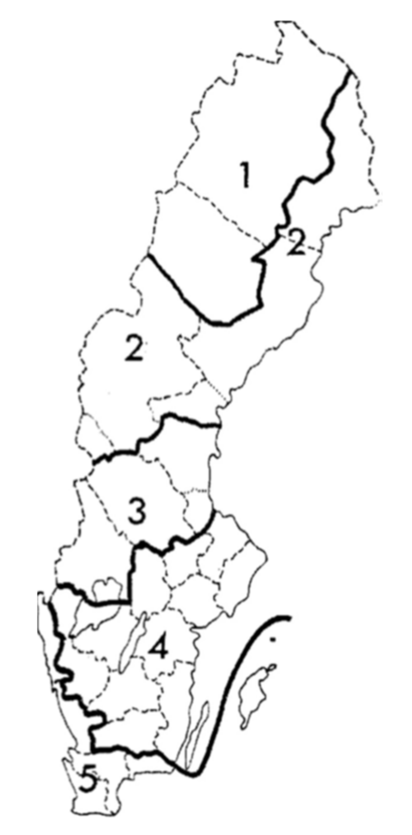
• If such changes are present, to analyse if the direction of change varies among four regions in Sweden, stretching from hemiboreal to northern boreal regions.
• To explore factors that might have contributed to the identified changes.

2. Materials and Methods

2.1. Study Area

The study area comprises all of Sweden except the southernmost part (temperate region) and follows the regional delineation used in the Swedish NFI (Figure 1). About two-thirds of the area is covered by forests (based on the FAO, Food and Agriculture Organization of the United Nations, forest definition; [18]) with a total area of 28 million hectares [15]. Industrial forestry has occurred on most of the area since the early 1800s, with large-scale implementation of clearcut forestry from the middle of the 1900s [19].

2.2. NFI Data

The Swedish NFI includes a network of systematically located sampled plots where many variables, including the cover of species in the ground vegetation, are monitored [17]. The NFI design is based on clusters of sample plots in square-formed tracts (4–8 plots per tract depending on region). The plots are evenly spaced and located around the tract perimeter with the length of tract side varying from 300 to 1200 m among regions. For our analysis, we used data on cover of vascular plants, mosses and lichens in 100 m² permanent (with repeated inventories) circular plots during one full inventory cycle with the first and second inventory year separated by 10 years. The first year of inventory ranged from 1995 to 2003. The cover estimates include surveyor variation, but this variation is considered relatively small compared to random errors [20]. Hence, we base all our analyses on a pair-wise comparison of plots with a 10-year time interval between inventories. We only included plots on productive forestland (annual growth > 1 m³ ha⁻¹ yr⁻¹). As auxiliary information we extracted data on thinnings taking place within 10 years prior to the first inventory (0/1), stand productivity (m³ ha⁻¹ yr⁻¹), change in basal area (m² ha⁻¹) over the 10-year period, change in canopy cover (%) over the 10-year period and stand maturity class at the first inventory (4 classes of old/mature forest;

Table 1. Stand age (basal area weighted average, year) and fraction (%) of total number of sample plots in the different stand maturity classes (according to the Swedish National Forest Inventory (NFI)) included in the study.

	Maturity Class *
Region	33	34	41	42
1	70 (17.5%)	89 (5.9%)	102 (32.0%)	156 (44.6%)
2	64 (20.0%)	89 (8.6%)	96 (25.9%)	139 (45.5%)
3	55 (26.5%)	77 (7.0%)	81 (20.3%)	122 (46.3%)
4	50 (23.1%)	69 (6.8%)	70 (26.1%)	99 (44.1%)

* 33 = thinning stage with mean DBH >20 cm, less than minimum felling age; 34 = thinning stage with mean DBH >20 cm, above minimum felling age; 41 = Final felling stage, but age below recommended for final felling; 42 = Final felling stage above recommended age for final felling.

). The stand maturity classes included in the study have a minimum requirement of dominant and subdominant trees with a diameter at breast height (DBH) larger than 20 cm and are based on stand age in relation to lowest allowed and lowest recommended harvest age.

The Swedish NFI includes inventory of 70 forest-floor species, or combinations of species not identified individually in the field [21]. Several of these species are relatively rare. For a species to be included in our analysis it had to occur in at least 20 sample plots in a region and be present in at least three of four regions. Although fulfilling the inclusion criteria, three species typical for early successional stages were excluded (i.e., Epilobium angustifolium, Rubus ideaus and Geranium sylvaticum), since they are assumed to be in a transient successional phase also in mature forests. With the applied selection criteria, our analysis is based on 25 species and more than 12,500 individual species by region observations across 1300 study plots in each of the two inventory years.

2.3. Statistical Analysis

The change in abundance was analysed by calculating a 95% confidence interval around the mean absolute change in cover between the two inventories for individual species and six major species groups (graminoids, herbs, dwarf shrubs, spore plants, lichens and mosses) within individual regions. For the species group analysis, we included all species surveyed by the NFI. Although the NFI plots are located in clusters (tracts), we assume that observed changes are independent among plots. The distance between plots is several hundreds of meters and even for the most frequent species, on average only two to three plots per tract are included in the analysis. This assumption was also made in several recent studies using vegetation data from the NFI (e.g., [4,6]).

The influence of the four stand variables on the change in abundance was explored by linear regression, using the function “lm” in the statistical software R [22]. The analysis was exploratory since there are a very large number of potential models that can be developed and the purpose was not to predict change per se. Rather, we wanted to exclude factors relating primarily to successional aspects and focus on change that is more likely due to other abiotic factors. Hence, we considered region as a “block” in the analysis, and each of the four stand variables was tested individually for a change in percentage cover for each species (see Appendix A,

Table A1. Effects of stand productivity, basal area change, presence of thinning 10 years prior to first inventory period and stand Maturity class (see Table 1) on the change in cover during the studied 10-year period. Values are p-values from linear models with regions treated as a block in the analysis. Bold numbers indicate a significant effect. N denotes number of plots where the species occurred.

Species	Stand Productivity	Basal Area Change	Thinning Prior First Inventory	Maturity Class	N
Graminoids
Broad leaved grasses	0.044	<0.001	0.066	0.160	482
Narrow leaved grasses	0.613	0.431	0.397	0.204	953
Carex globularis	0.606	0.686	0.014	0.527	240
Herbs
Anemone nemorosa	0.429	0.036	0.538	0.048	195
Maianthemum bifolium	0.111	0.963	0.299	0.067	470
Melampyrum spp.	0.718	0.099	0.010	0.368	762
Oxalis acetosella	0.325	0.844	0.287	0.020	259
Dwarf shrubs
Calluna vulgaris	0.081	0.482	<0.001	0.320	442
Empetrum nigrum	0.698	0.346	0.854	0.866	486
Rubus chamaemorus	0.634	0.291	0.447	0.334	172
Rhododendron tomentosum	0.857	0.570	0.066	0.595	133
Vaccinium myrtillus	0.459	0.318	0.004	0.018	1230
Vaccinium uliginosum	0.374	0.233	0.467	0.434	325
Vaccinium vitis-idae	0.777	0.633	0.300	0.232	1143
Spore plants
Equisetum sylvaticum	0.482	0.258	0.347	0.503	236
Gymnocarpium dryopteris	0.435	0.351	0.828	0.234	222
Lycopodiaceae	0.818	0.552	0.271	0.037	278
Tall ferns	0.096	0.528	0.611	0.474	124
Lichens
Cladonia spp. excl. Cladina	0.151	0.46	0.704	0.570	799
Cladonia grp. Cladina	<0.001	0.608	0.401	<0.001	607
Other ground lichens	0.003	0.623	0.572	0.443	626
Mosses
Hylocomium splendens	0.148	0.083	0.086	0.046	1194
Pleurozium schreberi	0.718	0.070	0.007	0.268	1262
Polytrichum spp.	0.825	0.997	0.186	0.517	465
Sphagnum spp.	0.275	0.513	0.686	0.257	629

). For continuous variables (stand productivity and change in basal area), we only report the degree of explanation (adjusted R²) when the factor significantly influenced percentage cover change. For the categorical factors (thinning prior to first inventory and stand maturity class) we provide for each class the percentage cover change for individual species when these factors were significant.

To explore the responses of individual species we selected a set of Ecological Indicator Values (EIV) [23] that directly link to the main factors influencing the abundance of vascular plants in boreal forests. We compared six EIVs (heat requirement, continentality, light, moisture, soil reaction (pH) and nitrogen) for species showing significant change with the EIVs for the other plant species monitored by the NFI by calculating mean EIVs for each of the groups. If the mean EIV differed by more than one unit, we consider this as an indication that the factor influenced the observed change (see Appendix B,

Table A2. Individual and mean EIV for species showing decreasing cover in this study and mean value for all other species included in the Swedish NFI. No. of regions indicates the number of regions where the species significantly decreased in cover.

Species	No. of Regions	Heat	Continentality	Light	Moisture	Soil (pH)	Nitrogen
Species included with decreasing cover
Maianthemum bifolium	3	4	4	3	4	3	3
Narrow leaved grasses *	3	2	5	4	4	3	5
Melampyrum spp.**	2	3.5	5.5	4.5	3.5	3	3.5
Equisetum sylvaticum	2	3	5	4	5	2	3
Carex globularis	2	4	8	4	6	2	2
Rubus chamaemorus	2	3	5	4	6	1	2
Vaccinium myrtillus	2	3	5	4	5	2	2
Empetrum nigrum	2	3	6	5	6	2	3
Gymnocarpium dryopteris	1	3	5	2	4	4	6
Oxalis acetosella	1	4	4	2	5	4	5
Anemone nemorosa	1	5	4	4	5	4	6
Calluna vulgaris	1	5	5	5	4	2	2
Vaccinium uliginosum	1	2	6	5	6	2	2
Mean value		3.5	5.2	3.8	4.9	2.9	3.4
NFI species (N=36) not included in the study or not showing decreased cover
Mean value		4.8	4.9	4.0	5.4	4.7	5.4

* EIV used for Avenella flexuosa, which is by far the most dominant species in this group. ** Average EIV for M. pratense and M. sylvaticum, which are by far the two most dominant Melampyrum species in the studied forests.

).

An NMDS ordination was performed for the six major species groups to examine the effects of inventory time and region on percentage cover. The functions “metaMDS” and “envfit” in R-package “vegan” [24] were used for the analysis, with a solution converging for a 4-dimensional solution based on a Bray–Curtis dissimilarity matrix (final stress 0.0618). Significance test of inventory time (first or second inventory) and region was based on 1000 permutations. For the full data set of all species, no converging solution was possible to obtain. Further details on ordination analysis are given in Appendix C.

3. Results

3.1. Stand Structure

On average, 17.5% of the 1300 sample plots was thinned during the 10-year period prior to the first inventory, ranging from 9.4% in region 2 to 25.5% in region 4. The basal area increased as expected, with about 10% across the regions (

Table 2. Changes in basal area and canopy cover over the 10-year period.

	First Inventory		Second Inventory
Region	Mean	SD	Mean	SD	N	Difference
Basal area (m2 ha−1)
1	20.1	8.02	22.1	8.33	294	2.0
2	24.8	9.86	27.1	10.48	312	2.2
3	26.30	10.53	29.2	10.99	398	2.9
4	28.0	9.69	30.7	10.75	296	2.8
Total	24.9	10.05	27.4	10.72	1300	2.5
Canopy cover (%)
1	55.6	16.77	60.9	15.21	46	5.2
2	56.1	18.42	57.0	13.38	44	1.0
3	50.9	17.86	63.9	11.73	55	13.0
4	58.5	12.72	63.2	12.19	34	4.7
Total	54.8	16.96	61.3	13.36	179	6.5

). Canopy cover estimates were only available for a limited number of plots (179) and indicate an increase of about 12% across the regions (Table 2).

3.2. Change in Species Abundance

We found significant changes in the abundance of many species in several regions during the 10-year period. Out of 93 analysed species–region combinations, 37 showed a significant decrease in cover, whereas only 4 combinations (all mosses) increased (

Table 3. Species showing significant changes (p < 0.05) in cover in individual regions (see Figure 1). Initial cover denotes the average cover for the first inventory year while the absolute change and the relative change refers to the average change occurring after 10 years. N refers to the number of plots included in the analysis. The 95% confidence interval for the absolute change is defined by its two limits: the Lower Confidence Limit (LCL) and the Upper Confidence Limit (UCL).

			Cover (%)
Species *	Region	N	Initial	Change Absolute (Relative)	LCL	UCL
Graminoids
Broad leaved grasses	3	187	6.8	−1.7 (−25%)	−3.04	−0.36
Broad leaved grasses	4	135	7.6	−2.3 (−30%)	−3.97	−0.53
Carex globularis	2	69	1.7	−0.6 (−34%)	−1.01	−0.11
Carex globularis	3	80	2.0	−0.8 (−42%)	−1.51	−0.19
Narrow leaved grasses	2	240	3.4	−1.2 (−35%)	−1.73	−0.64
Narrow leaved grasses	3	274	5.0	−2.0 (−40%)	−3.08	−0.97
Narrow leaved grasses	4	208	5.8	−2.1 (−36%)	−3.32	−0.92
Herbs
Anemone nemorosa	3	107	2.1	−0.8 (−38%)	−1.55	−0.02
Maianthemum bifolium	1	62	3.7	−1.6 (−43%)	−3.03	−0.21
Maianthemum bifolium	3	160	1.7	−0.4 (−26%)	−0.80	−0.09
Maianthemum bifolium	4	111	1.9	−0.9 (−49%)	−1.42	−0.43
Melampyrum spp.	3	245	1.2	−0.3 (−27%)	−0.62	−0.01
Melampyrum spp.	4	155	1.0	−0.3 (−31%)	−0.52	−0.07
Oxalis acetosella	2	89	3.4	−1.3 (−38%)	−2.17	−0.43
Dwarf shrubs
Calluna vulgaris	3	164	5.3	−0.9 (−16%)	−1.68	−0.05
Empetrum nigrum	3	93	3.7	−1.1 (−29%)	−1.82	−0.31
Empetrum nigrum	4	27	1.2	−0.8 (−68%)	−1.21	−0.42
Rubus chamaemorus	1	52	4.3	−2.1 (−50%)	−3.92	−0.34
Rubus chamaemorus	3	49	4.2	−1.5 (−36%)	−2.85	−0.19
Vaccinium myrtillus	1	291	26.2	−5.8 (−22%)	−7.51	−4.07
Vaccinium myrtillus	2	307	22.6	−4.0 (−17%)	−5.49	−2.42
Vaccinium uliginosum	4	52	5.6	−1.8 (−31%)	−3.43	−0.08
Spore plants
Equisetum sylvaticum	1	80	3.5	−2.2 (−64%)	−3.38	−1.04
Equisetum sylvaticum	2	91	1.4	−0.5 (−35%)	−0.82	−0.14
Gymnocarpium dryopteris	1	52	6.8	−3.0 (−44%)	−5.02	−1.01
Lichens
Cladonia spp. excl. Cladina	2	196	0.4	−0.1 (−32%)	−0.23	−0.03
Cladonia spp. excl. Cladina	4	162	0.4	−0.2 (−48%)	−0.28	−0.07
Cladonia grp. Cladina	2	162	6.3	−3.0 (−47%)	−4.15	−1.78
Cladonia grp. Cladina	3	184	8.3	−2.5 (−30%)	−3.56	−1.47
Cladonia grp. Cladina	4	81	2.8	−0.9 (−33%)	−1.85	−0.02
Other ground lichens	2	151	0.9	−0.2 (−25%)	−0.39	−0.03
Other ground lichens	3	195	1.1	−0.4 (−33%)	−0.68	−0.05
Mosses
Hylocomium splendens	3	358	16.9	3.6 (21%)	1.82	5.34
Hylocomium splendens	4	269	14.3	5.7 (40%)	3.59	7.79
Pleurozium schreberi	1	293	36.2	−5.9 (−16%)	−8.39	−3.40
Pleurozium schreberi	3	383	22.7	2.2 (10%)	0.46	3.94
Pleurozium schreberi	4	276	22.5	−4.4 (−20%)	−6.64	−2.18
Polytrichum spp.	2	127	4.1	−1.2 (−28%)	−2.09	−0.21
Sphagnum spp.	1	120	21.8	−3.6 (−17%)	−6.31	−0.90
Sphagnum spp.	2	157	20.2	−3.0 (−15%)	−5.03	−0.93
Sphagnum spp.	4	149	21.3	3.4 (16%)	0.56	6.30

* In addition, the following species and species groups did not show significant change in any species–region combination; Vaccinium vitis-idea, Rhododendron tomentosum, Lycopodiaceae and tall ferns.

), that is, about 44% of the species–region combinations showed a significant change in cover. Albeit the absolute change was relatively small, the relative change was high. For species that decreased, the average relative decrease was 34%, while those that increased changed on average with 22%. The number of species showing significant change ranged from 7 to 11 decreasing species and from 0 to 2 increasing species per region.

3.3. Factors Correlating with Change in Cover

The explored linear regression models (including stand productivity, presence of thinning during 10 years prior to the first inventory, change in basal area during the 10-year period and stand maturity class) were in most cases nonsignificant (see Appendix A, Table A1). However, some of the independent variables influenced cover of the species:

Stand productivity—Reindeer lichens (Cladonia grp. Cladina) and other ground lichens tended to decrease their cover less on plots with higher forest productivity, while broad-leaved grasses decreased more at high productivity plots. However, the models were very weak and explained 1% or less of the change in cover.

Change in basal area—Anemone nemorosa and broad-leaved grasses decreased more at sites with a higher increase in basal area. However, these models only explained about 2% of the change in cover.

Thinning before the first period—Melampyrum spp., Vaccinium myrtillus and Calluna vulgaris decreased in unthinned plot and increased in thinned plots. By contrast, Carex globularis and Pleurozium schreberi were negatively influenced by thinning (

Table 4. Relative cover change for species where thinning occurred during 10 years prior to first inventory significantly (p < 0.05) explained the observed variation. Sample size in parenthesis.

	Relative cover Change (%) in Un-Thinned and Thinned Stands
Species	Unthinned	Thinned
Melampyrum spp.	−33% (635)	8% (127)
Vaccinium myrtillus	−15% (1033)	6% (197)
Calluna vulgaris	−20% (358)	59% (84)
Carex globularis	−32% (217)	−69% (23)
Pleurozium schreberi	−5% (1052)	−16% (210)

).

Stand maturity class—The change in cover of some species (Oxalis acetosella, Anemone nemorosa, Vaccinium myrtillus, and Cladonia grp. Cladina) maintained their cover better in the younger maturity classes, except for Cladonia grp. Cladina, which decreased most in the youngest class. Lycopodiaceae showed varying cover change in the different maturity classes (

Table 5. Relative change in cover of species where maturity class (stand age proxy) was a significant (p < 0.05) factor explaining the observed variation. The sample size in given in parenthesis. For definition of maturity classes see Table 1.

	Relative Cover Change (%) in Maturity Classes
Species	33	34	41	42
Oxalis acetosella	10% (40)	−59% (14)	−46% (72)	−21% (133)
Anemone nemorosa	8% (51)	−36% (16)	−25% (49)	−65% (79)
Vaccinium myrtillus	−1% (185)	−13% (71)	−14% (314)	−14% (660)
Lycopodiaceae	−39% (41)	74% (15)	−2% (70)	−28% (153)
Hylocomium splendens	34% (190)	23% (73)	9% (296)	9% (635)
Cladonia grp. Cladina	−54% (77)	−29% (38)	−28% (165)	−22% (327)

).

The mean value of three EIVs for the vascular plants showing decreasing cover, differed with more than one unit compared to the other species monitored in the NFI plots (Appendix B, Table A2); Heat EIV was 1.3 units lower, Soil pH EIV was 1.8 units lower and Nitrogen EIV was 2 units lower. Hence, the decreasing species occurred in colder climates and less productive forests compared to the other forest species.

3.4. Change in Species Groups

When combining the species into six functional groups, most of the groups showed a significant decrease in their cover. Only mosses in region 3 increased (relative increase of 9%). The change was not significant for seven of the 24 species group–region combinations (

Table 6. Change in cover of six species groups in four regions (see Figure 1). Initial cover denotes the average cover for the first inventory year, while the absolute change and the relative change refer to the average change occurring after 10 years. N refers to the number of plots included in the analysis. The 95% confidence interval for the absolute change is defined by its two limits: the Lower Confidence Limit (LCL) and the Upper Confidence Limit (UCL). NS denotes nonsignificant (p > 0.05) change.

		Cover (%)
Species Group	N	Initial	Change Absolute (Relative)	LCL	UCL	Direction
Graminoids
Region 1	245	3.6	−0.5 (−13%)	−0.99	0.06	NS
Region 2	254	6.0	−1.3 (−22%)	−2.15	−0.54	Decrease
Region 3	332	10.2	−2.8 (−27%)	−4.16	−1.43	Decrease
Region 4	250	10.7	−2.6 (−24%)	−4.12	−1.09	Decrease
Herbs
Region 1	179	3.0	−1.0 (−33%)	−1.57	−0.37	Decrease
Region 2	230	4.6	−0.9 (−19%)	−1.51	−0.19	Decrease
Region 3	309	3.8	−0.8 (−20%)	−1.34	−0.17	Decrease
Region 4	225	4.1	−1.1 (−28%)	−1.93	−0.32	Decrease
Dwarf shrubs
Region 1	269	56.4	−8.0 (−14%)	−10.49	−5.56	Decrease
Region 2	286	49.7	−6.7 (−14%)	−8.91	−4.57	Decrease
Region 3	354	33.7	−1.7 (−5%)	−3.55	0.17	NS
Region 4	277	24. 8	−0.8 (−3%)	−2.70	1.12	NS
Spore plants *
Region 1	159	5.0	−2.2 (−44%)	−3.23	−1.11	Decrease
Region 2	175	5.1	−1.3 (−25%)	−2.19	−0.36	Decrease
Region 3	124	2.9	−0.3 (−9%)	−0.95	0.44	NS
Region 4	80	2.5	0.4 (15%)	−0.40	1.18	NS
Lichens
Region 1	221	5.7	−0.6 (−11%)	−1.68	0.48	NS
Region 2	241	7.3	−3.0 (−42%)	−4.08	−1.99	Decrease
Region 3	308	6.9	−2.0 (−28%)	−2.79	−1.12	Decrease
Region 4	222	1.6	−0.4 (−26%)	−0.85	−0.01	Decrease
Mosses
Region 1	269	79.4	−7.6 (−10%)	−10.29	−4.95	Decrease
Region 2	290	79.1	−3.2 (−4%)	−5.91	−0.42	Decrease
Region 3	367	63.6	5.9 (9%)	3.56	8.33	Increase
Region 4	280	57.4	2.2 (4%)	−0.78	5.09	NS

* Including ferns, Equisetum spp. and Lycopodiaceae.

). The average relative cover change for decreasing species groups was 23%, ranging from 4% to 44%. Herbs significantly decreased in all regions, while graminoids and lichens decreased in three regions.

The NMDS ordination of the six groups mirrors the general pattern of significant change in most species groups (Figure 2). The ordination highlights that the composition differs among regions and that it is change over time (both factors significant, p < 0.01). However, only a minor fraction of the total variation in species composition was explained. The ordination suggests that the composition becomes more similar and moves towards the composition in region 1, with a stronger relative dominance of mosses and dwarf shrubs. Additional details on the ordination results are presented in Appendix C.

4. Discussion

Our analysis of the change in cover of ground vegetation in mature boreal forests shows a rapid and significant decrease for many of the studied species and most species groups. We recognize that our data do not allow for a formal cause-and-effect analysis of the reasons behind these changes, but the results highlight the need to explore potential factors that contribute to our observations. Our data are large and for most species and species groups include several hundreds of randomly distributed plots throughout boreal and hemiboreal Sweden, adding strong statistical support for the observed patterns.

Previous studies using NFI data from Sweden and Finland have demonstrated clear effects of forest management on forest-floor vegetation [4,6,25,26]. Their results can mostly be attributed to the direct effects of forest management (clearcut harvesting and thinning) and the subsequent succession in forest-floor vegetation. Changes in light, nutrient and moisture availability are obvious after forestry interventions, and vegetation dynamics reflect these changes in abiotic conditions. Two recent studies [25,26] acknowledged that climate change may also play a role in observed changes, but the impact is likely minor compared to the effects of the conducted forest management operations. In our case, we have as far as possible removed the direct effects of management activities by focusing on mature forest stands that have not been subjected to major anthropogenic disturbances.

4.1. Succession

Although the study plots have not been recently subject to major management interventions, successional transitions may still potentially explain at least part of the observed changes. Several studies from Fennoscandia have described the pattern of vegetation dynamics after disturbance by using comparable data. For example, in a study from northern Finland [27], succession after disturbance was studied in both managed (after clearcutting) and natural forests (after forest fire), ranging from recently disturbed sites to overmature stands (>100 years). In the managed forest stands, Vaccinium myrtillus increased in cover from mature to overmature forests. Also in Swedish forests, the cover of V. myrtillus increased up to a forest age of about 120 years [28]. This was not the case in our study. Here the cover of V. myrtillus decreased in the two northern regions and remained rather stable in the two southern regions. Hence, our results are more in line with recent studies in Sweden [5,6] showing a general decrease of V. myrtillus and other dwarf shrubs, which could be attributed to increasing stand density across Swedish forests (see [15]). These contrasting observations add to a somewhat puzzling variation in the abundance of this keystone species in Fennoscandian forests [4]. Probably there is an interaction between stand density and stand age in these studies. The importance of stand density is supported by our data, since V. myrtillus decreased less in stands thinned prior to the first inventory period and in younger stand maturity-classes.

It is well-established that light availability, and hence canopy cover, in combination with precipitation strongly affect lichen growth [29,30]. In a study comparing lichen growth rate across sites with different canopy cover, it was shown that canopy cover over 60% reduced growth of two common terricolous lichens (Cladonia stellaris and Cetraria islandica) [31]. This suggests that increasing canopy cover could result in decreased abundance of ground lichens also in our data set. During the studied 10-year period, the canopy cover increased with on average about 6%, from just below to just above the 60% threshold. It should also be noted that the basal area in mature forests in our dataset is higher than in the cited study [31].

However, if our observed changes would be mainly associated with a successional trajectory from younger to older forest, with increasing basal area and canopy cover, we would expect to see consistent effects of the changes in basal area during the study period as well effects of thinning events prior to the 10-year inventory period. Our analyses clearly indicate that this is not the case. We found only minor effects of the change in basal for a few species, that is, for Anemone nemorosa, broad-leaved grasses and for three species that increased in thinned stands and decreased in unthinned stands (Table 4). This suggests that the observed changes in cover of major plant groups are not only driven by successional change and that other factors may contribute to the changes in vegetation.

4.2. Climate

A significant increase in average temperature and precipitation was observed throughout Sweden from the early 1990s. Compared to the reference period 1961–1990, the average temperature in Sweden was 1.0 degrees higher during the inventory period 1995–2014, with a 9% increase in precipitation [32]. The long-term trend with a warmer climate is clear, and the response of the vegetation may well be associated with this trend. Given that our observed changes cannot be fully explained by succession, climate change should at least be considered a contributing factor. This is supported by the EIV analysis, since the decreasing species tended to be more associated with colder environments than the other vascular plants monitored by the NFI.

A warmer climate extends the vegetation period and may shift the competitive balance among species, with some winners and some losers. It is well-established that soil warming has significant effects on ground vegetation in tundra habitats [33]. However, it is likely that closed canopy forests mediate the effects of soil temperature on ground vegetation [34]. In a long-term experimental study of soil warming, Hedwall et al. [35] found a strong initial vegetation response in young forests, but the long-term effects were less clear, except that moss cover increased as the forest became older. The soil temperature during winter is strongly connected to the insulating effect of snow cover [36]. Milder winters in the south will give a less consistent snow cover, which may increase soil temperature. Hence, we hypothesize that increased temperature may contribute to the observed increase in moss cover in southern Sweden. By contrast, a decrease in snow cover in northern regions may result in stronger ground frost. This has been shown to have dramatic effects on ground vegetation, with significant decrease in the cover of understory vegetation and mosses [37], in accordance with our observations.

An increase in precipitation should favour species and species groups typical of more moist conditions. However, our results contradict this since plants typical for moist forests (Equisetum sylvaticum, Rubus chamaemorus, Carex globularis and Sphagnum spp.) also decreased in cover. Neither do the EIVs provide any indication that species associated with moist habitats were favoured.

4.3. Nitrogen Deposition

Deposition of atmospheric nitrogen is a factor known to have significant impact on boreal forest ground vegetation [38]. There is a clear gradient through Sweden with higher deposition in the southwest and lower towards the north [39,40]. Nitrogen deposition has decreased since the 1980s across Europe [41]. However, the change is not as evident in Sweden, besides an indicative trend of decreasing nitrogen deposition in the southwestern part (i.e., including parts of region 4) since around year 2000, and for long time series in northern regions [40]. Yet, the EIV analysis suggests that species associated with more nutrient-poor environments (low soil pH and less nitrogen demanding) are overrepresented among species showing decreasing cover.

In experimental studies it has been shown that narrow-leaved grasses (dominated by Deschampsia flexuosa) and herbs increase with increasing nitrogen deposition while dwarf shrubs and lichens decrease [14,42]. In comparison with our results, the effect of nitrogen corresponds to the decline in dwarf shrubs and lichens, but not for narrow-leaved grasses and herbs, since all these species groups decline in mature Swedish forests. It should be noted, however, that even if experimental studies often show clear effects on ground vegetation, the effect of the overall atmospheric deposition of nitrogen is less evident, mainly because experimental doses applied are commonly much higher than background deposition [38]. This complicates the interpretation of our results.

4.4. Time Lags in Responses

Most of the studied species and species groups are clonal and long-lived. Hence, although abiotic conditions change, associated changes in cover and occurrence of plants likely include time lags, that is, integrating effects over a longer time period than the studied 10-year period. For instance, major distributional and abundance changes in Finnish ground vegetation are predicted up to mid-late 21st century due to increased temperature [9], and hence highlight trends over longer time periods. When evaluating potential factors behind the observed changes, this implies that increasing stand age and changes in climate and nitrogen deposition occur in parallel time scales, which might require several decades before fully manifested.

4.5. Conclusions

We have shown large changes in the ground vegetation in mature Swedish forests over a relatively short time period (10 years). These changes may imply ecosystem-level impacts on the function of boreal forests [43]. At this stage, we cannot attribute the observed changes to a single factor. The changes likely result from a combination of succession, climate change and nitrogen deposition, and where time lags complicate the interpretation. This confirms the conclusion from the review by [16] that it is necessary to consider both previous land management and functional properties of plant communities when analysing and modelling effects of the ongoing global change.

References

1. Nilsson, M.-C.; Wardle, D.A. Understory vegetation as a forest ecosystem driver: Evidence from the northern Swedish boreal forest. Front. Ecol. Environ. 2005, 3, 421–428. [Google Scholar] [CrossRef]
2. Hart, S.A.; Chen, H.Y.H. Understory Vegetation Dynamics of North American boreal forests. Crit. Rev. Plant Sci. 2006, 25, 381–397. [Google Scholar] [CrossRef]
3. Bergeron, Y. Species and stand dynamics in the mixed woods of Quebec’s southern boreal forest. Ecology 2000, 81, 1500–1516. [Google Scholar] [CrossRef]
4. Bergstedt, J.; Milberg, P. The impact of logging intensity on field-later vegetation in Swedish boreal forests. For. Ecol. Manag. 2001, 154, 105–115. [Google Scholar] [CrossRef]
5. Hedwall, P.O.; Brunet, J.; Nordin, A.; Bergh, J. Changes in the abundance of keystone forest floor species in response to changes of forest structure. J. Veg. Sci. 2013, 24, 296–306. [Google Scholar] [CrossRef]
6. Hedwall, P.O.; Gustafsson, L.; Brunet, J.; Lindbladh, M.; Axelsson, A.-L.; Strengbom, J. Half a century of multiple anthropogenic stressors has altered northern forest understory plant communities. Ecol. Appl. 2019, 29, e01874. [Google Scholar] [CrossRef]
7. Bobbink, R.; Hicks, K.; Galloway, J.; Spranger, T.; Alkemade, R.; Ashmore, M.; Bustamante, M.; Cinderby, S.; Davidson, E.; Dentener, F.; et al. Global assessment of nitrogen deposition effects on terrestrial plant diversity: A synthesis. Ecol. Appl. 2010, 20, 30–59. [Google Scholar] [CrossRef] [PubMed] [Green Version]
8. Phoenix, G.K.; Emmett, B.A.; Britton, A.J.; Caporn, S.J.M.; Dise, N.B.; Helliwell, R.; Jones, L.; Leake, J.R.; Leith, I.D.; Sheppard, L.J.; et al. Impacts of atmospheric nitrogen deposition: Responses of multiple plant and soil parameters across contrasting ecosystems in long-term field experiments. Glob. Chang. Biol. 2012, 18, 1197–1215. [Google Scholar] [CrossRef]
9. Villén-Perez, S.; Heikkinen, J.; Salemaa, M.; Mäkipää, R. Global warming will affect the maximum potential abundance of boreal plant species. Ecography 2020, 43, 801–811. [Google Scholar] [CrossRef] [Green Version]
10. Forest Europe 2015. In Proceedings of the State of Europe’s Forests 2015, Ministerial Conference on the Protection of Forests in Europe, Madrid, Spain, 20–21 October 2015.
11. Wulder, M.A.; Campbell, C.; White, J.C.; Flannigan, M.; Campbell, I.D. National circumstances in the international circumboreal community. For. Chron. 2007, 83, 539–556. [Google Scholar] [CrossRef] [Green Version]
12. IPCC. Climate Change 2014: Summary for Policymakers, Synthesis Report. Contribution of Working Groups I, II and III to the Fifth Assessment Report of the Intergovernmental Panel on Climate Change; IPCC, Pachauri, R.K., Meyer, L.A., Eds.; IPCC: Geneva, Switzerland, 2014; p. 151. [Google Scholar]
13. Tamm, C.O. Nitrogen in terrestrial ecosystems. Questions of productivity, vegetational change and ecosystem stability. Ecol. Stud. 1991, 81, 1–116. [Google Scholar]
14. Strengbom, J.; Nordin, A. Commercial forest fertilization causes long-term residual effects in ground vegetation of boreal forests. For. Ecol. Manag. 2008, 256, 2175–2181. [Google Scholar] [CrossRef]
15. SLU 2019. Forest statistics 2019–Official Statistics of Sweden; Swedish University of Agricultural Sciences: Umeå, Sweden, 2019. [Google Scholar]
16. Perring, M.P.; Bernhardt-Römermann, M.; Baeten, L.; Midolo, G.; Blondeel, H.; Depauw, L.; Landuyt, D.; Maes, S.L.; De Lombaerde, E.; Carón, M.M.; et al. Global environmental change effects on plant community composition trajectories depend upon management legacies. Glob. Chang. Biol. 2018, 24, 1722–1740. [Google Scholar] [CrossRef] [PubMed] [Green Version]
17. Fridman, J.; Holm, S.; Nilsson, M.; Nilsson, P.; Ringvall, A.H.; Ståhl, G. Adapting National Forest Inventories to changing requirements–the case of the Swedish National Forest Inventory at the turn of the 20th century. Silva Fenn. 2014, 48, 1095. [Google Scholar] [CrossRef] [Green Version]
18. FAO. Global Forest Resources Assessment. Terms and Definitions; Food and Agriculture Organization of the United Nations (FAO), Forestry Department: Rome, Italy, 2010. [Google Scholar]
19. Östlund, L.; Zackrisson, O.; Axelsson, A.-L. The history and transformation of a Scandinavian boreal forest landscape since the 19th century. Can. J. For. Res. 1997, 27, 1198–1206. [Google Scholar] [CrossRef]
20. Milberg, P.; Bergstedt, J.; Fridman, J.; Odell, G.; Westerberg, L. Observer bias and random variation in vegetation monitoring data. J. Veg. Sci. 2008, 19, 633–644. [Google Scholar] [CrossRef] [Green Version]
21. Odell, G. (Ed.) Fältinstruktion 2018: Riksinventering av Skog; Swedish University of Agricultural Sciences: Umeå, Swedish, 2018. [Google Scholar]
22. R Core Team. R: A Language and Environment for Statistical Computing; R Foundation for Statistical Computing: Vienna, Austria, 2017; Available online: https://www.R-project.org/ (accessed on 20 December 2018).
23. Tyler, T.; Herbertsson, L.; Olofsson, J.; Olsson, P.A. Ecological indicator and traits values for Swedish vascular plants. Ecol. Indic. 2021, 120, 106923. [Google Scholar] [CrossRef]
24. Oksanen, J.; Blanchet, F.G.; Friendly, M.; Kindt, R.; Legendre, P.; McGlinn, D.; Minchin, P.R.; O’Hara, R.B.; Simpson, G.L.; Solymos, M.; et al. Vegan, Community Ecology Package, Version 2.5-2; Available online: http://www.R-project.org/ (accessed on 20 December 2018).
25. Hedwall, P.O.; Brunet, J. Trait variations of ground flora species disentangle the effects of global change and altered land-use in Swedish forests during 20 years. Glob. Chang. Biol. 2016, 22, 4038–4047. [Google Scholar] [CrossRef]
26. Tonteri, T.; Salemaa, M.; Rautio, P.; Hallikainen, V.; Korpela, L.; Merilä, P. Forest management regulates temporal change in the cover of boreal plant species. For. Ecol. Manag. 2016, 381, 115–124. [Google Scholar] [CrossRef]
27. Uotila, A.; Kouki, J. Understorey vegetation in spruce-dominated forests in eastern Finland and Russian Karelia: Successional patterns after anthropogenic and natural disturbances. For. Ecol. Manag. 2005, 215, 113–137. [Google Scholar] [CrossRef]
28. Kardell, L. Occurrence and production of bilberry, lingonberry and raspberry in Sweden’s forests. For. Ecol. Manag. 1980, 2, 285–298. [Google Scholar] [CrossRef]
29. Palmqvist, K. Carbon economy in lichens. New Phytol. 2000, 148, 11–36. [Google Scholar] [CrossRef]
30. Gauslaa, Y.; Palmqvist, K.; Solhaug, K.A.; Holien, H.; Hilmo, O.; Nybakken, L.; Myhre, L.C.; Ohlson, M. Growth of epiphytic old forest lichens across climatic and successional gradients. Can. J. For. Res. 2007, 37, 1832–1845. [Google Scholar] [CrossRef]
31. Cabrajic, A.V.J.; Moen, J.; Palmqvist, K. Predicting growth of mat-forming lichens on a landscape scale–Comparing models with different complexities. Ecography 2010, 33, 949–960. [Google Scholar] [CrossRef]
32. SMHI 2018. Official Data from the Swedish Meteorological and Hydrological Institute. Available online: https://www.smhi.se/klimat/ (accessed on 15 January 2019).
33. Walker, M.D.; Wahren, C.H.; Hollister, R.D.; Henry, G.H.R.; Ahlquist, L.E.; Alatalo, J.M.; Bret-Harte, M.S.; Calef, M.P.; Callaghan, T.V.; Carroll, A.M.; et al. Plant community responses to experimental warming across the tundra biome. Proc. Natl. Acad. Sci. USA 2006, 103, 1342–1346. [Google Scholar] [CrossRef] [Green Version]
34. De Frenne, P.; Rodrıguez-Sanchez, F.; Coomes, D.A.; Baeten, L.; Verstraeten, G.; Vellend, M.; Bernhardt-Römermann, M.; Brown, C.D.; Brunet, J.; Cornelis, J.; et al. Microclimate moderates plant responses to macroclimate warming. Proc. Natl. Acad. Sci. USA 2013, 110, 18561–18565. [Google Scholar] [CrossRef] [PubMed] [Green Version]
35. Hedwall, P.O.; Skoglund, J.; Linder, S. Interactions with successional stage and nutrient status determines the life-form-specific effects of increased soil temperature on boreal forest floor vegetation. Ecol. Evol. 2015, 5, 948–960. [Google Scholar] [CrossRef]
36. Jungqvist, G.; Oni, S.K.; Teutschbein, C.; Futter, M.N. Effect on soil temperature in Swedish boreal forests. PLoS ONE 2014, 9, e93957. [Google Scholar] [CrossRef] [Green Version]
37. Kreyling, J.; Haei, M.; Laudon, H. Absence of snow cover reduces understory plant cover and alters plant community composition in boreal forest. Oecologia 2012, 168, 577–587. [Google Scholar] [CrossRef] [PubMed]
38. Binkley, D.; Högberg, P. Tamm Review: Revisiting the influence of nitrogen deposition on Swedish forests. For. Ecol. Manag. 2016, 368, 222–239. [Google Scholar] [CrossRef]
39. Strengbom, J.; Walheim, M.; Näsholm, T.; Ericson, L. Regional Differences in the Occurrence of Understorey Species Reflect Nitrogen Deposition in Swedish Forests. Ambio 2003, 32, 91–97. [Google Scholar] [CrossRef] [PubMed]
40. Pihl Karlsson, G.; Hellsten, S.; Karlsson, P.E.; Akselsson, C.; Ferm, M. Kvävedepositionen till Sverige: Jämförelse av Depositionsdata Från Krondroppsnätet, Luft- och Nederbördskemiska Nätet Samt EMEP; IVL Swedish Environmental Research Institute Rapport B2030: Stockholm, Sweden, 2012. [Google Scholar]
41. Engardt, M.; Simpson, D.; Schwikowski, M.; Granat, L. Deposition of sulphur and nitrogen in Europe 1900–2050. Model calculations and comparison to historical observations. Tellus B Chem. Phys. Meteorol. 2017, 69, 1328945. [Google Scholar] [CrossRef] [Green Version]
42. Kellner, O.; Redbo-Torstensson, P. Effects of elevated nitrogen deposition on the field-layer vegetation in coniferous forests. Ecol. Bull. 1995, 44, 227–237. [Google Scholar]
43. Wardle, D.A.; Jonsson, M.; Bansal, S.; Bardgett, R.D.; Gundale, M.J.; Metcalfe, D.B. Linking vegetation change, carbon sequestration and biodiversity: Insights from island ecosystems in a long-term natural experiment. J. Ecol. 2012, 100, 16–30. [Google Scholar] [CrossRef] [Green Version]
44. Karlsson, T. Förteckning över svenska kärlväxter. Sven. Bot. Tidskr. 1997, 91, 241–560. [Google Scholar]
45. Stenroos, S.; Velmala, S.; Pykälä, J.; Ahti, T. Lichens of Finland; Botanical Museum, Finnish Museum of Natural History LUOMUS, University of Helsinki: Helsinki, Finland, 2016. [Google Scholar]
46. Hallingbäck, T.; Hedenäs, L.; Weibull, H. Ny checklista för Sveriges mossor. Sven. Bot. Tidskr. 2006, 100, 96–148. [Google Scholar]
Figure 1. Regional delineation of Sweden in the National Forest Inventory. Regions 1–3 span the southern boreal to northern boreal zone; region 4 belongs to the hemiboreal zone. Region 5 (temperate zone) is not included in the present study.
Forests 12 00475 g001
Figure 2. NMDS ordination (dimensions 1 and 2) of six species groups, where filled circles denote average “site scores” for the four regions at the two inventories. Arrows denote the direction of change. Note that, to increase the readability of the figure, the positions of the species group scores do not represent their actual scores along the axes, since these are outside the current axis’s ranges. However, their relative position indicates where they occur in the ordination.
Forests 12 00475 g002