Article

Can a Remote Sensing Approach with Hyperspectral Data Provide Early Detection and Mapping of Spatial Patterns of Black Bear Bark Stripping in Coast Redwoods?

by
Shayne Magstadt
1,
David Gwenzi
1,* and
Buddhika Madurapperuma
1,2
1
Department of Environnemental Science and Management, Humboldt State University, Arcata, CA 95521, USA
2
Department of Forestry and Wildland Resources, Humboldt State University, Arcata, CA 95521, USA
*
Author to whom correspondence should be addressed.
Forests 2021, 12(3), 378; https://doi.org/10.3390/f12030378
Submission received: 22 February 2021 / Revised: 17 March 2021 / Accepted: 18 March 2021 / Published: 22 March 2021
(This article belongs to the Section Forest Inventory, Modeling and Remote Sensing)

Abstract

:
The prevalence of black bear (Ursus americanus) bark stripping in commercial redwood (Sequoia sempervirens (D. Don) Endl.) timber stands has been increasing in recent years. This stripping is a threat to commercial timber production because of the deleterious effects on redwood tree fitness. This study sought to unveil a remote sensing method to detect these damaged trees early and map their spatial patterns. By developing a timely monitoring method, forest timber companies can manipulate their timber harvesting routines to adapt to the consequences of the problem. We explored the utility of high spatial resolution UAV-collected hyperspectral imagery as a means for early detection of individual trees stripped by black bears. A hyperspectral sensor was used to capture ultra-high spatial and spectral information pertaining to redwood trees with no damage, those that have been recently attacked by bears, and those with old bear damage. This spectral information was assessed using the Jeffries-Matusita (JM) distance to determine regions along the electromagnetic spectrum that are useful for discerning these three-health classes. While we were able to distinguish healthy trees from trees with old damage, we were unable to distinguish healthy trees from recently damaged trees due to the inherent characteristics of redwood tree growth and the subtle spectral changes within individual tree crowns for the time period assessed. The results, however, showed that with further assessment, a time window may be identified that informs damage before trees completely lose value.

1. Introduction

Coastal redwoods (Sequoia sempervirens) are a fundamental cultural and economic symbol in Humboldt County, CA and both conservation groups and timber resource companies have put forth efforts to protect this unique and important ecosystem. Redwood trees are one the largest coniferous tree species in the world and is one of four tree species that can grow to exceed 90 m [1]. Redwood trees are known for their fast growth rates and ability to stump sprout, giving them a reproductive advantage [1]. This species is found only along the Pacific Coast of Northern America providing unique habitat for a variety of species [1,2]. For instance, they are nesting sites for the Northern Spotted Owl (Strix occidentalis caurina), listed in 1990 as a threatened species under the Federal Endangered Species Act [3]. Redwood trees often experience disturbances such as fire, landslides, flooding and are also susceptible to pest damage such as fungal invasion [4], and herbivory such as bear bark stripping [5]. The black bear (Ursus amercanus) has been stripping the bark of redwoods for a long time, with official reports published as early as 1955 [6,7,8]. This disturbance threatens commercial timber production by decreasing tree health, increasing disease and pest susceptibility, decreasing growth rate, increasing the mortality rate and ultimately leading to financial loss [6]. In Humboldt County, 15% of annual allowable timber harvest loss in the Hoopa Valley Indian Reservation is due to bear damage resulting in one to two million dollars annual loss [9]. Spatial patterns of black bear bark stripping are difficult to assess, but this behavior tends to occur in the spring and early summer months [6]. Bears will use their claws to remove the outer bark. Once the outer bark layer is removed, bears will use their incisors to scrape and remove the cambium layer, feeding on the nutritious sapwood [10]. Black bears attack the most vigorous pre-rotation age trees, between 10 and 30 years, with a diameter at breast height of 25–50 cm [11]. Bear bark stripping also more frequently occurs after stand improvements, such as thinning, thus defeating the purpose of silvicultural practices [6]. The damage is a result of bears searching for food, and single trees or clusters of trees may be selected often following geographic boundaries like roads, trails, or elevation gradients [7]. This forest disturbance is difficult to assess from ground surveys and satellite imagery alone due to both the spatial scale of redwood forests and the isolated and random nature of bear bark stripping [8].
Examining the economic impact of black bear bark stripping is cumbersome and often unreliable [11]. Cost estimates of bark peeling are difficult to assess due to the uneven spatial distribution of bear populations in the area [9]. Conventionally, aerial surveys are conducted to identify trees or groups of trees with visible canopy discoloration [12]. Observers in fixed wing aircraft manually digitized areas with red or gray crowns but are unable to detect trees in the early attack stage and often misclassify bark stripping with disease and other drivers also causing crown discoloration [11]. Presently, studies quantifying estimates of timber loss associated with bark stripping are limited. Aerial surveys in manned fixed wing aircraft were conducted over 25,900 ha of Douglas-fir forest in Oregon and concluded black bear tree bark foraging resulted in an overall economic loss of $15.1 M or $585 per hectare [13]. Another study compared aerial surveys over 3024 ha of Oregon Douglas-fir timberlands with ground truth data to develop models of the economic cost of damage and was perceived to be around $56 per hectare [12]. Human limitations make detecting tree crowns with recent bark peeling difficult. Therefore, developing new methods to identify early stress will not only eliminate human error but lead to more precise tree health predictions.
Images collected using remote sensing can provide information about the landscape beyond what the human eye can ascertain from aircrafts. The availability of many narrow bands (6 nm FWHM) within hyperspectral data, enables the capturing of unique spectral signatures of healthy and stressed vegetation [14]. The main challenge of early detection of damage is that the changes in the foliage of recently stripped trees is subtle, thus making the detection difficult, especially using the multispectral images. The subtle foliar chemistry changes in the recent bark stripping phase is often manifested in specific narrow bands of the electromagnetic spectrum, which are only observable in hyperspectral sensors [15,16,17,18]. The primary benefit of hyperspectral imaging is, therefore, the large number of narrow acquisition bands, providing more detailed spectral signatures. A spectral signature is simply a measure of reflectance as a function of the reflected wavelength [19]. More specifically, hyperspectral sensors capture a dense, nearly continuous, spectral reflectance signature, collecting a much more detailed data cube capable of discerning health variations caused by environmental stressors, such as bear bark stripping [18]. The narrow band widths are also useful for the derivation of vegetation indices (VI) and band ratios (BR) is being correlated to stress levels, which was a proxy for recent tree attack. The key assumption here being that spectral anomalies related to plant phenology will affect all trees equally unless there are other localized stress inducers affecting tree health (i.e., insect or fungal intrusion). Examples of VIs/BRs developed for early detection of vegetation stress from insect attack, include the Vogelmann “red edge” index or VREI 1 [20]; Red-edge Normalized Difference Vegetation Index (RENDVI) [21,22]; Modified Chlorophyll Absorption Ratio Index (MCARI) [23,24]; Plant Senescing Reflectance Index (PSRI) [25] and empirically derived Normalized Channel Ratios (e.g., Ra − Rb/Ra + Rb, where a and b are specific bands selected on the basis of class separability analysis) [26]. The key concept behind all these indices is the spectral signatures of healthy and damaged trees are significantly, and non-systematically different in enough narrow bands along the spectrum, to enable classification. Aside from the benefits of increased spatial and temporal resolution, unmanned aerial vehicles (UAVs) have been used to integrate higher spectral resolution sensors [18]. To obtain high resolution data, UAVs have emerged as a new and promising method for landscape level surveys [27]. UAV data acquisition and analysis are in their infancy and therefore possess several knowledge gaps in need of more exploration.
Research has attempted tree health detection from tree crowns using the remote sensing techniques. Hyperspectral data is useful for delineation of tree crowns with mean shift segmentation algorithm [28], pixel majority approach [29], watershed segmentation [30], forest discrimination index [31] and automatic object-based crown detection algorithms [32]. There are, however, some limitations with these techniques when delineating individual tree crowns resulting from, for example, overlapping crowns [30], defoliation and discoloration [33], variability of crown morphology, and leaf off and leaf on conditions. Tree health of isolated crowns can be detected using vegetation and disease indices [34], visual tree assessment [33] and reflecting scores [32].
The main objective in this study was to determine which spectral features would be able to recognize and classify redwood trees that have been recently damaged by black bears to facilitate control measures. In particular, this research has focused on the possibility of combining high spectral resolution image sensors with the targeted approach of UAV data acquisition. With this combination of survey tools, land managers can more easily utilize remote sensing to quickly analyze the health and condition of natural resources. A method of early detection of bark stripped trees is crucial for sound forest management as it helps forest managers to anticipate a response to tree mortality by, for example; (a) salvaging timber while it is still valuable, (b) targeting affected trees during thinning operations, or (c) modifying forestry functional unit allocations to address the threatened ecosystem services of interest. More specifically, forestry functional unit allocations can be modified by deciding not to harvest commonly stripped areas and concentrate timber production in areas less vulnerable to bear attack.

2. Materials and Methods
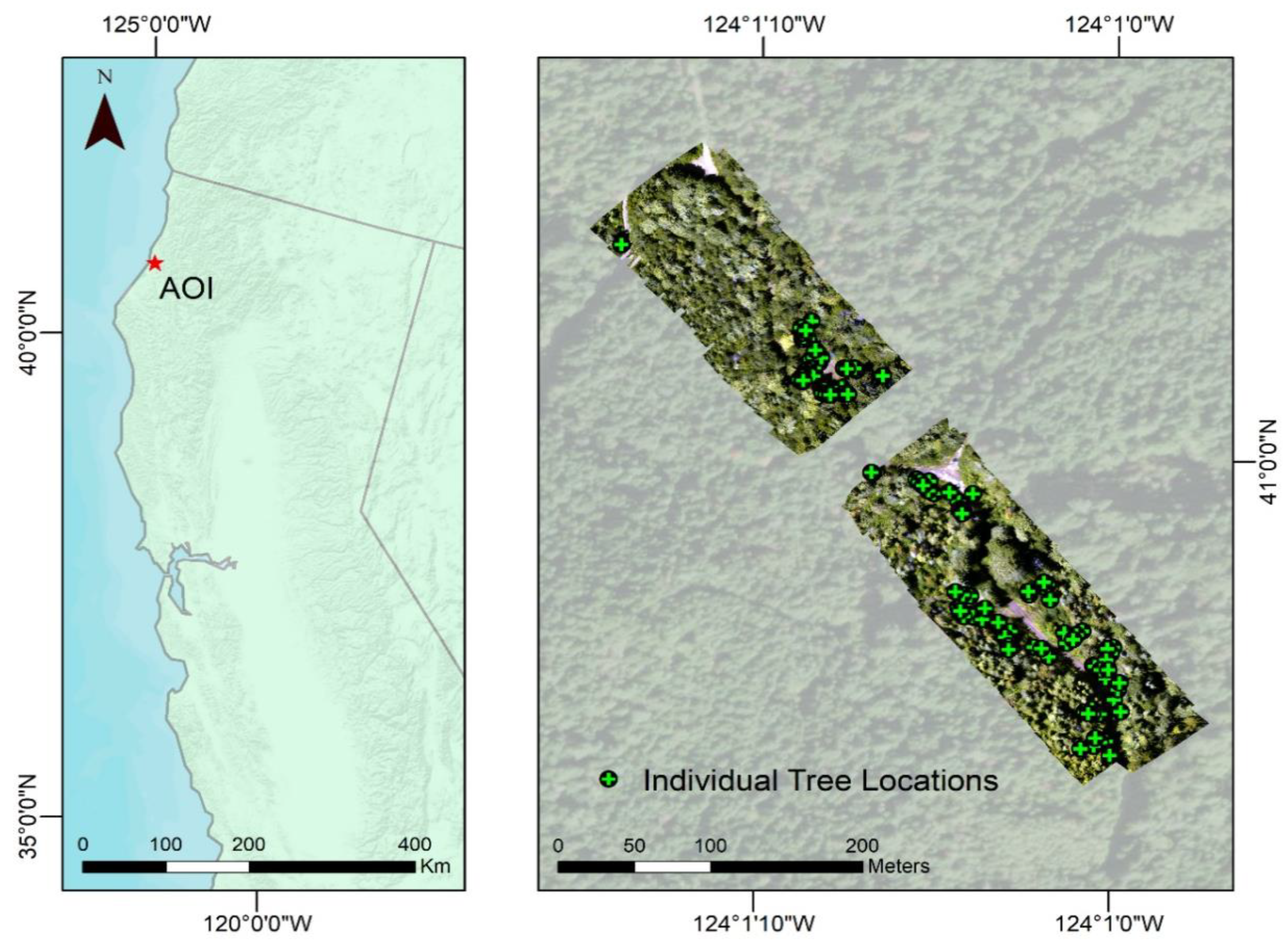
2.1. Site Location

The study was carried out in Humboldt County, California on land managed by the Green Diamond Resource Company. Initially, a larger property-wide search was carried out to identify a study area containing samples of healthy trees, trees with fresh damage, and trees with old damage. The area of interest (AOI), shown in Figure 1.
Identified (40.869652° N−123.964520° E) is a 515 m × 95 m (4.85 ha) strip that consists of a silvicultural mix of Redwood and Douglas-fir forests. This region of the Klamath Mountains is densely forested, containing some of the most productive timberlands in California. The climate geography of Northern California is greatly influenced by the ocean with moderate temperatures, an annual rainfall of 46 inches per year, and heavy fog throughout much of the year.

2.2. Experimental Design/Treatment Details

Trees were individually tagged, and tree health characteristics were noted early in the growing season. UAV based hyperspectral imagery was collected over the AOI, near the end of the growing season. Individual trees were located on the ground, to reference the aerial imagery. Crowns were manually digitized in a GIS, and the spectral information obtained within those tree crowns were organized into a data frame. Features (bands and indices) were then selected based on maximizing class separability among our three health classes. Using the results of the Jefferies-Matusita (JM) distance, a normalized channel ratio was developed among other commonly used indices to model tree health as a continuous variable 28. Various predictive classification models were developed, adding increasing combination of features. Model accuracy was assessed to determine the optimal model parameters needed for the image classification and to determine if there is enough statistical separation among our classes to make any recommendations for early stress identification. A workflow of the data collection and processing is shown in Figure 2.

2.3. Field Survey

Ground reference data of redwood trees that exhibited no damage, old damage, and fresh damage were collected in May and June of 2019. Training data collected in-situ were then categorized into three damage classes: trees with no damage, trees with fresh damage (<1 year), and trees with old damage (>1 year). Old damage was assumed to be any damage incurred before the present year and trees with recent damage were determined in the field. Trees with no damage were selected based on having no visible bark damage. Trees stripped within the year were identified by surveyor knowledge, with recently stripped trees being distinguishable from previously damaged trees (Figure 3). To determine in the field if the damage was recent or old, bark characteristics, such as moisture and rigidity were assessed. The cambium layer and inner bark of freshly damaged trees are noticeably more hydrated and lighter in appearance (Figure 4). Conversely, older damaged trees have sealed off their damaged tissue and were dryer to the touch and had a darker, weathered appearance (Figure 4). Older damaged bark was also more rigid, while newly damaged bark was more malleable. Trees were marked in the field using an aluminum tree tag with ID. Individual tree health, ID, age of damage, visual canopy, and trunk symptoms were noted and organized using the Survey123 mobile application within ArcGIS© 10.1 [35]. Tree-location measurements were conducted in September and October of 2019, after UAV data collection. To accurately map individual trees, several precise ground control points (GCPs) were surveyed at the study site using an Emlid REACH RS + RTK GNSS base station and rover at an accuracy of 1–5 cm. The GCPs were then used to geographically orient a Nikon NPL-322+P total station to triangulate coordinates for individual trees.

2.4. UAV Data Collection and Processing

UAV-based data collection was conducted on 31 July 2019. The weather and illumination conditions were sunny, clear, and windless during the flight collection. The hyperspectral imagery was captured in 56 individual strips using a Headwall Nano-Hyperspec sensor mounted on a DJI Matrice 600 Pro Hexacopter. A Headwall Nano-Hyperspec imaging sensor collects a hypercube with a spectral range of approximately 400–1000 nm in 273 discrete spectral bands. Equipment characteristics are shown in Table 1 RGB imagery was collected using an RGB camera mounted on a DJI Phantom 4 Pro and the mosaic was used as a high-resolution reference to calibrate the hyperspectral imagery. The RGB mosaic was generated using the photogrammetry software toolkit from Pix4D and ground reference data collected using an Emlid REACH RS+ RTK GNSS base station and rover. To align the hyperspectral imagery, an RGB file of each hyperspectral strip was generated and imported into QGIS along with the georeferenced RGB ortho images. This allowed for easy tiepoint placement using a smaller sized file. Tiepoints were created for each strip and then matched to the corresponding location in the georeferenced RGB. These tiepoints were placed on objects that were easily visible in both the hyperspectral and RGB images such as the tops of individual trees or the ends of branches. The tiepoints were placed in such a way as to reduce the mean distance error for the tiepoints between the hyperspectral and RGB data. The full spectral range hyperspectral files were then imported into QGIS and georeferenced using the created tiepoints from the RGB strips.

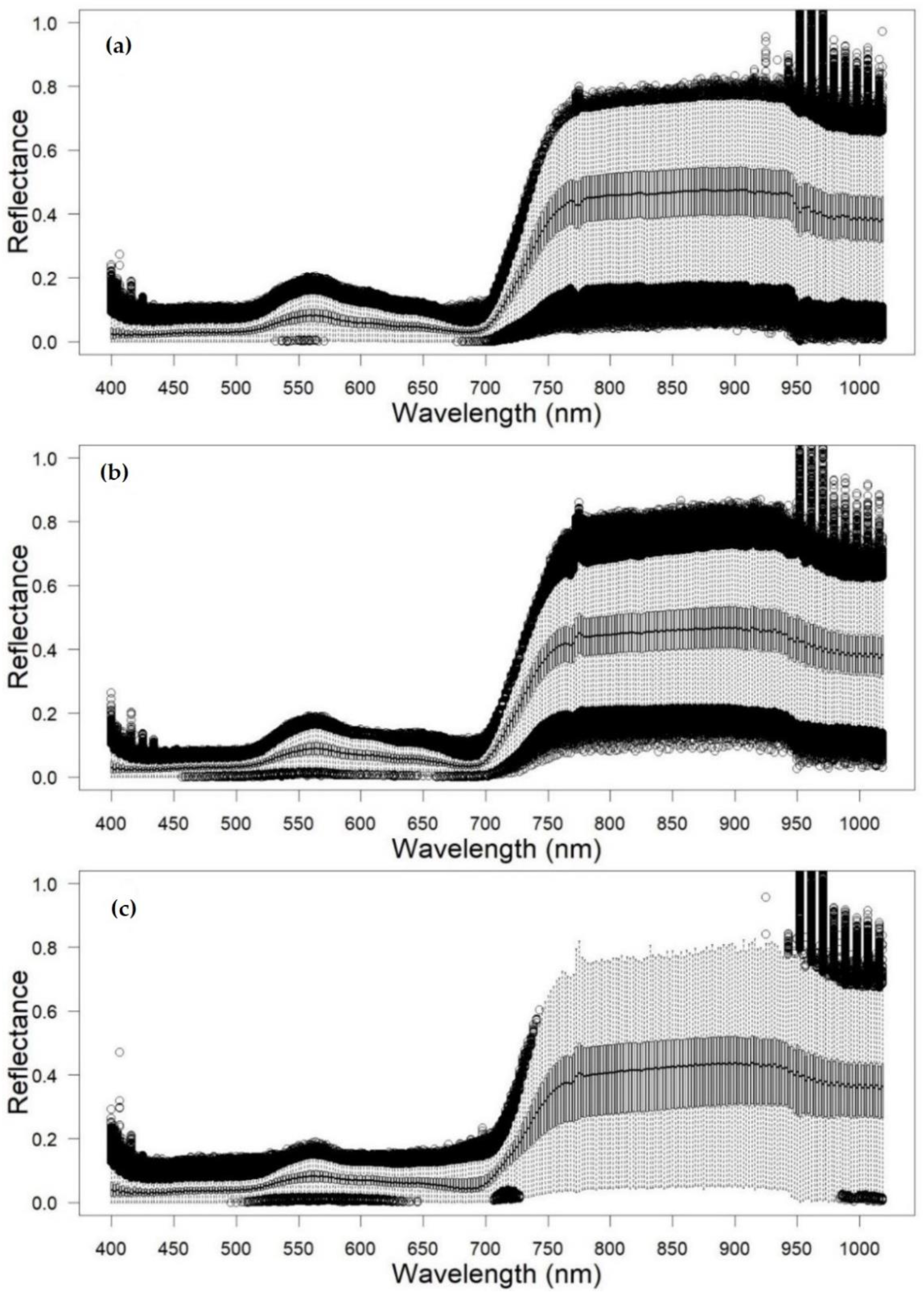
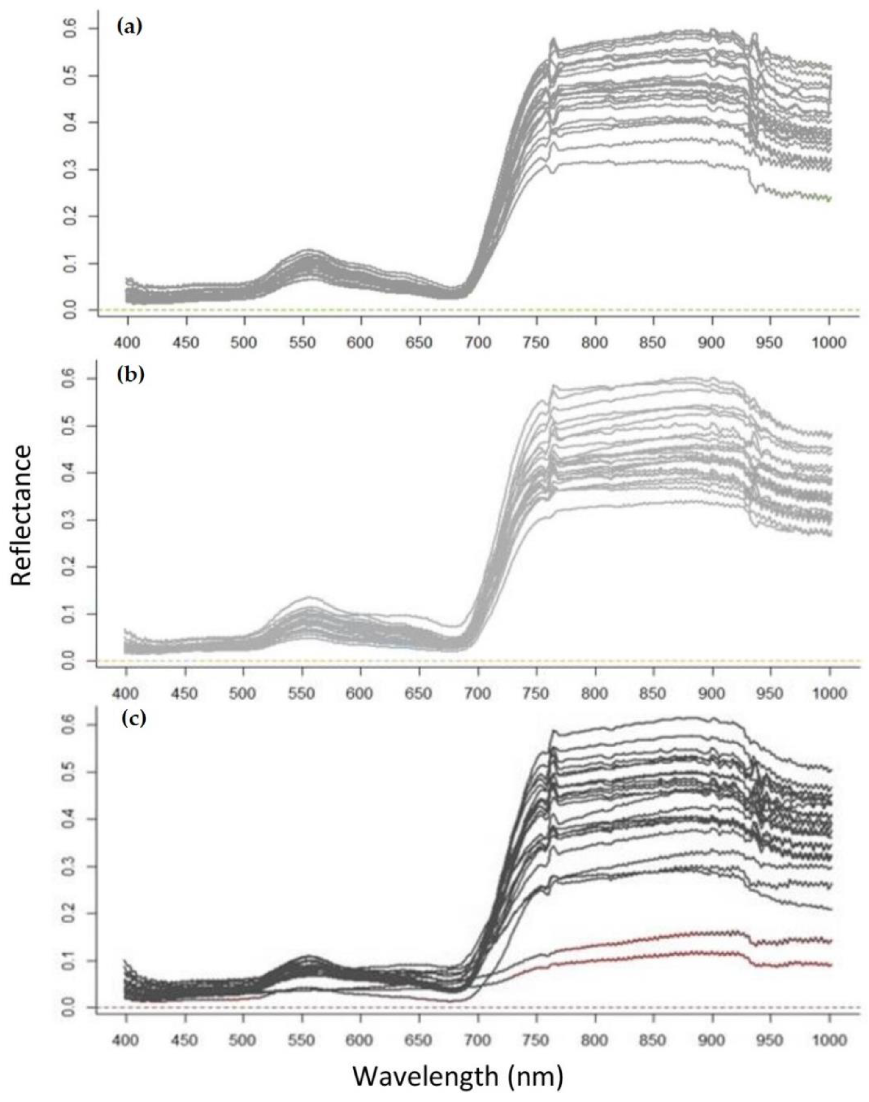
2.5. Crown Delineation and Spectral Signature Extraction

The imagery was captured from above, therefore it was important to select trees with canopies visible from above. Trees that were obstructed by adjacent canopies were removed from the sample. Locations of the field measured individual trees were identified by overlaying the point data on the hyperspectral imagery. Tree crowns were delineated manually using heads up digitizing and the resulting polygons were used as an extent to extract data values from the hyperspectral mosaic. A total of 108 trees belonging to the three health classes were delineated. This resulted in several thousand pixels related to each tree crown because of the high spatial resolution of the image data (i.e., ~2.5 cm/pixel). Information pertaining to tree crowns, pixels per tree crown, and total pixels per class are shown in Table 2. These extracted signatures were organized into a data frame for further analysis. A total of 368,958 signatures (pixels) across 273 bands, from 108 trees were used for feature selection (Figure 5).

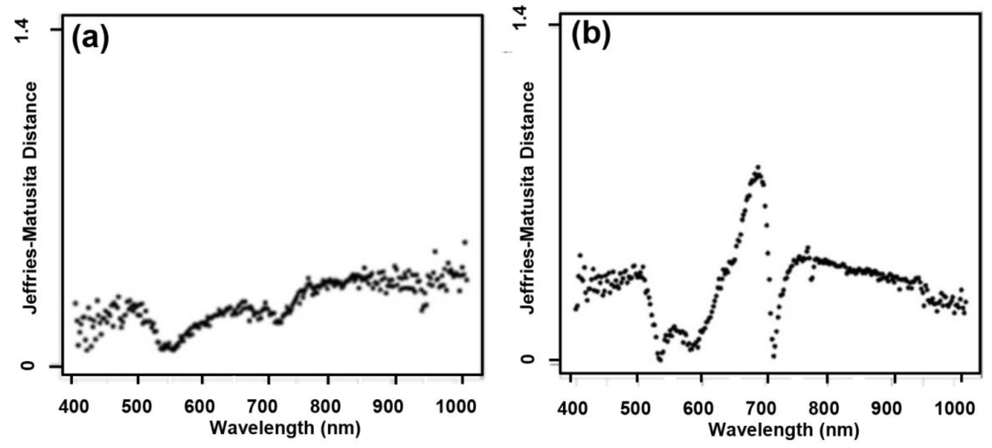
2.6. Feature Selection and Vegetation Indices Based on Class Separability

Feature selection is used to determine specific features or variables that maximize efficiency in machine learning models [36]. There are many reasons to employ feature selection techniques, the main premise being to identify redundant variables [36]. By removing irrelevant features, a subset of the data is used. This decreases training time and simplifies the model to avoid overfitting and ultimately the ‘curse of dimensionality’ [37]. To reduce the number of bands and limit redundancy in the model, optimal features which best demonstrate the separation among the three health classes were determined statistically. To quantify the split in the data among the three health classes across all hyperspectral bands, the Jeffries-Matusita (JM) statistic was used to determine the amount of overlap two distinct datasets are experiencing. The JM distance seeks to determine how entangled or split two distributions of data are and is commonly used in feature selection of hyperspectral data. This statistic was calculated at each of the 237 bands, using a binary, one vs. one approach [36] between the data extracted from healthy and freshly damaged trees and between the data extracted from healthy and old damaged trees. The JM distance is a statistical separability measurement which values range from 0 (no separability between the two distributions of data) to the square root of 2 (complete separability between the two distributions of data) [38]. A JM distance of the √2 implies the classification accuracy for that variable would be perfect between the two classes being compared because none of the data overlaps. A value below the √2 will have some level of uncertainty and some of the data between the two classes being compared are overlapping. A JM value of zero implies the distribution of the data between the two classes being compared is completely intersecting. The JM values were calculated for each class combination (healthy vs. fresh damage and healthy vs. old damage) against each spectral band to determine features with greater class separation. JM distance was employed to find specific band combinations maximizing the dissimilarity of the reflectance values for our three classes [36]. This information was used to create a series of commonly used indices and a normalized channel ratio capable of discerning class boundaries (Table 3).

2.7. Classification

The field data allowed for the calibration of our in-situ aerial data and our trees of interest on the ground. Different averaging methods were used to decide on the actual pixel values used for training (e.g., average or median of all pixels, or average or median of n number of brightest pixels within each tree extent) [17,42]. The average signature for each training tree was chosen and is shown in Figure 6. The vegetation indices calculated were also used as continuous features for model training. Classification models such as Support Vector Machines [43] and Random Forests [44] were tested to determine the optimal model to use in this classification.
The Support Vector Machine (SVM) learning approach is a supervised classification technique often used to classify data into two unique classes [45]. Published in 1963, SVM was primarily used to categorize classes based on values of linear combinations and characteristics of the data [46]. With the advent of computing power, SVMs have been implemented in remote sensing workflows for land classification applications [47,48,49]. SVMs use a kernel window to evaluate the general relationships in covariate datasets and define the margins among all classes [50]. SVMs use this kernel approach to define a hyperplane by splitting the data in covariate space where the separation in the individual classes of the dataset is maximized [49,51]. The relationship among the data is non-linear, therefore, the radial basis function was used as it has been shown to be the preferred function as demonstrated by Melgani and Bruzzone [51]. The tuning parameter required for the SVM function is cost. The maximum cost value for the radial based function is 1 and was chosen to minimize the training error in the model [52]. The SVM classifier has proven to be a successful land classification algorithm as it handles high dimensional feature spaces such as hyperspectral imagery, even when presented with small and imbalanced training datasets [51].
Random Forest (RF) is a decision tree ensemble method seeking to classify multi-class datasets [53]. This classifier builds many individual decision trees, using a branching decision process to limit the amount of variance in the predictive power [37]. Decision trees are built from a matrix of input feature covariates and categorical response variables. Several subsets of the matrix are created and structured using two parameters, k (number of trees) and n (number of branches). When determining the parameter values in the model, Rodriguez-Galiano et al. [54] demonstrated a decision forest with many trees (k) and a small number of branch nodes (n) will minimize the correlation among trees while reducing bias from complex training data. For this reason, the number of trees was held constant at 500 and the number of branch nodes was held constant at 2. RF uses a rational approach by combining several learning models to increase the accuracy of the classification, a method often called bagging [37]. For each decision tree of the random forest, a proportion of the data is used to build the tree and the remainder is used to validate the predicting capability of the tree [55]. After each tree in the forest has been built, the collective decision trees are used to make a prediction on the categorical outcome of the n-dimensional feature space, in this example the hyperspectral bands and indices. Random forest uses this bagging approach to average noisy models, creating a predictor with lower variance [56].

2.8. Accuracy Assessment

Using a K-fold cross validation approach, the data extracted from the tree crowns in the study site were classified and validated for accuracy, using a portion of the data to train the model and the remainder to test the model fit [57]. To validate the RF and SVM model, a ten-fold repeated cross-validation was implemented. The dataset was split using 90% of the data to train the model and 10% of the data to validate the accuracy of the model. This cross-validation approach was repeated ten times ensuring all data was used in the training and validating process. This was used to determine how well the model will generalize to an unknown dataset. To enable a better isolation of tree-tops, a pixel level classification was performed, so performance was determined by computing the ratio of correct to incorrect predictions and the kappa statistic. The approach using pixels was reported to provide better separation of the crown color classes in comparison to averaged spectra [18]. Accuracy was determined at the pixel level but also assessed visually at the tree crown level. The field data was compared to the highest performing model to assess performance across a stand rather than assessing pixel level classifications alone. All data processing was completed in the statistical package R, version 3.5.1 [58]. Model training and cross-validation was completed using the “caret” package [59].

3. Results

3.1. Feature Selection

Figure 7a illustrates the VNIR variable importance between healthy redwoods and freshly damage redwoods. In the visible range, there is a slight increase in separation among these two classes near 500 nm and 685 nm, and in the near-infrared portion, there is a slightly more distinct difference between the two health classes. Near 550 nm, a trend of nearly no distinction among the healthy and present damage classes is seen. There is no region in the VNIR where the JM distance between healthy and recently damaged canopies approaches √2, which would ensure classification. This implies the hyperspectral data between these two classes is overlapping. This likely inhibited classification of freshly damaged redwood trees because the spectral information is too similar. In Figure 7b, the JM criterion for the VNIR variables between the healthy and old damage class is shown. There is almost no distinction along the red-edge (~700 nm) indicating complete class overlap in that region. Just beyond the red edge, there is a slight increase in this statistic around 750 nm and a considerable difference near 685 nm, indicating the greatest class separation in the data between healthy redwoods and old damaged redwoods.
When comparing our tree health classes, there are no VNIR features that approaches √2, suggesting the data is too similar to enable an accurate classification (Figure 7).

3.2. Classification Accuracy

Table 4 shows the pixel-level OA and Kappa statistic for each of the feature datasets tested using the SVM and RF classifier. The most informative result was reached using VNIR features in an SVM model, with an OA of 83.8% and a kappa statistic of 0.75. None of the individual vegetation indices surpassed the accuracies attained using the VNIR features. Using all VIs improved model accuracy compared to using individual indices but was considerably less accurate than using the VNIR features. Performance decreased when using the full dataset which included the VNIR and VIs. For each feature set used, the SVM classifier outperformed the RF classifier in both OA and kappa.

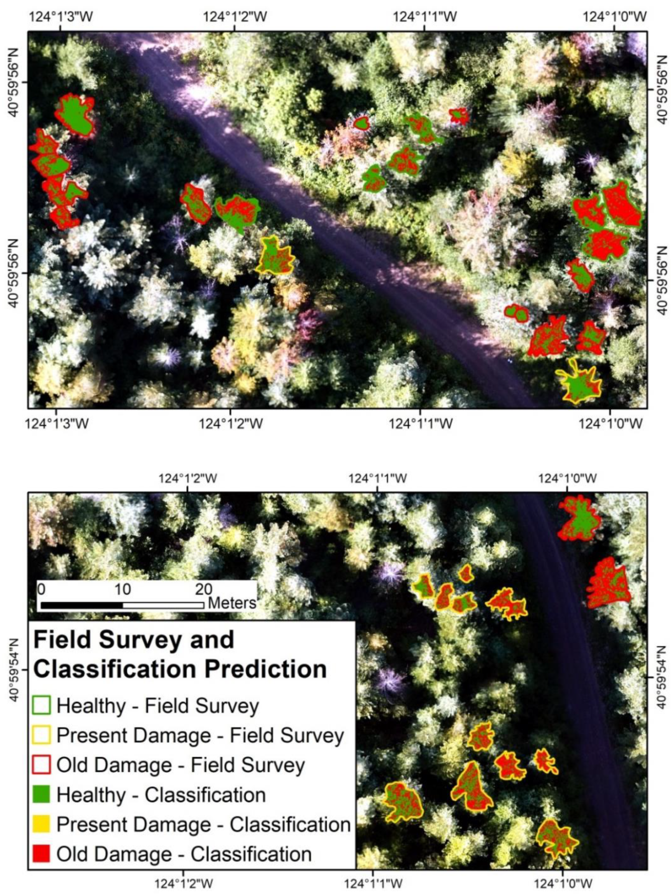
3.3. Model Prediction

Figure 8 shows two areas in the study site to compare the classification results to what was observed in the field. Due to the statistically similar and overlapping spectral signatures between the healthy and presently damaged class, the model struggled to predict trees in the early attack stage and generally classified those trees as healthy or old damage (Figure 8). Within individual tree crowns, the model often misclassified pixels or classified individual pixels within an individual tree crown into two classes, healthy and old damage, but rarely classified an entire tree crown as one class. Spectrally, healthy, and presently damaged classes were too similar to distinguish using the hyperspectral imagery.

4. Discussion

4.1. Redwood Tree Characteristics

The main challenge to validate in this study was the assumption that damage to each redwood tree was sustained simultaneously. Bears will select groups of trees but unlike other pests, e.g., bark beetles, will target trees over several weeks to months. Therefore, the training trees in the model did not incur damage at the same rate, thus some trees may have had a longer period to show signs of stress in the canopy layer. Several studies have examined the intraspecies spectral variability of health and damaged trees in a variety of applications (i.e., albeit focusing on bark beetles) [17] with the main assumption being that the infected trees senesce similarly. In this study, however, it was difficult to validate this assumption since the timing of redwood trees being damaged and the resulting effect on the tree canopy varied due to the independent and isolated nature of this disturbance.
Unlike Douglas-fir, which are also susceptible to black bear bark stripping attack, redwoods have a unique ability to recover from these disturbances. Some trees that were attacked were able to recover with no visible signs of damage, whereas other attacked trees were unable to recover and showed signs of early senescence. Unlike other forest disturbances, such as bark beetle, there is not necessarily a high mortality rate, but the damage incurred likely only slowed the trees growth as it heals itself. With bark beetle outbreaks, if a tree is infested, the tree will likely perish and the timing is fairly uniform across the stand [16]. Bear bark stripping occurs over several months and is patchy in nature. Trees may only be partially girdled, especially near the bottom which adds inherent complexity to the model.

4.2. Feature Selection, Variable Importance and Early Detection of Damage

This study was implemented to determine the possibility of discerning healthy and recently attacked redwood trees using hyperspectral imagery acquired from a UAV platform. Several studies have explored the use of hyperspectral imagery to estimate chlorophyll content, which is used as a proxy for tree health [19,60,61,62]. Abundant chlorophyll pigments of healthy plant leaves are responsible for photosynthesis, playing a major role in the absorption of light in the red and blue wavelengths, and its reflection in the Near-infrared (NIR) portion of the electromagnetic spectrum [63]. Several months after the bear bark stripping event, completely girdled redwood tree canopies may begin to turn yellow, then red, and then finally grey as the chlorophyll content degrades, revealing the leaf carotenoids and resulting in senescence [19]. Partially girdled trees often recover and may show no signs of stress, making them undetectable, but will experience decreased growth rates and increased susceptibility to various fungal diseases [6]. When a tree is stressed, the leaf surface reflectance in the blue, green, and red regions of the visible (VIS) portion increases while decreasing in the NIR wavelengths [19,64]. This stress-induced increase of reflectance in the VIS interval is most observed between the red and red edge region (650–700 nm) making it a critical range for early detection of vegetation stress, and thus a focus for early forest damage detection [65]. This trend was noticeable in this study, but only between healthy and old damaged redwood trees (Figure 7). Among our two classes of interest, healthy and recently damaged, the JM distances did not show importance among the band indices, suggesting the need to extend the recent damage window. This also suggests the spectral overlap among our health classes is significant enough, thus creating model uncertainty and confusion.

4.3. UAV-Based Image Acquisition in Forest Health Monitoring

Imagery collected using UAV technology is showing promise in providing similar metrics to traditional on-the-ground sampling methods seeking to monitor forest health [15,17,66]. The use of UAVs to monitor forest health does have its set of strengths and limitations. With the ability to control flight height, spatial resolution is greatly increased. This detail is helpful when examining forest characteristics at the individual tree level, but the tradeoff with increased spatial resolution is limited spatial extent making UAVs useful for targeted monitoring limited to small areas or stands. Field methods of detecting bear bark stripping are laborious and time-consuming [12,67]. Remote sensing technology offers the ability to estimate vegetation health with precision and detail, and the above ground nature of the data allows for the assessment of anomalies in crown health over extensive areas at varying spatial and temporal scales. Remote sensing of forest health has largely focused on insect infestations using a wide range of datasets, including passive multispectral imagery, synthetic aperture radar, lidar [24,42,65,68,69,70], and at moderate to coarse scale using pixel level approaches [26,70]. However, bear bark stripping occurs on single, isolated trees or small clusters of trees even when generally associated with linear features such as roads or trails, or broad scale drainage areas [6]. As such, high spatial resolution remote sensing data and methods capable of single tree detection are crucial for identifying bear bark stripping at the finest scale to develop more accurate upscaled models.
Presently, no studies have examined bear damage using UAV acquired data, but similar approaches have been demonstrated in applications such as monitoring bark beetle outbreaks [17,18]. Researchers utilized UAV-based high-resolution hyperspectral image data to assess bark beetle infestation in Norway spruce (Picea abies L.) in Finland [17]. The study identified different stages of health (i.e., healthy, infested, and dead trees) using machine vision technologies with an overall accuracy of 76% when using three classes (healthy, infested, and dead) and 90% when using only two classes (healthy and dead) [17]. This same study was later expanded upon, to compare the high-resolution UAV data to moderate resolution aircraft data using a variety of vegetation indices and reported a best overall accuracy of 73% (Kappa 0.56) with aircraft data compared to a best overall accuracy of 81% (Kappa 0.7) with the UAV data for the above mentioned three classes [18]. There are few studies in this area of forest health monitoring, but the encouraging results shown in these examples demonstrate novel, low-cost remote sensing technologies offer a great potential for affordable and timely assessments of tree health condition.
Recent advancements in UAV technology have opened a new scientific endeavor, offering novel data collection approaches with lower operating costs than manned aircraft data acquisition systems [71]. UAVs can be flown at much lower altitudes and over narrow time intervals, capturing ultra-high spatial and temporal resolution data [72]. With this gain in spatial and spectral resolution, tree-level redwood variation can be analyzed more effectively over larger spatial extents [68]. Collecting spectral data using UAVs verified the advantages of this method of image acquisition [22]. The benefit of using hyperspectral sensors is the increased spectral resolution, providing a more detailed data cube capable of discerning marginal changes in intraspecies variation. The use of hyperspectral bands to classify diverse landscapes at the species level has been demonstrated with promising results [25]. In this study, however, intraspecies spectral variation was for only one tree species, the redwood. The main question being asked was whether trees with recent damage could be detected and isolated among healthy trees. The capabilities of UAVs in remote sensing workflows will likely improve, with the advent of computing power and UAV technology, but in this example detecting trees with recent damage could not be achieved.

5. Conclusions

This study explored the capacity of UAV-based hyperspectral imaging to identify redwood trees in the early attack stage of senescence. The results showed there is little distinction between healthy redwoods and presently damaged redwoods in the four-month window between survey and image collection suggesting the time allotted in this experiment may be insufficient to see a response in the canopy via remote sensing. One benefit of UAVs is the increase temporal resolution. Going forward, it would be of interest to model this disturbance over time to develop a better understanding of the timing of senescence and the effect this disturbance has on growth and recovery rates. Bear bark stripping is a particularly common and puzzling disturbance in redwood forests of Northern California, occurring in seemingly random patches and irregular time intervals. Although it is unclear what causes bears to target the cambium layer of certain trees as a food source, developing methods to identify individual trees and ultimately identify the spatial patterns of this disturbance may aid future research in understanding the fundamental link driving this behavior. An understanding of the spatial patterns of bear bark stripped trees is a critical step in identifying the causes and possible solutions to this wildlife-forest interaction. If identified correctly, patterns of damaged trees can be used to customize harvesting operations. High-resolution data may be the link to spatially optimizing land use, accommodating both timber production and habitat preservation. In the long term, the products of this research will contribute to more efficient and sustainable forest management, by helping to identify early tree stress at a landscape level.

Author Contributions

Conceptualization, S.M., D.G., B.M.; methodology, S.M.; software, S.M.; validation, S.M.; formal analysis, S.M.; investigation, S.M., D.G.; writing—S.M., writing—review and editing, S.M., D.G., B.M.; visualization, S.M.; supervision, D.G., B.M.; project administration, D.G., B.M. All authors have read and agreed to the published version of the manuscript.

Funding

This research was funded by Agricultural Research Institute, grant number S04106 and GI 2025 funds from HSU CNRS program. The APC was waived for Buddhika Madurapperuma, who was the winner for Outstanding Reviewer Awards 2019.

Data Availability Statement

Data sharing not applicable.

Acknowledgments

The authors wish to thank Green Diamond Resource Company for providing access to the premises for conducting this research. We also want to thank Asinn Kim for assistance with the field survey and data analysis.

Conflicts of Interest

The authors declare no conflict of interest.

References

  1. Sillett, S.C.; Van Pelt, R.; Carroll, A.L.; Kramer, R.D.; Ambrose, A.R.; Trask, D. How do tree structure and old age affect growth potential of California redwoods? Ecol. Monogr. 2015, 85, 181–212. [Google Scholar] [CrossRef]
  2. Brown, C. Habitat Use and Movement Patterns of Two Redwood Forest Salamanders, Aneides Vagrans and Ensatina Eschscholtzii, with an Examination of the Efficacy of Pit Tags for Marking Small Plethodontids; Humboldt State University: Arcata, CA, USA, 2017. [Google Scholar]
  3. Fish, U.S.; Service, W. Endangered and Threatened Wildlife and Plants: Determination of Threatened Status for the Northern Spotted Owl. Fed. Regist. 1990, 55, 26114–26194. [Google Scholar]
  4. Lorimer, C.G.; Porter, D.J.; Madej, M.A.; Stuart, J.D.; Veirs, S.D., Jr.; Norman, S.P.; O’Hara, K.L.; Libby, W.J. Presettlement and modern disturbance regimes in coast redwood forests: Implications for the conservation of old-growth stands. For. Ecol. Manag. 2009, 258, 1038–1054. [Google Scholar] [CrossRef]
  5. Ziegltrum, G. Cost-Effectiveness of the Black Bear Supplemental Feeding Program in Western Washington. Wildife Soc. Bull. 2006, 34, 375–379. [Google Scholar] [CrossRef]
  6. Giusti, G. Recognizing Damage by Black Bear Damage to Second Growth Redwoods. In Proceedings of the 13th Vertebrate Pest Conference, Monterey, CA, USA, 1–3 March 1988. [Google Scholar]
  7. Giusti, G. UC Agriculture & Natural Resources Proceedings of the Vertebrate Pest Conference. In Proceedings of the Vertebrate Pest Conference, Sacramento, CA, USA, 6–8 March 1990. [Google Scholar]
  8. Glover, F. Glover Source. J. Wildl. Manag. 1955, 19, 437–443. [Google Scholar] [CrossRef]
  9. Matthews, S.M.; Golightly, R.T.; Higley, J.M. Mark–resight density estimation for American black bears in Hoopa, California. Ursus 2008, 19, 13–21. [Google Scholar] [CrossRef]
  10. Ziegltrum, G.J. Efficacy of black bear supplemental feeding to reduce conifer damage in western washington. J. Wildl. Manag. 2004, 68, 470–474. [Google Scholar] [CrossRef] [Green Version]
  11. Kanaskie, A.; Chetock, J.; Irwin, G.; Overhusler, D. Black Bear Damage to Forest Trees in Northwest Oregon 1988–1989. Pest Manag. Rep. 1990, 90, 34p. [Google Scholar]
  12. Taylor, J.D.; Kline, K.N.; Morzillo, A.T. Estimating economic impact of black bear damage to western conifers at a landscape scale. For. Ecol. Manag. 2019, 432, 599–606. [Google Scholar] [CrossRef] [Green Version]
  13. Nolte, D.L.; Dykzeul, M. Wildlife Impacts on Forest Resources. Hum. Confl. Wildl. Econ. Consid. 2000, 20, 163–168. [Google Scholar]
  14. Panigrahy, S.; Kumar, T.; Manjunath, K.R. Hyperspectral leaf signature as an added dimension for species discrimination: Case study of four tropical mangroves. Wetl. Ecol. Manag. 2012, 20, 101–110. [Google Scholar] [CrossRef]
  15. Foster, A.C.; Walter, J.A.; Shugart, H.H.; Sibold, J.; Negron, J. Spectral evidence of early-stage spruce beetle infestation in Engelmann spruce. For. Ecol. Manag. 2017, 384, 347–357. [Google Scholar] [CrossRef] [Green Version]
  16. Hall, R.; Castilla, G.; White, J.; Cooke, B.; Skakun, R. Remote sensing of forest pest damage: A review and lessons learned from a Canadian perspective. Can. Èntomol. 2016, 148, S296–S356. [Google Scholar] [CrossRef]
  17. Näsi, R.; Honkavaara, E.; Lyytikäinen-Saarenmaa, P.; Blomqvist, M.; Litkey, P.; Hakala, T.; Viljanen, N.; Kantola, T.; Tanhuanpää, T.; Holopainen, M. Using UAV-Based Photogrammetry and Hyperspectral Imaging for Mapping Bark Beetle Damage at Tree-Level. Remote Sens. 2015, 7, 15467–15493. [Google Scholar] [CrossRef] [Green Version]
  18. Näsi, R.; Honkavaara, E.; Blomqvist, M.; Lyytikäinen-Saarenmaa, P.; Hakala, T.; Viljanen, N.; Kantola, T.; Holopainen, M. Remote sensing of bark beetle damage in urban forests at individual tree level using a novel hyperspectral camera from UAV and aircraft. Urban For. Urban Green. 2018, 30, 72–83. [Google Scholar] [CrossRef]
  19. Carter, G.A. Carter Source. Am. J. Bot. 1993, 80, 239–243. [Google Scholar] [CrossRef]
  20. Vogelmann, J.E.; Rock, B.N.; Moss, D.M. Red edge spectral measurements from sugar maple leaves. Int. J. Remote Sens. 1993, 14, 1563–1575. [Google Scholar] [CrossRef]
  21. Merzlyak, M.N.; Gitelson, A.A.; Chivkunova, O.B.; Rakitin, V.Y. Non-destructive optical detection of pigment changes during leaf senescence and fruit ripening. Physiol. Plant. 1999, 106, 135–141. [Google Scholar] [CrossRef] [Green Version]
  22. Dash, J.P.; Watt, M.S.; Pearse, G.D.; Heaphy, M.; Dungey, H.S. Assessing very high resolution UAV imagery for monitoring forest health during a simulated disease outbreak. ISPRS J. Photogramm. Remote Sens. 2017, 131, 1–14. [Google Scholar] [CrossRef]
  23. Adam, E.; Mutanga, O.; Rugege, D. Multispectral and hyperspectral remote sensing for identification and mapping of wetland vegetation: A review. Wetl. Ecol. Manag. 2010, 18, 281–296. [Google Scholar] [CrossRef]
  24. Ortiz, S.; Breidenbach, J.; Kändler, G. Early Detection of Bark Beetle Green Attack Using TerraSAR-X and RapidEye Data. Remote Sens. 2013, 5, 1912–1931. [Google Scholar] [CrossRef] [Green Version]
  25. Sothe, C.; Dalponte, M.; De Almeida, C.M.; Schimalski, M.B.; Lima, C.L.; Liesenberg, V.; Miyoshi, G.T.; Tommaselli, A.M.G. Tree Species Classification in a Highly Diverse Subtropical Forest Integrating UAV-Based Photogrammetric Point Cloud and Hyperspectral Data. Remote Sens. 2019, 11, 1338. [Google Scholar] [CrossRef] [Green Version]
  26. Coops, N.C.; Waring, R.H.; Wulder, M.A.; White, J.C. Prediction and assessment of bark beetle-induced mortality of lodgepole pine using estimates of stand vigor derived from remotely sensed data. Remote Sens. Environ. 2009, 113, 1058–1066. [Google Scholar] [CrossRef]
  27. Turner, D.; Lucieer, A.; Watson, C. Development of an Unmanned Aerial Vehicle (UAV) for Hyper Resolution Vineyard Mapping Based on Visible, Multispectral, and Thermal Imagery. In Proceedings of the 34th International Symposium on Remote Sensing of Environment, Sydney, Australia, 10–15 April 2011. [Google Scholar]
  28. Maschler, J.; Atzberger, C.; Immitzer, M. Individual Tree Crown Segmentation and Classification of 13 Tree Species Using Airborne Hyperspectral Data. Remote Sens. 2018, 10, 1218. [Google Scholar] [CrossRef] [Green Version]
  29. Alonzo, M.; Roth, K.; Roberts, D. Identifying Santa Barbara’s urban tree species from AVIRIS imagery using canonical discriminant analysis. Remote Sens. Lett. 2013, 4, 513–521. [Google Scholar] [CrossRef]
  30. Alonzo, M.; Bookhagen, B.; Roberts, D.A. Urban tree species mapping using hyperspectral and lidar data fusion. Remote Sens. Environ. 2014, 148, 70–83. [Google Scholar] [CrossRef]
  31. Bunting, P.; Lucas, R. The delineation of tree crowns in Australian mixed species forests using hyperspectral Compact Airborne Spectrographic Imager (CASI) data. Remote Sens. Environ. 2006, 101, 230–248. [Google Scholar] [CrossRef]
  32. Zarco-Tejada, P.; Hornero, A.; Hernández-Clemente, R.; Beck, P. Understanding the temporal dimension of the red-edge spectral region for forest decline detection using high-resolution hyperspectral and Sentinel-2a imagery. ISPRS J. Photogramm. Remote Sens. 2018, 137, 134–148. [Google Scholar] [CrossRef]
  33. Degerickx, J.; Roberts, D.; McFadden, J.; Hermy, M.; Somers, B. Urban tree health assessment using airborne hyperspectral and LiDAR imagery. Int. J. Appl. Earth Obs. Geoinf. 2018, 73, 26–38. [Google Scholar] [CrossRef] [Green Version]
  34. Lowe, A.; Harrison, N.; French, A.P. Hyperspectral image analysis techniques for the detection and classification of the early onset of plant disease and stress. Plant Methods 2017, 13, 1–12. [Google Scholar] [CrossRef]
  35. Esri, A. ArcGIS 10.1; ESRI Inc.: Redlands, CA, USA, 2012. [Google Scholar]
  36. Bruzzone, L.; Roli, F.; Serpico, S. An extension of the Jeffreys-Matusita distance to multiclass cases for feature selection. IEEE Trans. Geosci. Remote Sens. 1995, 33, 1318–1321. [Google Scholar] [CrossRef] [Green Version]
  37. Belgiu, M.; Drăguţ, L. Random forest in remote sensing: A review of applications and future directions. ISPRS J. Photogramm. Remote Sens. 2016, 114, 24–31. [Google Scholar] [CrossRef]
  38. Medjahed, S.; Saadi, T.A.; Benyettou, A.; Ouali, M. Gray Wolf Optimizer for hyperspectral band selection. Appl. Soft Comput. 2016, 40, 178–186. [Google Scholar] [CrossRef]
  39. Rouse, J.W., Jr.; Haas, R.H.; Schell, J.A.; Deering, D.W. Paper A 20. In Third Earth Resources Technology Satellite-1 Symposium: The Proceedings of a Symposium Held by Goddard Space Flight Center at Washington, DC on 10–14 December 1973; Goddard Space Flight Center: Greenbelt, MD, USA, 1974; Volume 351, p. 309. [Google Scholar]
  40. Daughtry, C.S.T.; Walthall, C.L.; Kim, M.S.; De Colstoun, E.B.; McMurtrey, J.E., III. Estimating Corn Leaf Chlorophyll Concentration from Leaf and Canopy Reflectance. Remote Sens. Environ. 2000, 74, 229–239. [Google Scholar] [CrossRef]
  41. Vogelmann, J.E. Comparison between two vegetation indices for measuring different types of forest damage in the north-eastern United States. Int. J. Remote Sens. 1990, 11, 2281–2297. [Google Scholar] [CrossRef]
  42. Kantola, T.; Vastaranta, M.; Lyytikäinen-Saarenmaa, P.; Holopainen, M.; Kankare, V.; Talvitie, M.; Hyyppa, J. Classification of Needle Loss of Individual Scots Pine Trees by Means of Airborne Laser Scanning. Forest 2013, 4, 386–403. [Google Scholar] [CrossRef] [Green Version]
  43. Chang, C.-C.; Lin, C.-J. LIBSVM: A Library for Support Vector Machines. ACM Trans. Intell. Syst. Technol. 2011, 2, 27. [Google Scholar] [CrossRef]
  44. Breiman, L. Random Forests. J. Electrochem. Soc. 1999, 129, 2865. [Google Scholar]
  45. Cortes, C.; Vapnik, V. Support-Vector Networks. Mach. Learn. 1995, 20, 273–297. [Google Scholar] [CrossRef]
  46. Vapnik, V. Pattern Recognition Using Generalized Portrait Method. Autom. Remote Control 1963, 24, 774–780. [Google Scholar]
  47. Ebrahimi, M.; Khoshtaghaza, M.; Minaei, S.; Jamshidi, B. Vision-based pest detection based on SVM classification method. Comput. Electron. Agric. 2017, 137, 52–58. [Google Scholar] [CrossRef]
  48. Gualtieri, J.A. The Support Vector Machine (SVM) Algorithm for Supervised Classification of Hyperspectral Remote Sensing Data. Kernel Methods Remote Sens. Data Anal. 2009, 3, 49–83. [Google Scholar] [CrossRef]
  49. Hsu, C.-W.; Chang, C.-C.; Lin, C.-J. A Practical Guide to SVM Classification. 2003. Available online: http//www.csie.ntu.edu.tw/~cjlin/papers/guide/guide.pdf (accessed on 6 December 2019).
  50. Tzotsos, A.; Argialas, D.P. Support Vector Machine Classification for Object-Based Image Analysis. In Lecture Notes in Geoinformation and Cartography; Springer: Berlin/Heidelberg, Germany, 2008; pp. 663–677. [Google Scholar]
  51. Melgani, F.; Bruzzone, L. Classification of hyperspectral remote sensing images with support vector machines. IEEE Trans. Geosci. Remote Sens. 2004, 42, 1778–1790. [Google Scholar] [CrossRef] [Green Version]
  52. Joachims, T. Optimizing Search Engines Using Clickthrough Data. In Proceedings of the Eighth ACM SIGKDD International Conference on Knowledge Discovery and Data Mining, Edmonton, AB, USA, 23–26 July 2002; pp. 133–142. [Google Scholar]
  53. Gall, J.; Yao, A.; Razavi, N.; Van Gool, L.; Lempitsky, V. Hough Forests for Object Detection, Tracking, and Action Recognition. IEEE Trans. Pattern Anal. Mach. Intell. 2011, 33, 2188–2202. [Google Scholar] [CrossRef]
  54. Rodriguez-Galiano, V.; Ghimire, B.; Rogan, J.; Chica-Olmo, M.; Rigol-Sanchez, J. An assessment of the effectiveness of a random forest classifier for land-cover classification. ISPRS J. Photogramm. Remote Sens. 2012, 67, 93–104. [Google Scholar] [CrossRef]
  55. Chan, J.C.-W.; Paelinckx, D. Evaluation of Random Forest and Adaboost tree-based ensemble classification and spectral band selection for ecotope mapping using airborne hyperspectral imagery. Remote Sens. Environ. 2008, 112, 2999–3011. [Google Scholar] [CrossRef]
  56. Gislason, P.O.; Benediktsson, J.A.; Sveinsson, J.R. Random Forests for land cover classification. Pattern Recognit. Lett. 2006, 27, 294–300. [Google Scholar] [CrossRef]
  57. Metropolis, N.; Ulam, S. The Monte Carlo Method. J. Am. Stat. Assoc. 1949, 44, 335–341. [Google Scholar] [CrossRef]
  58. Team, R.C. R: A Language and Environment for Statistical Computing; R Core Team: Vienna, Austria, 2013. [Google Scholar]
  59. Kuhn, V.I.; Ranson, K.J.; Fedotova, E.V. Building Predictive Models in R Using the Caret Package. J. Stat. Softw. 2008, 28, 1–26. [Google Scholar] [CrossRef] [Green Version]
  60. Gates, D.M.; Keegan, H.J.; Schleter, J.C.; Weidner, V.R. Spectral Properties of Plants. Appl. Opt. 1965, 4, 11–20. [Google Scholar] [CrossRef]
  61. Haboudane, D.; Miller, J.R.; Pattey, E.; Zarco-Tejada, P.J.; Strachan, I.B. Hyperspectral Vegetation Indices and Novel Algorithms for Predicting Green LAI of Crop Canopies: Modeling and Validation in the Context of Precision Agriculture. Remote Sens. Environ. 2004, 90, 337–352. [Google Scholar] [CrossRef]
  62. Knipling, E.B. Physical and physiological basis for the reflectance of visible and near-infrared radiation from vegetation. Remote Sens. Environ. 1970, 1, 155–159. [Google Scholar] [CrossRef]
  63. Mackinney, G. ABSORPTION OF LIGHT BY CHLOROPHYLL SOLUTIONS. J. Biol. Chem. 1941, 140, 315–322. [Google Scholar] [CrossRef]
  64. Carter, G.A.; Cibula, W.G.; Miller, R.L. Narrow-band Reflectance Imagery Compared with ThermalImagery for Early Detection of Plant Stress. J. Plant Physiol. 1996, 148, 515–522. [Google Scholar] [CrossRef]
  65. Rullan-Silva, C.; Olthoff, A.; De La Mata, J.D.; Pajares-Alonso, J. Remote Monitoring of Forest Insect Defoliation -A Review-. For. Syst. 2013, 22, 377–391. [Google Scholar] [CrossRef] [Green Version]
  66. Lehmann, J.R.K.; Nieberding, F.; Prinz, T.; Knoth, C. Analysis of Unmanned Aerial System-Based CIR Images in Forestry—A New Perspective to Monitor Pest Infestation Levels. Forest 2015, 6, 594–612. [Google Scholar] [CrossRef] [Green Version]
  67. Kanaskie, A.; Mcwilliams, M.; Overhulser, D.; Christian, R. Black Bear Damage to Forest Trees in Northwest Oregon: Aerial and Ground Surveys, 2000. Oregon Dep. For. Pest Manag. Rep 2001, 28, 1–29. [Google Scholar]
  68. Fassnacht, F.E.; Latifi, H.; Stereńczak, K.; Modzelewska, A.; Lefsky, M.; Waser, L.T.; Straub, C.; Ghosh, A. Review of studies on tree species classification from remotely sensed data. Remote Sens. Environ. 2016, 186, 64–87. [Google Scholar] [CrossRef]
  69. Kharuk, V.I.; Ranson, K.J.; Fedotova, E.V. Spatial pattern of Siberian silkmoth outbreak and taiga mortality. Scand. J. For. Res. 2007, 22, 531–536. [Google Scholar] [CrossRef]
  70. Wulder, M.; White, J.; Bentz, B.; Alvarez, M.; Coops, N. Estimating the probability of mountain pine beetle red-attack damage. Remote Sens. Environ. 2006, 101, 150–166. [Google Scholar] [CrossRef]
  71. Zhang, C.; Kovacs, J.M. The application of small unmanned aerial systems for precision agriculture: A review. Precis. Agric. 2012, 13, 693–712. [Google Scholar] [CrossRef]
  72. Aasen, H.; Honkavaara, E.; Lucieer, A.; Zarco-Tejada, P.J. Quantitative Remote Sensing at Ultra-High Resolution with UAV Spectroscopy: A Review of Sensor Technology, Measurement Procedures, and Data Correction Workflows. Remote Sens. 2018, 10, 1091. [Google Scholar] [CrossRef] [Green Version]
Figure 1. The area of interest (AOI) located in Humboldt County in Northern California. The extent of the hyperspectral imagery is shown on the right totaling 4.85 ha and the individual trees used to train the models.
Forests 12 00378 g001
Figure 2. Workflow of data analysis in this study.
Forests 12 00378 g002
Figure 3. An example of fresh damage observed in the field: (a) A redwood tree completely girdled by a black bear; (b) A redwood tree with half of the bark removed from the trunk.
Forests 12 00378 g003
Figure 4. An example of characteristics used to determine fresh damaged observed in the field: (a) A photo of bark from old damage (left) and fresh damage (right); (b) A tagged redwood tree with fresh damage.
Forests 12 00378 g004
Figure 5. A boxplot visualization of the spectral signatures extracted from the three classes: healthy tree (a), fresh damage (b), and old damage (c). The minimum quartile (0th percentile), the maximum quartile (100th percentile), the first quartile (25th percentile), and the third quartile (75th percentile), and the median (50th percentile) are shown as well as outliers (circles) for each class at each hyperspectral band.
Forests 12 00378 g005
Figure 6. The mean spectral signatures of each sample tree used as training: healthy class (a), fresh damage (b), and old damage (c).
Forests 12 00378 g006
Figure 7. The Jeffries-Matusita distance measure for each of the 273 spectral bands (400 nm to 1000 nm): (a) JM measure between healthy class and freshly damage class; (b) JM measure between healthy class and old damage class.
Forests 12 00378 g007
Figure 8. Comparing field observations (outline) to the tree health class prediction determined using the SVM classifier (pixel).
Forests 12 00378 g008
Table 1. Camera and flight characteristics of the equipment used in the study.
Imaging SensorHeadwall Nano-Hyperspec
Spectral bands273 spectral bands from 398 to 1001 nm
Focal Length4.8 mm
FWHM6 nm
Bit depth12-bit
Spatial bands640
Ground sampling distance (GSD)2.5 cm
Flight height90 m
Flight speed4 m/s
Table 2. Damage class for sample redwood trees, the total number of pixels, the number of individual tree crowns (ITCs), and the average number of pixels per individual tree crown.
IDDamage ClassITCsPixelsPixels/ITC
1No stress 45188,7524194
2Fresh Damage 12568,6952747
3Old Damage38111,6072937
1 Damage incurred within the month of survey.
Table 3. Vegetation indices used in this study and the equation used to generate each. Note: The Normalized Channel Ratio was generated from the results of the JM statistical measure.
Vegetation IndicesEquationReference
Normalized Difference Vegetation Index (NDVI) N D V I = λ 750 λ 650 λ 750 + λ 650 Rouse et al. [39]
Modified Chlorophyll Absorption Ratio Index (MCARI) M C A R I = [ ( λ 700 λ 670 ) 0.2 ( λ 700 λ 550 ) ] ( λ 700 / λ 670 ) Daughtry et al. [40]
Red-edge Normalized Difference Vegetation Index (RENDVI) R E N D V I = λ 750 λ 705 λ 750 + λ 705 Gitelson and Merzlyak [21]
Plant Senescing Reflectance Index (PSRI) P S R I = λ 680 λ 500 λ 750 Merzlyak et al. [21]
Vogelmann “red edge” Index (VREI1)Normalized Channel Ratio (NCR) V R E I = λ 740 λ 720 Vogelmann et al. [41]
N C R = λ a λ b Coops et al. [26]
Table 4. Overall accuracy (OA) and Kappa statistic and the associated features used with the SVM and RF classification algorithm.
FeaturesAccuracy (%) SVMKappa SVMAccuracy (%) RFKappa RF
VNIR83.80.7573.40.60
VIs57.60.3654.80.32
λ685; λ75049.60.2443.10.15
NDVI450.1738.80.08
MCARI33.90.0936.50.04
RENDVI47.40.2142.30.13
PSRI45.50.1838.40.07
VREI 145.80.1837.80.06
NCR45.10.2638.10.09
full78.10.6777.90.66
Note: VNIR—Visible and Near-Infrared bands; Vis—All Vegetation Indices; λ685; λ750—result of JM distance; MCARI—Modified Chlorophyll Absorption Ration Index; RENDVI—Red Edge Normalized Vegetation Index; PSRI—Plant Senescence Reflectance Index; VREI 1—Vogelmann Red Edge Index 1; NCR—Normalized Channel Ratio derived from JM statistics; full—complete feature dataset.
Publisher’s Note: MDPI stays neutral with regard to jurisdictional claims in published maps and institutional affiliations.

