Forest Conservation and Renewable Energy Consumption: An ARDL Approach

Abstract

Deforestation shows the constant environmental degradation that occurs worldwide as a result of the growth of economic activity and the increase in population. This research examines the causal link between renewable energy consumption, GDP, GDP², non-renewable energy price, population growth and forest area in high, middle- and low-income countries. Based on data obtained from World Development Indicators, the autoregressive distributed lag model, with a time series, is used to examine the long-term cointegration relationship between the variables. The results justify the existence of a joint long-term relationship between the variables analysed for the middle-income countries and low-income countries. When the forest area is not at its equilibrium level, the speed of adjustment is slow (0.44% and 8.7%), which is typical of the nature of this natural resource. An increase in the consumption of renewable energy is associated with an increase between 0.04 and 0.02 square kilometres of forest cover, respectively. The research does not show evidence about the equilibrium relationship in the short term. Growth in renewable energy consumption is one of the main drivers for preserving the forest area. Therefore, those responsible for making economic policies must aim their measures towards the use of clean energy.

1. Introduction

Global demand for goods and services is directly related to the demand for natural resources [1]. The role that forests play in the environment is fundamental, since they contribute to the oxygen balance and help protect hydrographic basins (areas where water for human consumption comes from [2]).

Some of these highly-demanded resources are non-renewable resources from forests. According to the World Economic Forum (WEF) [3], in 2019, 3.8 million hectares of forest cover were lost from primary forests, humid tropical forests, areas of mature tropical forest, which constitute essential elements for biodiversity and air purification. This loss of primary forest is related to the emission of 1.8 megatons of CO₂ emissions. Compared to previous years, 2019 registered an increase of 2.8% compared to 2018. However, this value is lower than in 2016 and 2017.

In addition, the WEF [3] mentions that deforestation is affected differently depending on the income level of countries. In developed countries, such as Spain, Greece, or Italy, the forest area has registered increases of 9%, 6% and 6%, respectively, since 1990, which is due to government subsidies. In contrast, in countries like Brazil, the Congo or Bolivia, deforestation is advancing at alarming rates, due to commercial logging of trees and the use of land for agriculture. In response to this problem, world organisations generated projects to mitigate environmental degradation. According to the Food and Agriculture Organisation of the United Nations (FAO) [4], in 2008, the project called “United Nations Programme UNO-REDD, UNJP/ECU/083/ UNJ” was launched, which emerges as a need to reduce deforestation and forest degradation (REDD) in developing countries. In addition, it has the support and experience of the United Nations Environment Programme (UNEP) and the United Nations Development Programme (UNDP). On the other hand, the increase in the consumption of renewable energy is constituted as one of the main elements to achieve environmental sustainability and conservation of ecosystems [5,6,7,8,9].

In this regard, from the 1970s on, the study of the determinants of deforestation takes on great relevance. Thus, Molion [10] and Lettau et al. [11] establish that economic activity expansion is one of the main factors associated with deforestation. Since then, an endless number of studies have examined the determinants of deforestation worldwide. For example, Ahmed et al. [12] examine the effect of economic growth, energy consumption, trade openness and population density on deforestation in Pakistan. As for Tanner and Johnston [13], they examine the effect of renewable energy on deforestation in 158 countries. However, according to the detailed review of the literature on the subject, there are few studies that consider the role of renewable energy consumption, and even fewer, the non-renewable energy price on the forest area, in countries with different income levels, by using an Autoregressive Distributed Lag (ARDL) model approach, so this constitutes one of the main novelties of the study.

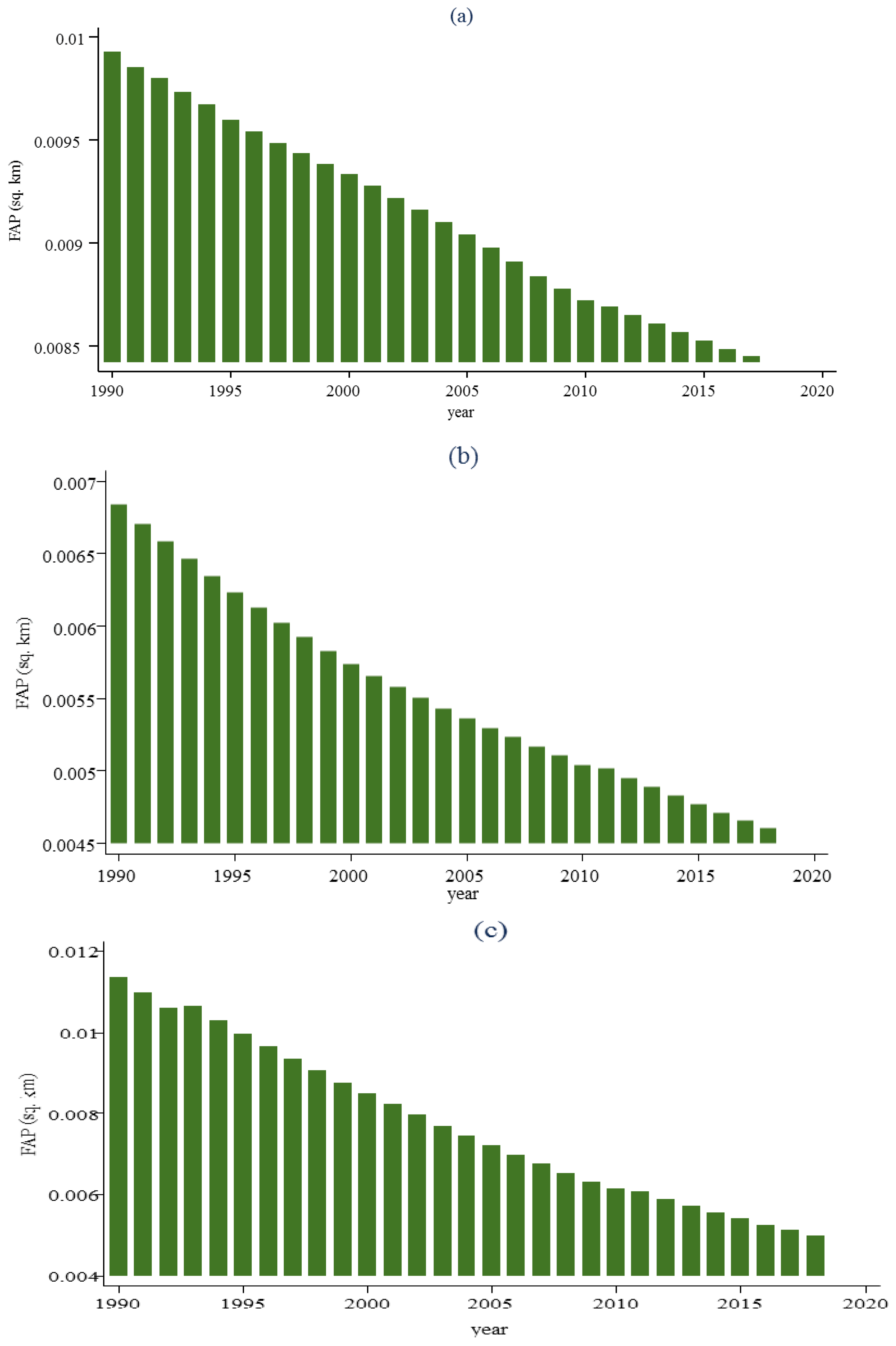
In this context, this research aims to determine the relationship between renewable energy consumption, the gross domestic product (GDP), GDP², non-renewable energy price, population growth and the forest area in three groups of countries during the period 1990–2018. Annual aggregated data are used at the level of three large groups of countries: High-income countries (HIC), middle-income countries (MIC) and low-income countries (LIC), to make a comparison of the factors that determine the forest area. Thus, the dependent variable is represented by per capita forest area measured in square kilometres. As explanatory variables, the following are used: renewable energy consumption and it is measured as the percentage of total energy consumption, GDP at constant 2010 prices, the square of the Gross Domestic Product (GDP²), the non-renewable energy price, measured as the price of a barrel of oil at constant 2018 prices and annual population growth (%). The study supports the hypotheses raised in Section 2.

The structure of this work is as follows. Section 2 describes the literature review, and Section 3 describes the data and the econometric strategy used. In Section 4, the results and discussion of the research are presented. Finally, the conclusions of the research are discussed in Section 5. See Appendix A

Table A1. Abbreviation.

Abbreviation	Description
AIC	Akaike information criteria
ARDL	Autoregressive distributed lag
CDM	Clean development mechanism
CGM	General circulation models
CO2	Carbon dioxide
CUSUM	Cumulative sum
CUSUMQ	Cumulative sum of squares
ECT	Error correction term
EP	Non-renewable energy price
FAO	Food and Agriculture Organisation of the United Nations
FAP	Forest area
FMP	Forest management plan
GDP	Gross domestic product
GDP2	Square of the gross domestic product
GNI	Gross national income
H1	Hypothesis 1
H2	Hypothesis 2
H3	Hypothesis 3
HIC	High-income countries
LIC	Low-income countries
LU	Lower bound
MIC	Middle-income countries
POP	Population growth
REC	Renewable energy consumption
REDD	Reduce deforestation and forest degradation
UB	Upper bound
UNDP	United Nations Development Programme
UNEP	United Nations Environment Programme
WEF	World Economic Forum

.

2. Literature Review

Preserving forest area or reducing deforestation is a global concern, due to the constant demand for forest services [14] and the increasing rates of environmental degradation. In some countries, governments established incentives to avoid deforestation, given that there is competition for the use of forest area [15]. However, in others, the measures taken were incipient. In this regard, deforestation was widely studied to learn more about its determinants and to be able to design measures to mitigate its spread. Over the last few years, various studies have been carried out on the subject, evidencing a long-term relationship between deforestation and energy consumption [12]. Molion [10] is one of the pioneers in relating deforestation with energy consumption, mentioning that renewable energy can reduce CO₂ emissions from greenhouse gases, caused by energy from the consumption of fossil fuels. Another of the highly cited authors who examine the same relationship, deforestation and energy consumption, is Lettau et al. [11], who use the hydrological cycle and atmospheric recycling to study deforestation. These authors indicate that the construction of dams, urbanisation, an increase in the capacity of the irrigation system, increasing energy demands and unsustainable economic growth are determinants of a decrease in the forest area. In this regard, several studies have examined the factors that cause deforestation, and this study focuses on the consumption of renewable energy, economic growth and the non-renewable energy price as determinants of forest area. Thus, there is evidence that argues that deforestation shows a long-term equilibrium relationship with its determinants [12], for which the following hypothesis is established:

Hypothesis 1. (H1)

There is a long-term equilibrium relationship between forest area, GDP, renewable energy consumption and the price of non-renewable energy.

Therefore, the empirical evidence is divided into three groups. The first group includes those studies that examine the effect of renewable energy consumption on deforestation, their contributions being very significant. Thus, Tanner and Johnston [13] found that the government can reduce deforestation rates by applying an ecological policy that expands access to renewable energy to the rural population, so that the consumption of biomass is left for their daily needs. Nazir et al. [16] study the development of the wind energy atlas as a proposal for a partial solution to the problem, which made it possible to confirm a strong relationship between the use of clean energy and deforestation. On the contrary, in Northern Europe, Enevoldsen [17] highlights that the development of wind projects in forest areas has a negative effect on deforestation, which is carried out by installing wind turbines to achieve performance enhancement of renewable energy and reduce the cost of energy, which allows access at a low cost and to give up the consumption of polluting energy.

Brazil, launched the Clean Development Mechanism (CDM), taking into account that 60% of its energy comes from sustainable energy sources. Following this line, Moutinho et al. [18] conduct research, where they show that deforestation rates are related to the energy crisis caused by drought. Stigka et al. [19] confirm the need to replace fossil fuels with clean or renewable energies when producing electricity.

In the same vein, in China, Bhattacharyya and Ohiare [20] found a very close long-term relationship between access to electricity and deforestation. This fact leads them to conclude that ensuring access to electricity to the rural population by the State will help reduce deforestation rates significantly. In the north of Angola, Temudo, Cabral, Talhinhas [21], by using interviews with the heads of households with the observation of the change in vegetation cover, found that deforestation in rural Zaire is comparatively small. Taking into account that the use of biomass for the population’s basic needs has been reduced, the government has intervened by boosting the production of renewable energy.

On the Asian continent, Ahmed et al. [12] conducted a study in Pakistan, the fifth most populated country in the world. By using time series data from 1980–2013, these authors find the existence of cointegration, both in the short and long term, between deforestation and renewable energy consumption. Undoubtedly, this is one of the studies that enables to reinforce the hypothesis raised in this research on the strong links that exist between deforestation, economic growth and energy consumption. For this reason, Houghton and Nassikas [22] recommend that good forest management could stabilise CO2 emissions and would serve to make a successful transition from the use of fossil fuels to the use of energy from renewable resources.

In Colombia, when using General Circulation Models (CGM), Poveda and Mesa [23] mention that a decrease in renewable energy consumption caused by a decrease in river flows leads to an increase in the consumption of forest resources. This in turn, increases deforestation, and consequently, leads to an increase in surface temperature, an increase in atmospheric pressure and mainly a decrease in rainfall in the medium and long term, which generated a decrease in river flows, which in turn, is reflected in severe failures in hydroelectric power systems. The aforementioned circular phenomenon is corroborated by Rojas [24], who confirms that in Colombia, deforestation causes 2.5% of losses in hydroelectric plants. In this sense, the evidence shows that the consumption of renewable energy is positively related to the forest area [13,16], and when there is greater access to clean energy, there is less demand for forest products to use as fuel. Therefore, the following hypothesis of this relationship is proposed:

Hypothesis 2. (H2)

The increase in the consumption of renewable energy is related to the increase in forest cover.

The second group comprises of studies that examine the relationship between the non-renewable energy price and deforestation. For example, in Eisner et al. [25], a positive relationship was found between the rate of global forest loss and the resulting biodiversity loss related to inelastic supplies from oil after 2005. These authors state that while it is true that changes in oil supply and price cause changes in forest cover, this relationship is very challenging, since there are more factors that also influence the change in forest cover, and this is more evident in Southeast Asia and Central America. The authors recommend examining other clean energy options with more elastic prices that do not cause a decrease in forest cover. These recommendations are similar to those made by Scheidel and Sorman [26]. In the same way, studies, such as the one by Abbaspour and Ghazi [27], carry out a pilot model in two rural communities in Iran, Yakhkesh and Pechet, in which the authors find that one of the main reasons for deforestation is an increase in the consumption of fossil fuels as the main source of energy. For this reason, they recommend that this scenario should be considered within the Kyoto protocol, which encourages reducing environmental pollution and deforestation. Furthermore, Czúcz et al. [28] mention that worldwide oil reserves will be depleted, and their price will increase, resulting in consequences for forest conservation, since some non-renewable resources from nature will be used as oil substitutes. Based on the aforementioned, the price of non-renewable energy is a determinant of the forest area [25,27]; consequently, the following hypothesis is proposed:

Hypothesis 3. (H3)

The increase in the price of non-renewable energy is positively related to the decrease in forest cover.

The third group includes all the studies that relate economic growth with deforestation. Research on climate change also generated strong links between economic growth and trade, positioning them as the main drivers of deforestation. This fact has played a great role in the scientific world since the last years of the previous century. In the 1990s, the environmental Kuznets curve was proposed, which establishes the relationship between environmental degradation and economic growth. Since then, some economists, such as Grossman and Krueger [29], Panayotou [30], Selden and Song [31] and Vincent [32], used this hypothesis to verify the existence of an inverted U relationship between economic activity and various forms of environmental degradation. The study by Cropper and Griffiths [33] is one of the pioneers in examining the Kuznets hypothesis, taking into account the relationship between deforestation and economic growth. However, despite the various investigations carried out between deforestation and economic boom, there is no definite consensus on the form that this relationship has [34].

The antecedents presented by the FAO in 1954 and a growing concern about environmental degradation led the academic community to consider deforestation as one of the key indicators of environmental degradation. Some authors, such as Andrée et al. [1], have studied this relationship—finding inverted U-shaped relationships specifically between per capita income and environmental degradation indicators, and concluding that the development and economic growth of a country encourages the consumption of non-renewable resources, which is directly related to deforestation.

It is important to highlight that deforestation is advancing extremely quickly, mainly in South America. However, there is no awareness of the environmental problem generated by economic activity. This is the case of Brazil, which represents most of the worldwide flora and fauna biodiversity, but despite this knowledge, humans and the economy are replacing this biodiversity with commercial land use. By using a linear fixed effects model with a balanced panel of 3168 observations, Santiago and Couto [35] found a long-term relationship between deforestation and the socioeconomic situation between the years 2000 and 2010 in Brazil. The results of this research suggest that investment in agricultural research should be improved to achieve sustainable economic growth and thus, reduce deforestation rates, especially in the Amazon region of Brazil.

In the same country, the authors Arima et al. [14] mention that economic growth continues to advance as investments continue to be made in hydroelectric energy and road paving, which are associated with a high deforestation rate. By 2020, Brazil will have achieved an 80% reduction in deforestation, especially in the Amazon. The authors Carvalho et al. [36] investigated the compensation between environmental conservation and economic growth, using an equilibrium model for 30 Amazonian regions and found that the most affected population would be family farms, but to compensate for this loss, it is estimated that to obtain profits each year, they would have to produce 1.4% of the land. In the same country, Tritsch and Arvor [37] conducted a sub-municipal analysis between socioeconomic development and deforestation in the Brazilian Amazon in their research. Their results confirm a positive relationship between deforestation and economic development, following an environmental Kuznets curve.

In Chile, Apablaza [38] shows the relationship between economic growth and pollution by using linear regressions. In addition, a dummy variable is also used, which identifies the effectiveness of the environmental policies that follow the conceptual behaviour of the Kuznets [39] environmental curve. These results coincide with those by Turner [40]. In Ecuador, Sierra [41] performs a spatial model, where he manages to determine that an increase in economic activity accelerates deforestation growth, reaching very high rates, and in the same way, when growth decreases, deforestation rates also decrease.

Caravaggio [42] studied 114 countries, and found that in high-income and middle-income countries, the boom in economic activity is reflected in the conservation of forest cover. Cuaresma and Heger [43] found that sub-Saharan Africa and low-income group countries have a higher development and deforestation elasticity. Similar results are found in a study carried out by Bhattarai and Hammig [44], whereby using a panel of 66 countries from Asia, Africa and Latin America, quasi-experimental and difference in differences approaches were applied to assess the changes in deforestation produced by economic activity. On the other hand, Tritsch et al. [45] propose that it is mandatory to have a Forest Management Plan (FMP) with logging concessions. The results suggest that applying an FMP will help counteract deforestation significantly, enabling logging companies to carry out extraction cycles to avoid overexploitation. Afawubo and Noglo [46], mention that to reduce deforestation rates, economic development should not be the only focus, but also the institutional quality of countries. This is confirmed by Miyamoto [47], who reveals that poverty has a strong relationship with the change in the forest area. For this reason, it is considered that economic growth generates a greater demand for land [27,36] for other economic and human activities, with which the forest area decreases. Thus, the following hypothesis is established:

Hypothesis 4. (H4)

The increase in economic activity is negatively related to the forest area.

3. Methodology

3.1. Data Sources

This research examines the relationship between renewable energy consumption, GDP, GDP², the non-renewable energy price, population growth and the forest area during the period 1990–2018. The period of examined time has been defined based on the availability of information, especially by the forest cover variable, which has been available in the World Bank [48] since 2018. For this, the aggregate series of countries are used according to their income level: High-income countries (HIC), middle-income countries (MIC) and low-income countries (LIC). Data from the World Bank Development Indicators [48] are used for this study, in which the forest area represents the dependent variable and renewable energy consumption, and the GDP are independent variables. The variable GDP² is included to evaluate the environmental Kuznets curve [39]. The non-renewable energy price is used as an explanatory variable—which refers to the international price of a barrel of oil, which plays an important role in the economic activity, taken from the BP Statistical Review of World Energy [49]. Additionally, population growth is used as an explanatory variable to measure the variation in annual population growth. According to the World Bank [48], the classification of countries is based on Gross National Income (GNI) per capita in United States dollars. HIC have a GNI per capita greater than $12,055, MIC between $996–12,055 and LIC $995 or less.

Appendix A

Table A2. Countries according to income group.

HIC		MIC		LIC
1	Andorra	1	Albania	1	Afghanistan
2	Antigua And Barbuda	2	Algeria	2	Burkina Faso
3	Aruba	3	American Samoa	3	Burundi
4	Australia	4	Angola	4	Central African Republic
5	Austria	5	Argentina	5	Chad
6	Bahamas, The	6	Armenia	6	Congo, Dem. Rep.
7	Bahrain	7	Azerbaijan	7	Eritrea
8	Barbados	8	Bangladesh	8	Ethiopia
9	Belgium	9	Belarus	9	Gambia, The
10	Bermuda	10	Belize	10	Guinea
11	British Virgin Islands	11	Benin	11	Guinea-Bissau
12	Brunei Darussalam	12	Bhutan	12	Haiti
13	Canada	13	Bolivia	13	Korea, Dem. People’s Rep.
14	Cayman Islands	14	Bosnia And Herzegovina	14	Liberia
15	Channel Islands	15	Botswana	15	Madagascar
16	Chile	16	Brazil	16	Malawi
17	Croatia	17	Bulgaria	17	Mali
18	Curacao	18	Cabo Verde	18	Mozambique
19	Cyprus	19	Cambodia	19	Niger
20	Czech Republic	20	Cameroon	20	Rwanda
21	Denmark	21	China	21	Sierra Leone
22	Estonia	22	Colombia	22	Somalia
23	Faroe Islands	23	Comoros	23	South Sudan
24	Finland	24	Congo, Rep.	24	Sudan
25	France	25	Costa Rica	25	Syrian Arab Republic
26	French Polynesia	26	Cote D’ivoire	26	Tajikistan
27	Germany	27	Cuba	27	Togo
28	Gibraltar	28	Djibouti	28	Uganda
29	Greece	29	Dominica	29	Yemen, Rep.
30	Greenland	30	Dominican Republic
31	Guam	31	Ecuador
32	Hong Kong Sar, China	32	Egypt, Arab Rep.
33	Hungary	33	El Salvador
34	Iceland	34	Equatorial Guinea
35	Ireland	35	Eswatini
36	Isle Of Man	36	Fiji
37	Israel	37	Gabon
38	Italy	38	Georgia
39	Japan	39	Ghana
40	Korea, Rep.	40	Grenada
41	Kuwait	41	Guatemala
42	Latvia	42	Guyana
43	Liechtenstein	43	Honduras
44	Lithuania	44	India
45	Luxembourg	45	Indonesia
46	Macao Sar, China	46	Iran, Islamic Rep.
47	Malta	47	Iraq
48	Mauritius	48	Jamaica
49	Monaco	49	Jordan
50	Nauru	50	Kazakhstan
51	Netherlands	51	Kenya
52	New Caledonia	52	Kiribati
53	New Zealand	53	Kosovo
54	Northern Mariana Islands	54	Kyrgyz Republic
55	Norway	55	Lao Pdr
56	Oman	56	Lebanon
57	Palau	57	Lesotho
58	Panama	58	Libya
59	Poland	59	Malaysia
60	Portugal	60	Maldives
61	Puerto Rico	61	Marshall Islands
62	Qatar	62	Mauritania
63	Romania	63	Mexico
64	San Marino	64	Micronesia, Fed. Sts.
65	Saudi Arabia	65	Moldova
66	Seychelles	66	Mongolia
67	Singapore	67	Montenegro
68	Sint Maarten (Dutch Part)	68	Morocco
69	Slovak Republic	69	Myanmar
70	Slovenia	70	Namibia
71	Spain	71	Nepal
72	St. Kitts And Nevis	72	Nicaragua
73	St. Martin (French Part)	73	Nigeria
74	Sweden	74	North Macedonia
75	Switzerland	75	Pakistan
76	Trinidad And Tobago	76	Papua New Guinea
77	Turks And Caicos Islands	77	Paraguay
78	United Arab Emirates	78	Peru
79	United Kingdom	79	Philippines
80	United States	80	Russian Federation
81	Uruguay	81	Samoa
82	Virgin Islands (U.S.)	82	Sao Tome And Principe
		83	Senegal
		84	Serbia
		85	Solomon Islands
		86	South Africa
		87	Sri Lanka
		88	St. Lucia
		89	St. Vincent And The Grenadines
		90	Suriname
		91	Tanzania
		92	Thailand
		93	Timor-Leste
		94	Tonga
		95	Tunisia
		96	Turkey
		97	Turkmenistan
		98	Tuvalu
		99	Ukraine
		100	Uzbekistan
		101	Vanuatu
		102	Venezuela, Rb
		103	Vietnam
		104	West Bank And Gaza
		105	Zambia
		106	Zimbabwe

Source: According to the world bank data [48].

describes the countries examined according to their income level. The description of the variables used in the model is shown in

Table 1. Description of variables used in the study.

Variables	Symbol	Unit of Measurement	Data Sources
Forest area	FAP	Square kilometres per capita	World Bank [50]
Renewable energy consumption	REC	Log % of total final energy consumption	World Bank [50]
Gross domestic product	GDP	Log US $ constant 2010 prices per capita	World Bank [50]
Square of the Gross domestic product	GDP2	Log of the square of GDP per capita	World Bank [50]
Non-renewable energy price	EP	Log US $ constant prices of 2018	BP Statistical Review of World Energy [51]
Population growth	POP	Percentage of annual population growth (%)	World Bank [50]

. All the variables are expressed in their logarithmic form to reduce their measurement scale, with the exception of the dependent variable, which has relatively low values and population growth.

The descriptive statistics and the correlation matrix are shown in

Table 2. Descriptive statistics and correlation matrix.

Groups	Variable	Observations	Mean	Std. Dev.	Min	Max	Correlation
HIC	FAP	29	0.0091	0.0004	0.0084	0.0099	-
	REC	29	2.1055	0.2203	1.8609	2.5194	−0.9388 *
	GDP	29	10.4993	0.1256	10.2798	10.6823	−0.9789 *
	GDP2	29	20.99866	0.2512614	20.5597	21.36461	−0.9789 *
	EP	29	3.9444	0.5393	2.9749	4.8218	−0.7365 *
	POP	29	0.6470451	0.0998829	0.447717	0.8397276	0.5938 *
MIC	FAP	29	0.0055396	0.0006618	0.0046022	0.0068432	-
	REC	29	3.411611	0.1040366	3.245336	3.538147	0.8779 *
	GDP	29	8.037406	0.334049	7.630042	8.594371	−0.9541 *
	GDP2	29	16.07481	0.6680981	15.26008	17.18874	−0.9541 *
	EP	29	3.944403	0.5393446	2.974963	4.82188	−0.7006 *
	POP	29	1.346662	0.2254831	1.077227	1.907097	0.9741
LIC	FAP	29	0.0077	0.0019	0.0049	0.0113	-
	REC	29	4.2846	0.0570	4.1402	4.3919	−0.8462 *
	GDP	29	6.3448	0.1530	6.1508	6.6151	−0.8717 *
	GDP2	29	12.6896	0.3061791	12.30172	13.23003	−0.8717 *
	EP	29	3.9444	0.5393	2.9749	4.8218	−0.7334 *
	POP	29	2.768654	0.1385192	2.543851	2.993388	0.7579 *

Note: * indicates significance level at 5%. HIC, high-income countries; MIC, middle-income countries; LIC, low-income countries.

. At 5% significance, it can be seen that there is a strong negative relationship between renewable energy consumption, the GDP, GDP², the non-renewable energy price and the forest area, except for MIC countries in which a positive relationship between REC and FAP is seen. In addition, POP shows a positive and significant relationship with the forest area.

Figure 1 shows the annual evolution of per capita forest area measured in square kilometres for each of the groups of countries. In addition, it is observed that in 2018 the per capita forest area in HIC is approximately double of that in MIC and LIC.

3.2. Econometric Model

The main objective of this document is to find the relationship between renewable energy consumption, the GDP, GDP², the non-renewable energy price, population growth and the forest area in different groups of countries classified according to their income level. Thus, the model specification can be written as:

$$FA{P}_t={\beta }_0+{\beta }_{1}RE{C}_t+{\beta }_{2}GD{P}_t+{\beta }_{3}GD{P}_t^2+{\beta }_{4}E{P}_t+{\beta }_{5}PO{P}_t+{\epsilon }_t$$

(1)

In Equation (1), $FA{P}_t$ represents the forest area at time $t=1990, 1991, 1992,\dots 2018$; $RE{C}_t$ represents renewable energy consumption; $GD{P}_t$ is the domestic product; $GD{P}_t^2$ is the square of GDP; $E{P}_t$ is the price of non-renewable energy; $PO{P}_t$ represents population growth; ${\beta }_i$ denotes the coefficients of the explanatory variables and ${\epsilon }_t$ is the error term.

Next, various econometric strategies are applied, according to what is described in the following sections.

3.2.1. Stationary Tests

To fulfil the objective of the study, the stationarity of the series must be examined. One of the most widely used formal methods to assess stationarity is the Augmented Dickey-Fuller [50] unit root test. The null hypothesis $\left({\mathrm{H}}_0:\mathsf{\rho }=0\right)$ assumes that the variable contains a unit root, while the alternative hypothesis $\left({\mathrm{H}}_1:\mathsf{\rho }=1\right)$ states that it does not contain a unit root. To examine the long-term relationship, the variables examined may have a different order of integration, I (0), I (1) or a mixture of the two, so the ARDL approach becomes suitable for performing the cointegration analysis [51,52,53]. However, a limitation of the ARDL approach is that it cannot be used with variables with integration order I (2), the maximum order is I (1). In addition, the unit root test of Kwiatkowski is performed [54]. Equation (2) formalises this relationship, where $t$ represents the year and $i$ the number of lags of the variable:

$$∆{\mathrm{y}}_{\mathrm{t}}=\mathrm{c}+{\mathsf{\rho }\mathrm{y}}_{\mathrm{t}-1}+{\displaystyle \sum }_{\mathrm{i}=1}^{\mathrm{p}}{\varnothing }_{\mathrm{i}}∆{\mathrm{y}}_{\mathrm{t}-\left(\mathrm{i}-1\right)}+{\mathsf{\epsilon }}_{\mathrm{t}}$$

(2)

3.2.2. Cointegration Method

The time series cointegration method is used to examine the long-term relationship between the variables. Consequently, Pesaran, Shin and Smith [55] are followed to apply the Autoregressive Distributed Lag (ARDL) Model, since it analyses the cointegration between variables with different degrees of cointegration, and also controls endogeneity [7,56] and allows use for short periods—even with observations less than 30 [57,58]. An indispensable requirement is that the stationarity order must be at most I (1), otherwise the analysis is invalid [59,60,61,62]. The relationship is formalised in the following equation:

$$\begin{array}{l}∆FA{P}_t={\alpha }_1+{\alpha }_{2}FA{P}_{t-1}+{\alpha }_{3}RE{C}_{t-1}+{\alpha }_{4}GD{P}_{t-1}+{\alpha }_{5}GD{P}_{t-1}^2+{\alpha }_{5}E{P}_{t-1}\\ +{\alpha }_{6}PO{P}_{t-1}+{\displaystyle {\displaystyle \sum }_{k=1}^n}{\beta }_{1k}FA{P}_{t-k}+{\displaystyle {\displaystyle \sum }_{k=1}^n}{\beta }_{2k}RE{C}_{t-k}\\ +{\displaystyle {\displaystyle \sum }_{k=1}^n}{\beta }_{3k}GD{P}_{t-k}+{\displaystyle {\displaystyle \sum }_{k=1}^n}{\beta }_{4k}GD{P}_{t-k}^2+{\displaystyle {\displaystyle \sum }_{k=1}^n}{\beta }_{5k}E{P}_{t-k}\\ +{\displaystyle {\displaystyle \sum }_{k=1}^n}{\beta }_{6k}PO{P}_{t-k}+{\epsilon }_t\end{array}$$

(3)

In Equation (3), $∆$ is the difference operator. ${\alpha }_1$ is the constant term, ${\alpha }_2,{\alpha }_3,{\alpha }_4,{\alpha }_5$ are the long-term coefficients. ${\beta }_1,{\beta }_2,{\beta }_3,{\beta }_4, {\beta }_5, {\beta }_6$ represent error correction dynamics. ${\epsilon }_t$ is the error term $k$ represents the number of lags for each variable. The ARDL model uses the Wald test (F-Statistic) to determine long-term existence. The null hypothesis establishes no cointegration between the variables $\left(H_0:{\beta }_1={\beta }_2={\beta }_3={\beta }_4={\beta }_5={\beta }_6=0\right)$ against the alternative hypothesis that establishes cointegration between the variables $\left(H_0:{\beta }_1\ne {\beta }_2\ne {\beta }_3\ne {\beta }_4\ne {\beta }_5\ne {\beta }_6\ne 0\right)$. In the cointegration analysis, Pesaran, Shin and Smith [55] establish the critical values of F-statistics and two types of limits: Lower and upper. If F-statistics is less than the lower limit, the null hypothesis of no cointegration is accepted. In contrast, if F-statistics is greater than the upper limit, the null hypothesis is rejected—that is, there is long-term cointegration between the variables. In the case that the value is between the lower and upper limit, the results are inconclusive. Finally, the Akaike [63] criterion is used to determine the optimal lag of the variables.

3.2.3. Error Correction Term

Once long-term cointegration has been verified, Error Correction Term (ECT) is examined. The model specification is described below:

$$\begin{array}{l}∆FA{P}_t={\beta }_0+{\displaystyle {\displaystyle \sum }_{k=1}^n}{\beta }_{1k}∆FA{P}_{t-k}+{\displaystyle {\displaystyle \sum }_{k=1}^n}{\beta }_{2k}∆RE{C}_{t-k}+{\displaystyle {\displaystyle \sum }_{k=1}^n}{\beta }_{3k}∆GD{P}_{t-k}\\ +{\displaystyle {\displaystyle \sum }_{k=1}^n}{\beta }_{4k}∆GD{P}_{t-k}^2+{\displaystyle {\displaystyle \sum }_{k=1}^n}{\beta }_{5k}∆E{P}_{t-k}+{\displaystyle {\displaystyle \sum }_{k=1}^n}{\beta }_{6k}∆PO{P}_{t-k}\\ +\gamma EC{T}_{t-1}+{\epsilon }_t\end{array}$$

(4)

In Equation (4), $EC{T}_{t-1}$ represents the calculated error term of the cointegration equation that reflects the non-equilibrium error that deviates from the long-term equilibrium relationship.$\gamma$ describes the adjustment parameters and the speed at which the variables return to the long-term equilibrium relationship.

Finally, the stability of the model is checked using the diagnostic test, which checks if the model is free of serial autocorrelation and heteroscedasticity. Likewise, the correct specification, normality (JB) and stability are verified, using the Ramsey, Jarque-Bera and the cumulative sum of squares of recursive residuals proposed by Brown et al. [64], respectively. Figure 2 summarises the methodology used in this investigation.

4. Discussion of Results

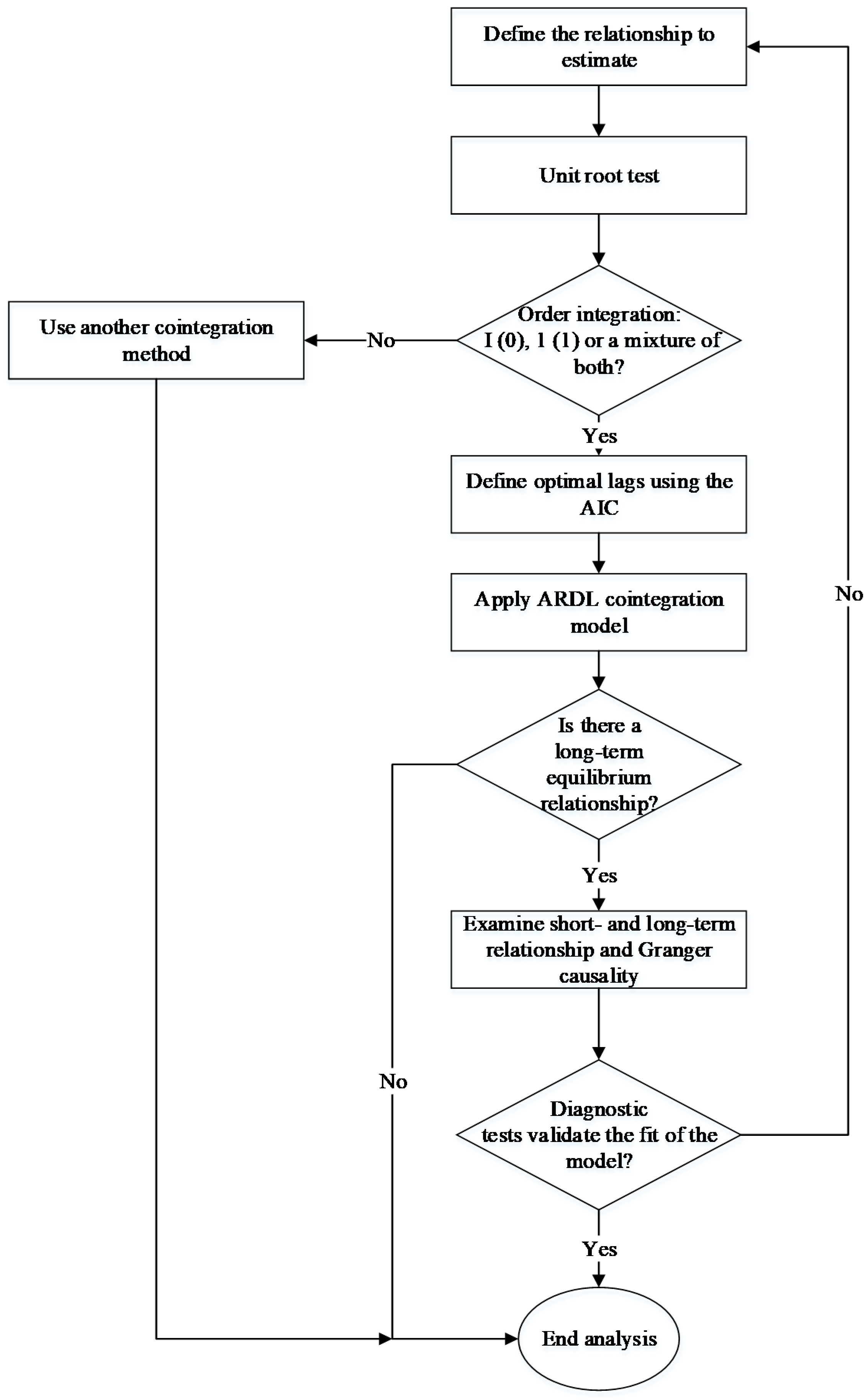
Prior to the long-term analysis, the stationarity of the variables was examined by using the Augmented Dickey-Fuller unit root test (ADF) [50]. The results of

Table 3. Unit root test.

Groups	HIC				MIC				LIC
	ADF		KPSS		ADF		KPSS		ADF		KPSS
	WT	WOT	WT	WOT	WT	WOT	WT	WOT	WT	WOT	WT	WOT
Levels
FAP	−4.481 ***	−5.23 ***	0.473 ***	0.45 ***	−15.253 ***	−18.11 ***	0.685 ***	0.34 ***	−3.758 ***	−4.52 ***	0.686 ***	0.67 ***
GDP	−1.171	−1.45	0.594 ***	0.64 ***	2.309	1.32	0.533 ***	0.67 ***	1.658	1.56	0.528 ***	0.45 ***
GDP2	−1.171	−1.45	0.594 ***	0.64 ***	2.309	1.32	0.533 ***	0.67 ***	1.658	1.56	0.528 ***	0.45 ***
REC	−3.617 **	−5.23 ***	0.665 ***	0.67 ***	1.297	1.67	0.481 ***	0.56 ***	−1.991	−1.867	0.305 ***	0.75 ***
EP	−1.176	−1.53	0.284 ***	0.56 ***	−1.176	−1.53	0.284 ***	0.56 ***	−1.176	−1.53	0.284 ***	0.56 ***
POP	−6.23 ***	−8.24 ***	0.647 ***	0.23 ***	−7.23 ***	−8.23 ***	0.23 ***	0.36 ***	−6.81 ***	−7.19 ***	0.56 ***	0.76 ***
First difference
FAP	−1.864	−3.345 ***	0.259 ***	0.34 ***	−1.952	−2.72 **	0.419 ***	0.56 ***	−4.280 ***	−3.56 ***	0.435 ***	0.72 ***
GDP	−4.021 ***	−5.67 ***	0.562 ***	0.45 ***	−2.873 **	−3.45 ***	0.364 ***	0.12 **	−2.941 *	−6.24 ***	0.371 ***	0.45 ***
GDP2	−4.021 ***	−5.67 ***	0.562 ***	0.45 ***	−2.873 **	−3.45 ***	0.364 ***	0.12 **	−2.941 *	−6.24 ***	0.371 ***	0.45 ***
REC	−3.780 ***	−5.93 ***	0.456 ***	0.35 ***	−2.715 **	−4.67 ***	0.372 ***	0.37 ***	−4.305 ***	−7.56 ***	0.303 ***	0.34 ***
EP	−4.372 ***	−5.67 ***	0.118 *	0.45 ***	−4.372 ***	−5.67 ***	0.118 *	0.45 ***	−4.372 ***	−5.67 ***	0.118 *	0.45 ***
POP	−7.23 ***	−7.35 ***	0.46 ***	0.45 ***	−6.78 ***	−8.34 ***	0.67 ***	0.56 ***	−9.61 ***	−9.89 ***	0.23 ***	0.67 ***

Note: ***, **, * indicates the significance level at 1%, 5% and 10%, respectively. WT = with trend and WOT = Without trend.

rejects the null hypothesis that assumes the existence of a unit root—that is, the series are stationary. One of the main advantages is that the ARDL approach can use variables with integration order I (0), I (1) or a mixture of both [65]. Complementarily, it is carried out on Kwiatkowski, Phillips, Schmidt and Shin (KPSS) [54]. Thus, the forest area and population growth variable for all groups is stationary at levels I (0) and the rest of the independent variables at I (1).

After checking the stationarity of the series,

Table 4. ARDL cointegration test.

Group	F	Optimal Lags	F–Statistics
			10%		5%		1%
			LB	UB	LB	UB	LB	UB
HIC	1.445	(2 2 2 3 2 1)	2.45	3.52	2.86	4.01	3.74	5.06
MIC	18.57 ***	(1 2 2 1 1 1)	2.45	3.52	2.86	4.01	3.74	5.06
LIC	12.037 ***	(2 2 1 2 1 1)	2.45	3.52	2.86	4.01	3.74	5.06

Note: *** indicates the 1% level of significance. The values in parenthesis indicate the optimal lag of each variable (FAP, GDP, GDP2, REC, EP, POP). LB = Lower bound. UB = Upper bound.

presents the results of the ARDL cointegration test. To properly determine the optimal lag length of each variable, the Akaike information criteria (AIC) is used. In MIC and LIC, the calculated F–statistics are higher than the value of the upper limit proposed by Pesaran, Shin and Smith [55]. Consequently, at the 1% significance level, the alternative hypothesis that establishes a long-term cointegration relationship between the study variables is accepted, which means that the variables move jointly over time. On the contrary, for HIC, the results show no equilibrium relationship in the model studied.

The findings of the cointegration test evaluate the long-term relationship between the forest area, GDP, GDP², renewable energy consumption, non-renewable energy price and population growth. Thus, the ARDL approach is used to estimate the long-term coefficients between the variables.

Table 5. Long–run estimations.

	HIC		MIC		LIC
Dependent Variable: FAP	Coefficient	p-Value	Coefficient	p-Value	Coefficient	p-Value
${\mathrm{FAP}}_{\mathrm{t}-1}$	0.0014501	0.473	−0.0044839 ***	0.0015	−0.0876817 ***	0.000
REC	−0.0452131	0.356	0.041512 **	0.047	0.027512 *	0.081
GDP	0.0130313	0.745	−0.0623161 *	0.063	−0.0532092 ***	0.004
GDP2	0.0000328	0.263	0.0000238	0.362	0.0000048	0.762
EP	0.0002703	0.924	0.0011696	0.841	0.0011509	0.197
POP	0.0088715	0.603	−0.0234771 **	0.035	−0.0024849 *	0.085

Note: ***, **, * indicates the significance level at 1%, 5% and 10%, respectively.

shows the results obtained, ${\mathrm{FAP}}_{\mathrm{t}-1}$ represents the error correction term (ECT), in MIC and LIC is negative and statistically significant as expected. However, in the HIC, its value is positive and not significant, which shows the long-term non-cointegration mentioned above. The values of ${\mathrm{FAP}}_{\mathrm{t}-1}$ range from 0 (no adjustment) to −1 (immediate adjustment) as expected. Its values are small, which is reasonable, since increasing forest cover is a time-consuming process inherent in its nature. That is, when the forest cover area is far from its equilibrium level, it is adjusted by 0.44% and 8.7%, respectively, within the first year. The speed of reaching the equilibrium level is slow and significant. In MIC and LIC, an increase of 1% in renewable energy consumption represents an increase of 0.041512 km2 and 0.027512 km2 of forest area, respectively. That is, energy consumption from renewable sources contributes to reducing deforestation. The increase in the consumption of renewable energy represents an alternative for access to clean energy, instead of wood from forests, which is used as energy sources. These results are consistent with those reported by Tanner and Johnston [13], Nazir et al. [16] and Bhattacharyya and Ohiare [20], who affirm that the State can generate policies so that the rural population can have access to electricity and give up the consumption of products from forests.

Regarding an increase in economic activity in MIC and LIC, measured by GDP, it decreases the forest area. The increase in economic activity brings with it some externalities, such as increased urbanisation, expansion of crops to provide food, among others, which generally is related to a greater demand for land and to achieve this, spaces that are destined for forests are occupied. These findings are also based on the fact that the increase in economic activity demands resources that are found in the forests, which leads to a process of deforestation [43,66].

On the other hand, population growth is negatively related to forest area coverage in both groups of countries (Table 5). That is, as the population increases, a change in land use is generated in which the forest area is used for another type of human activity, such as growing food, spaces for housing, resources (wood) for the construction of houses, among others. These results coincide with those found by Ahmed, Shahbaz, Qasim and Long [12], who mention that the increase in the population density demands more forest resources for the construction of housing in the rural sector. Moreover, Tritsch and Le Tourneau [67] find that one third of deforestation in the Amazon region of Brazil is associated with 1.5% of the population. The findings described in this section provide sufficient information to verify the fulfilment of hypotheses H1, H2 and H4 raised in Section 2. Additionally, it is observed that the price of non-renewable energy is not significant, thus ruling out hypothesis H3. Similarly, GDP² is not significant—that is, non-compliance with the environmental Kuznets curve is corroborated [39].

Following the long-term analysis, the short-term test between the model variables is evaluated.

Table 6. Short–run estimations.

	HIC		MIC		LIC
Dependent Variable: FAP	Coefficient	p-Value	Coefficient	p-Value	Coefficient	p-Value
REC	−0.0000154	0.325	0.0000447	0.833	−0.0023418	0.141
GDP	0.0000431	0.217	−0.0002613	0.542	0.0010047	0.431
EP	9.88 × 10−7	0.630	−8.40 × 10−7	0.924	−0.0000574	0.251
POP	−0.000094	0.488	0.0002623	0.942	−0.0006314	0.599

shows that the variation in renewable energy consumption, GDP, GDP², the non-renewable energy price, population growth are not related to the immediate changes in the forest area in the short term in all three models.

Subsequently, the error-correction term (ECT) of the Granger causality test is used to detect the direction of long-term causality between the study variables.

Table 7. ECT Granger causality.

Direction of Granger Causality	Long-Run
	${\mathbf{ECT}}_{\mathbf{t}-1}$
REC, GDP, GDP2, EP, POP $\to$ FAP	HIC	0.0014501
	MIC	−0.0044839 ***
	LIC	−0.0876817 ***

Note: *** indicates the significance level at 1%.

shows that in the long term, renewable energy consumption, GDP, GDP², the non-renewable energy price and population growth causes the forest area in MIC and LIC.

Additionally,

Table 8. ARDL model long-run diagnostic test.

Diagnostic Test	HIC	MIC	LIC
	p-Value	p-Value	p-Value
Model Specified	0.3456	0.4944	0.4982
Serial correlation	0.2678	0.4043	0.3256
Heteroscedasticity	0.4576	0.4076	0.5835
Normality	0.8204	0.5734	0.7683
R2	77.45	83.87	84.89

shows the diagnostic tests to validate the model fit [12,52,53,56] for all groups of countries. The p-value greater than 0.05 of the Ramsey test confirms that the models are correctly specified. The p-value greater than 0.05 rules out the presence of serial correlation in the estimated models. The p-value of the heteroscedasticity test, which is greater than 0.05, confirms that the models are homoscedastic. Moreover, the Jarque-Bera normality test with a probability of 0.8204, 0.5734 and 0.7683, confirms that the residuals are normally distributed. Finally, the coefficient of determination of 77.45, 83.87 and 84.89, respectively, indicate the good fit of the model.

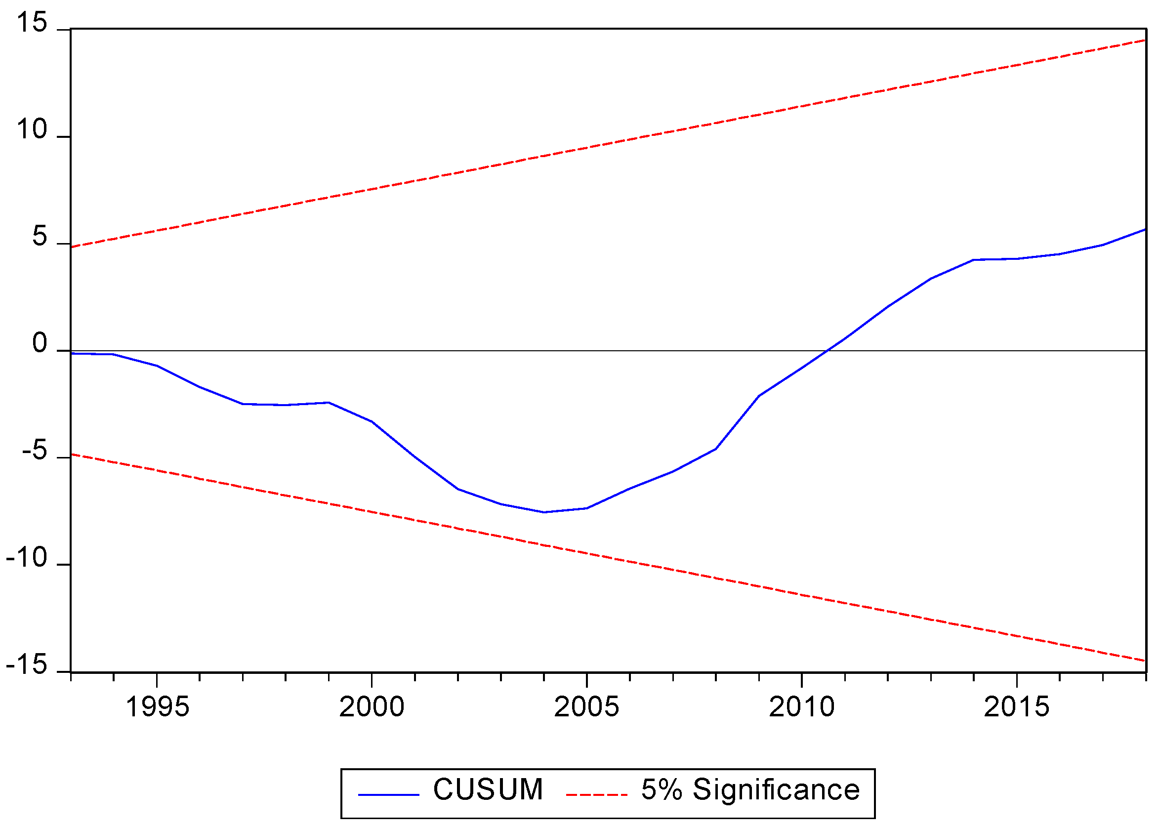
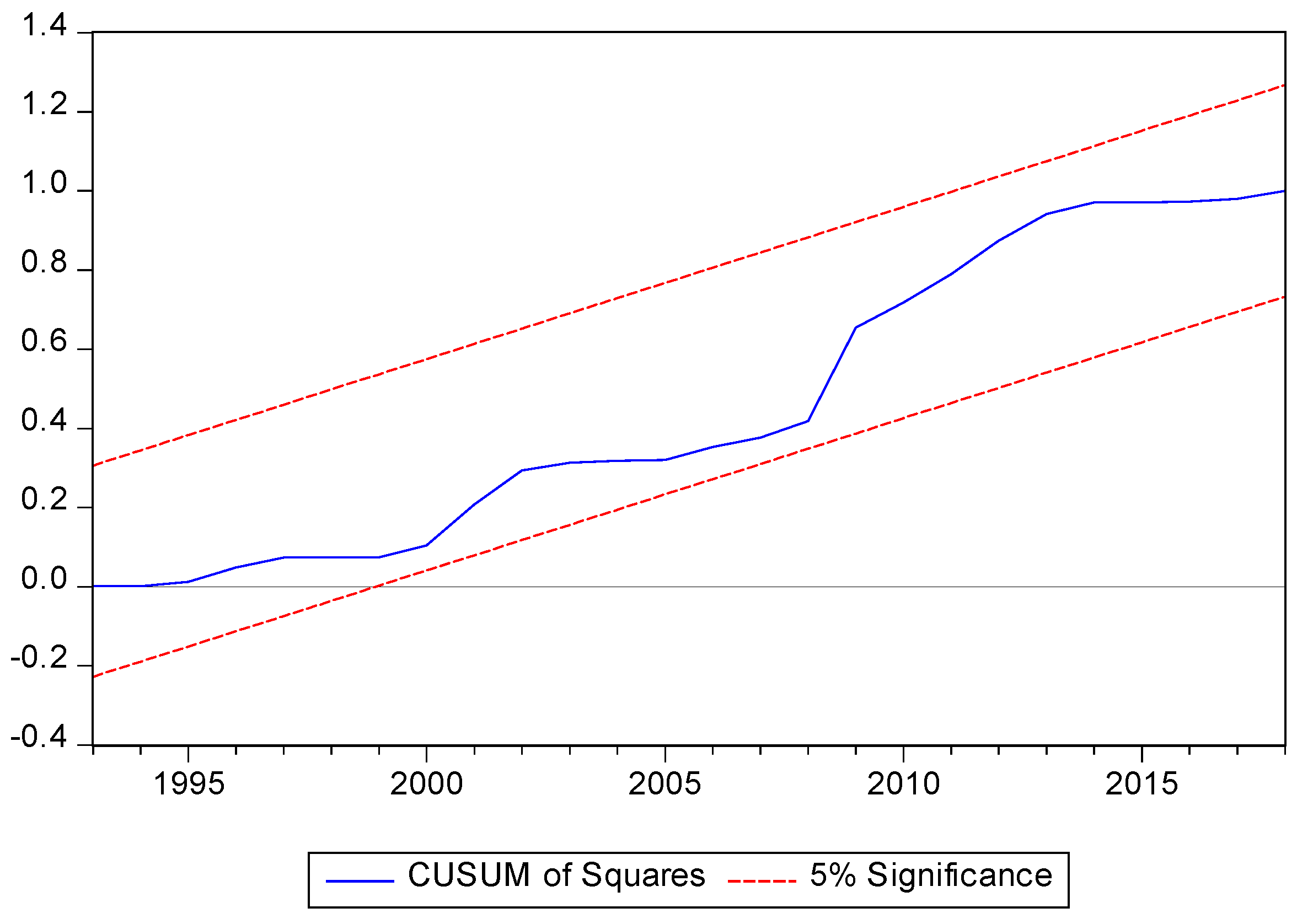
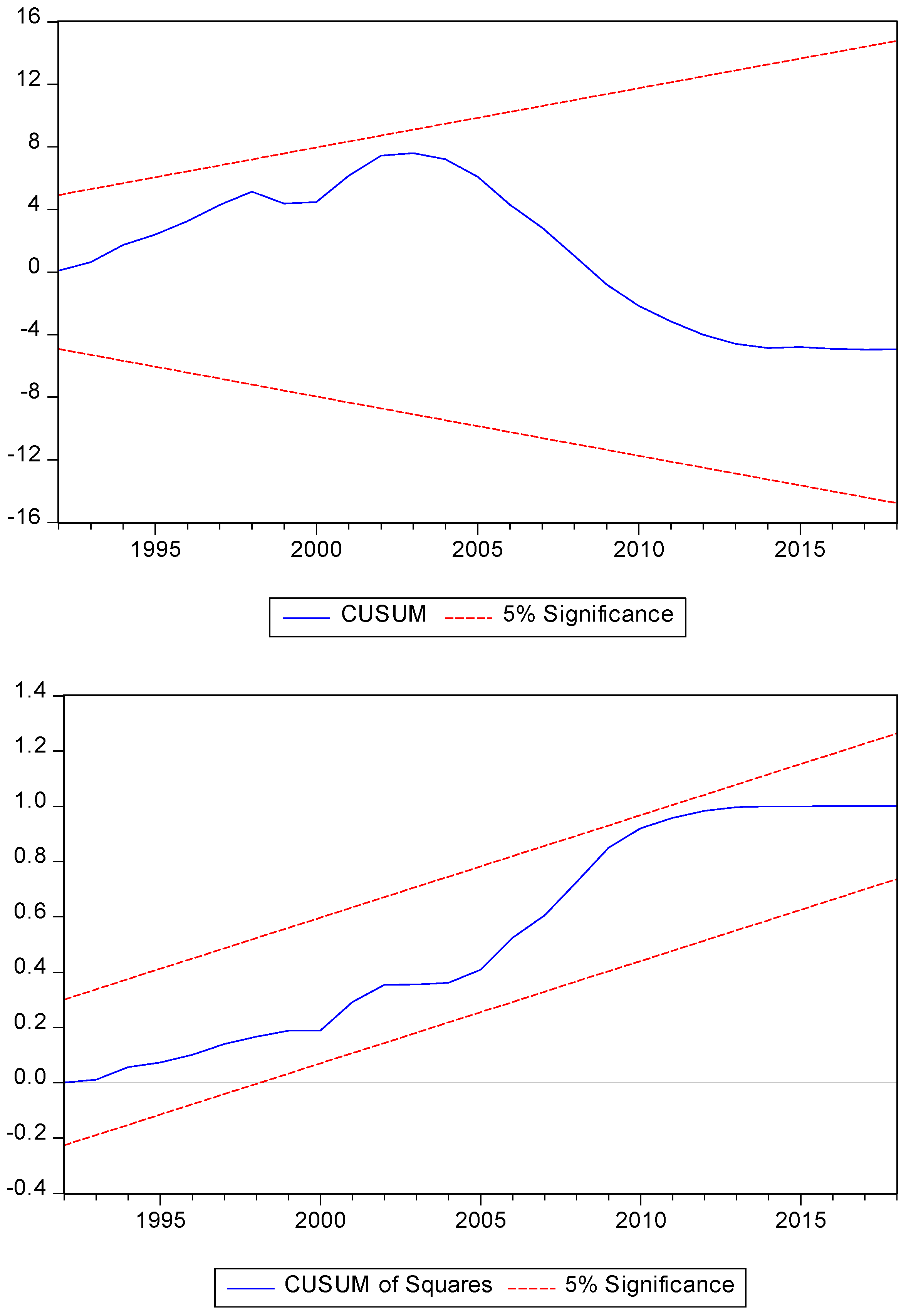
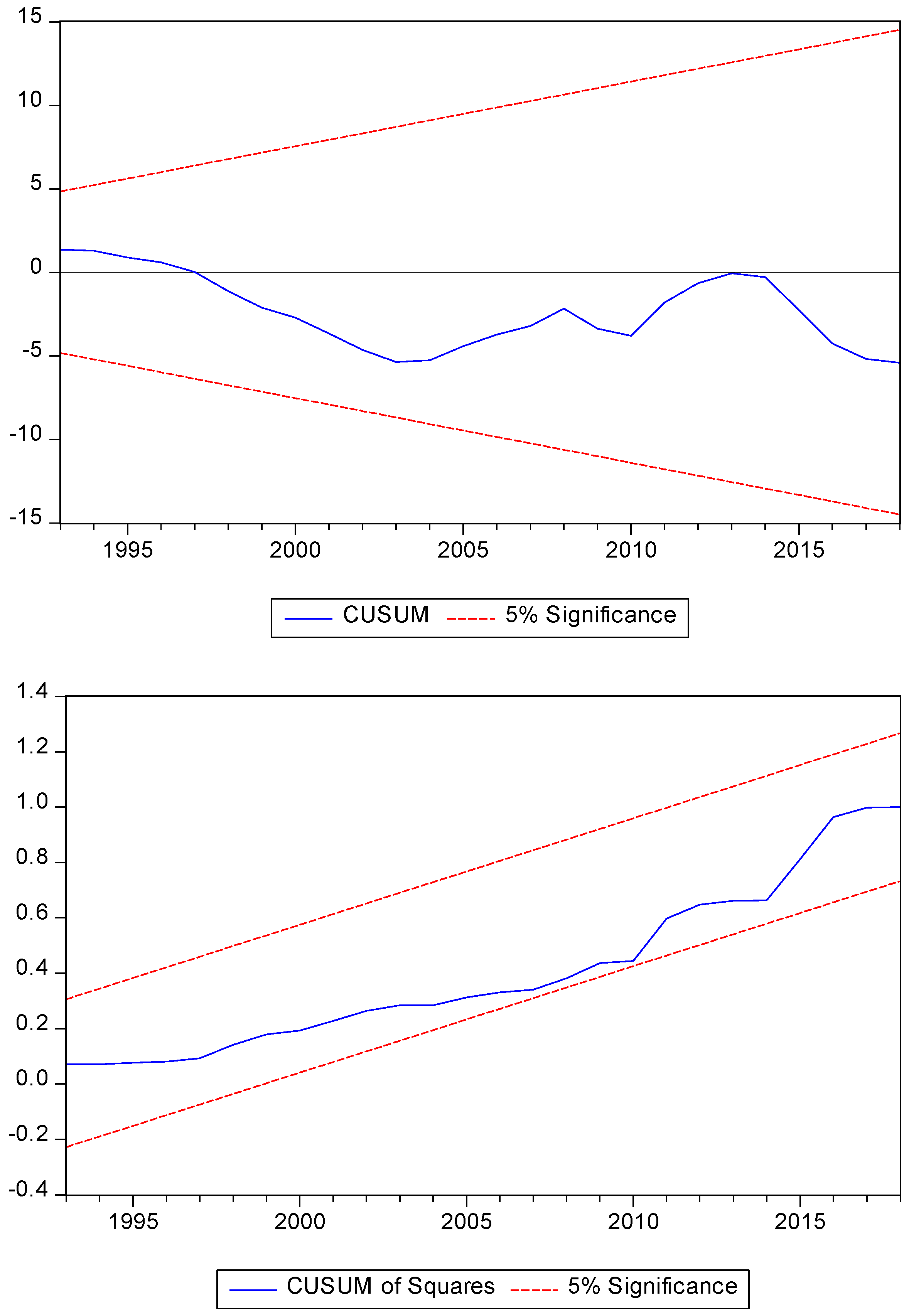
To conclude the study, following Brown et al. [64], the stability of the parameters is evaluated. The cumulative sum (CUSUM) and cumulative sum of squares (CUSUMQ) are observed in Figure 3, Figure 4 and Figure 5 for all groups of countries. In all three models, the graph shows that the lines are at the critical limit of 95%, which indicates the stability of the coefficients. Diagnostic tests confirm that the ARDL model is reliable for defining policies at the linking point of forest area, renewable energy consumption, GDP, GDP², non-renewable energy price and population growth.

5. Conclusions and Policy Implications

Deforestation is a global economic and environmental problem, so trying to understand its determinants is essential to mitigate its accelerated pace. This research examined the long-term equilibrium relationship between renewable energy consumption, GDP, GDP², renewable energy price, population growth and forest area in high-, middle- and low-income countries, using the ARDL econometric approach.

The results confirm a long-term equilibrium relationship between the mentioned variables for MIC and LIC. The ECT indicates that the speed of forest cover adjustment is slow when it is not at its equilibrium point, approximately it adjusts by 0.44% and 8.7%, respectively, within the first year. Furthermore, the consumption of renewable energy is positively related to the forest area. In contrast, population growth maintains a negative relationship with the forest area. The results obtained provide valuable information to confirm the fulfilment of the hypotheses of this investigation, H1, H2 and H4. On the contrary, the H4 is not fulfilled.

Those responsible for establishing public and environmental policy measures must consider that encouraging the consumption of renewable energy allows for an alternative to the use of forest products and services. In MIC and LIC, the boom in economic activity must take place in scenarios in which environmental sustainability and the care of forests are on the horizon. Population growth must be associated with sustainable measures on land use, thereby ensuring that deforestation does not increase.

One of the main limitations of this research is the lack of information on the price elasticity of demand for agricultural products throughout the period analysed, to include them as an explanatory variable and evaluate how it is correlated with deforestation. Likewise, the period of time examined is a function of the availability of the information.

References

1. Andrée, B.P.J.; Chamorro, A.; Spencer, P.; Koomen, E.; Dogo, H. Revisiting the relation between economic growth and the environment; a global assessment of deforestation, pollution and carbon emission. Renew. Sustain. Energy Rev. 2019, 114, 109–221. [Google Scholar] [CrossRef]
2. Mäntymaa, E.; Tyrväinen, L.; Juutinen, A.; Kurttila, M. Importance of forest landscape quality for companies operating in nature tourism areas. Land Use Policy 2019, 104095. [Google Scholar] [CrossRef]
3. WEF. World Economic Forum: Cologny/Geneva Switzerland. 2020. Available online: https://www.weforum.org/ (accessed on 21 June 2020).
4. FAO. Organización de las Naciones Unidad para la Alimentación y la Agricultura. 2019. Available online: http://www.fao.org/home/es/ (accessed on 21 June 2020).
5. Suwal, N.; Huang, X.; Kuriqi, A.; Chen, Y.; Pandey, K.P.; Bhattarai, K.P. Optimisation of cascade reservoir operation considering environmental flows for different environmental management classes. Renew. Energy 2020, 158, 453–464. [Google Scholar] [CrossRef]
6. Kuriqi, A.; Pinheiro, A.N.; Sordo-Ward, A.; Garrote, L. Water-energy-ecosystem nexus: Balancing competing interests at a run-of-river hydropower plant coupling a hydrologic–ecohydraulic approach. Energy Convers. Manag. 2020, 223, 113267. [Google Scholar] [CrossRef]
7. Khan, S.A.R.; Yu, Z.; Belhadi, A.; Mardani, A. Investigating the effects of renewable energy on international trade and environmental quality. J. Environ. Manag. 2020, 272, 111089. [Google Scholar] [CrossRef]
8. Khan, S.A.R.; Yu, Z.; Sharif, A.; Golpîra, H. Determinants of economic growth and environmental sustainability in South Asian Association for Regional Cooperation: Evidence from panel ARDL. Environ. Sci. Pollut. Res. 2020, 27, 45675–45687. [Google Scholar] [CrossRef] [PubMed]
9. Ponce, P.; Oliveira, C.; Álvarez-García, J.; del Río-Rama, M.D.L.C. The Liberalization of the Internal Energy Market in the European Union: Evidence of Its Influence on Reducing Environmental Pollution. Energies 2020, 13, 6116. [Google Scholar] [CrossRef]
10. Molion, L.C.B. A climatonomic study of the energy and moisture fluxes of Amazonas basin with consideration of deforestation effects. Ph.D. Thesis, Umversity of Winsconsin, Madison, WI, USA, 1975. [Google Scholar]
11. Lettau, H.; Lettau, K.; Molion, L.C.B. Amazonia’s hydrologic cycle and the role of atmospheric recycling in assessing deforestation effects. Mon. Weather Rev. 1979, 107, 227–238. [Google Scholar] [CrossRef] [Green Version]
12. Ahmed, K.; Shahbaz, M.; Qasim, A.; Long, W. The linkages between deforestation, energy and growth for environmental degradation in Pakistan. Ecol. Indic. 2015, 49, 95–103. [Google Scholar] [CrossRef]
13. Tanner, A.M.; Johnston, A.L. The impact of rural electric access on deforestation rates. World Dev. 2017, 94, 174–185. [Google Scholar] [CrossRef]
14. Arima, E.Y.; Barreto, P.; Araújo, E.; Soares-Filho, B. Public policies can reduce tropical deforestation: Lessons and challenges from Brazil. Land Use Policy 2014, 41, 465–473. [Google Scholar] [CrossRef]
15. Raes, L.; D’Haese, M.; Aguirre, N.; Knoke, T. A portfolio analysis of incentive programmes for conservation, restoration and timber plantations in Southern Ecuador. Land Use Policy 2016, 51, 244–259. [Google Scholar] [CrossRef]
16. Nazir, M.S.; Bilal, M.; Sohail, H.M.; Liu, B.; Chen, W.; Iqbal, H.M. Impacts of renewable energy atlas: Reaping the benefits of renewables and biodiversity threats. Int. J. Hydrog. Energy 2020, 45, 22113–22124. [Google Scholar] [CrossRef]
17. Enevoldsen, P.A. Socio-technical framework for examining the consequences of deforestation: A case study of wind project development in Northern Europe. Energy Policy 2018, 115, 138–147. [Google Scholar] [CrossRef]
18. Moutinho, P.; Santilli, M.; Schwartzman, S.; Rodrigues, L. Why ignore tropical deforestation? A proposal for including forest conservation in the Kyoto Protocol. Unasylva 2005, 56, 27–30. [Google Scholar]
19. Stigka, E.K.; Paravantis, J.A.; Mihalakakou, G.K. Social acceptance of renewable energy sources: A review of contingent valuation applications. Renew. Sustain. Energy Rev. 2014, 32, 100–106. [Google Scholar] [CrossRef]
20. Bhattacharyya, S.C.; Ohiare, S. The Chinese electricity access model for rural electrification: Approach, experience and lessons for others. Energy Policy 2012, 49, 676–687. [Google Scholar] [CrossRef]
21. Temudo, M.P.; Cabral, A.I.; Talhinhas, P. Urban and rural household energy consumption and deforestation patterns in Zaire province, Northern Angola: A landscape approach. Appl. Geogr. 2020, 119, 102207. [Google Scholar] [CrossRef]
22. Houghton, R.A.; Nassikas, A.A. Negative emissions from stopping deforestation and forest degradation, globally. Glob. Chang. Biol. 2018, 24, 350–359. [Google Scholar] [CrossRef]
23. Jaramillo, G.P.; Sánchez, Ó.J.M. Efectos hidrológicos de la deforestación. Energética 1995, 16, 91–102. [Google Scholar]
24. Sánchez, J.E.R. El efecto de la deforestación en la generación de energía hidroeléctrica: Evidencias en el territorio colombiano. Ph.D. Dissertation, Universidad del Rosario, Bogotá, Columbia, 2019. [Google Scholar]
25. Eisner, R.; Seabrook, L.M.; McAlpine, C.A. Are changes in global oil production influencing the rate of deforestation and biodiversity loss? Biol. Conserv. 2016, 196, 147–155. [Google Scholar] [CrossRef]
26. Scheidel, A.; Sorman, A.H. Energy transitions and the global land rush: Ultimate drivers and persistent consequences. Glob. Environ. Chang. 2012, 22, 588–595. [Google Scholar] [CrossRef]
27. Abbaspour, M.; Ghazi, S. An alternative approach for the prevention of deforestation using renewable energies as substitute. Renew. Energy 2013, 49, 77–79. [Google Scholar] [CrossRef]
28. Czúcz, B.; Gathman, J.P.; McPherson, G.R. The impending peak and decline of petroleum production: An underestimated challenge for conservation of ecological integrity. Conserv. Biol. 2010, 24, 948–956. [Google Scholar] [CrossRef] [PubMed]
29. Grossman, G.M.; Krueger, A.B. Economic growth and the environment. Q. J. Econ. 1995, 110, 353–377. [Google Scholar] [CrossRef] [Green Version]
30. Panayotou, T. Empirical Tests and Policy Analysis of Environmental Degradation at Different Stages of Economic Development; ILO Working Papers (No. 992927783402676); International Labour Organization: Geneva, Switzerland, 1993. [Google Scholar]
31. Selden, T.M.; Song, D. Environmental quality and development: Is there a Kuznets curve for air pollution emissions? J. Environ. Econ. Manag. 1994, 27, 147–162. [Google Scholar] [CrossRef]
32. Vincent, J.R. Testing for environmental Kuznets curves within a developing country. Environ. Dev. Econ. 1997, 4, 417–431. [Google Scholar] [CrossRef]
33. Cropper, M.; Griffiths, C. The interaction of population growth and environmental quality. Am. Econ. Rev. 1994, 84, 250–254. [Google Scholar]
34. Choumert, J.; Motel, P.C.; Dakpo, H.K. Is the Environmental Kuznets Curve for deforestation a threatened theory? A meta-analysis of the literature. Ecol. Econ. 2013, 90, 19–28. [Google Scholar] [CrossRef]
35. Santiago, A.R.; do Couto, H.T.Z. Socioeconomic development versus deforestation: Considerations on the sustainability of economic and social growth in most Brazilian municipalities. Environ. Dev. 2020, 35, 100520. [Google Scholar] [CrossRef]
36. Carvalho, T.S.; Domingues, E.P.; Horridge, J.M. Controlling deforestation in the Brazilian Amazon: Regional economic impacts and land-use change. Land Use Policy 2017, 64, 327–341. [Google Scholar] [CrossRef] [Green Version]
37. Tritsch, I.; Arvor, D. Transition in environmental governance in the Brazilian Amazon: Emergence of a new pattern of socio-economic development and deforestation. Land Use Policy 2016, 59, 446–455. [Google Scholar] [CrossRef] [Green Version]
38. Apablaza, M.J. Relación entre PIB Nominal, Contaminación y Políticas Públicas Ambientales; Working Papers; Universidad de Valparaíso: Valparaíso, Chile, 2017; pp. 1–8. [Google Scholar]
39. Kuznets, S. Economic Growth and Structure; W. W. Norton: New York, NY, USA, 1965. [Google Scholar]
40. Turner, G.M. On the cusp of global collapse? Updated comparison of The Limits to Growth with historical data. Gaia-Ecol. Perspect. Sci. Soc. 2012, 21, 116–124. [Google Scholar] [CrossRef]
41. Sierra, R. Patrones y factores de deforestación en el Ecuador continental, 1990–2010. Y un acercamiento a los próximos 10 años; Conservación Internacional Ecuador y Forest Trends: Quito, Ecuador, 2013. [Google Scholar]
42. Caravaggio, N. A global empirical re-assessment of the Environmental Kuznets curve for deforestation. For. Policy Econ. 2020, 119, 102282. [Google Scholar] [CrossRef]
43. Cuaresma, J.C.; Heger, M. Deforestation and economic development: Evidence from national borders. Land Use Policy 2019, 84, e347–e353. [Google Scholar] [CrossRef]
44. Bhattarai, M.; Hammig, M. Institutions and the environmental Kuznets curve for deforestation: A cross country analysis for Latin America, Africa and Asia. World Dev. 2001, 29, 995–1010. [Google Scholar] [CrossRef]
45. Tritsch, I.; Le Velly, G.; Mertens, B.; Meyfroidt, P.; Sannier, C.; Makak, J.S.; Houngbedji, K. Do forest-management plans and FSC certification help avoid deforestation in the Congo Basin? Ecol. Econ. 2020, 175, 106660. [Google Scholar] [CrossRef]
46. Afawubo, K.; Noglo, Y.A. Remittances and deforestation in developing countries: Is institutional quality paramount? Res. Econ. 2019, 73, 304–320. [Google Scholar] [CrossRef]
47. Miyamoto, M. Poverty reduction saves forests sustainably: Lessons for deforestation policies. World Dev. 2020, 127, 104746. [Google Scholar] [CrossRef]
48. DataBank. World Bank Development Indicators. 2020. Available online: https://databank.worldbank.org/source/world-development-indicators (accessed on 21 June 2020).
49. BP Statistical Review of World Energy 2020, 69th ed. 2020. Available online: https://www.bp.com/ (accessed on 21 June 2020).
50. Dickey, D.A.; Fuller, W.A. Likelihood ratio statistics for autoregressive time series with a unit root. Econom. J. Econom. Soc. 1981, 49, 1057–1072. [Google Scholar] [CrossRef]
51. Shahbaz, M.; Nawaz, K.; Arouri, M.; Teulon, F.; Uddin, G.S. On the validity of the Keynesian Absolute Income hypothesis in Pakistan: An ARDL bounds testing approach. Econ. Model. 2013, 35, 290–296. [Google Scholar] [CrossRef] [Green Version]
52. Sun, C.; Zhang, F.; Xu, M. Investigation of pollution haven hypothesis for China: An ARDL approach with breakpoint unit root tests. J. Clean. Prod. 2017, 161, 153–164. [Google Scholar] [CrossRef]
53. Waheed, R.; Chang, D.; Sarwar, S.; Chen, W. Forest, agriculture, renewable energy, and CO2 emission. J. Clean. Prod. 2018, 172, 4231–4238. [Google Scholar] [CrossRef]
54. Kwiatkowski, D.; Phillips, P.C.; Schmidt, P.; Shin, Y. Testing the null hypothesis of stationarity against the alternative of a unit root. J. Econom. 1992, 54, 159–178. [Google Scholar] [CrossRef]
55. Pesaran, M.H.; Shin, Y.; Smith, R.J. Bounds testing approaches to the analysis of level relationships. J. Appl. Econom. 2001, 16, 289–326. [Google Scholar] [CrossRef]
56. Bölük, G.; Mert, M. The renewable energy, growth and environmental Kuznets curve in Turkey: An ARDL approach. Renew. Sustain. Energy Rev. 2015, 52, 587–595. [Google Scholar] [CrossRef]
57. Özer, M.; Canbay, Ş.; Kırca, M. The impact of container transport on economic growth in Turkey: An ARDL bounds testing approach. Res. Transp. Econ. 2020, 101002. [Google Scholar] [CrossRef]
58. Matchaya, G.C. Public spending on agriculture in Southern Africa: Sectoral and intra-sectoral impact and policy implications. J. Policy Model. 2020, 42, 1228–1247. [Google Scholar] [CrossRef]
59. Khan, M.I.; Teng, J.Z.; Khan, M.K.; Jadoon, A.U.; Khan, M.F. The impact of oil prices on stock market development in Pakistan: Evidence with a novel dynamic simulated ARDL approach. Resour. Policy 2020, 101899. [Google Scholar] [CrossRef]
60. Ahmed, Z.; Zhang, B.; Cary, M. Linking economic globalization, economic growth, financial development, and ecological footprint: Evidence from symmetric and asymmetric ARDL. Ecol. Indic. 2021, 121, 107060. [Google Scholar] [CrossRef]
61. Thanh, S.D.; Canh, N.P.; Doytch, N. Asymmetric effects of US monetary policy on the US bilateral trade deficit with China: A Markov switching ARDL model approach. J. Econ. Asymmetries 2020, 22, e00168. [Google Scholar] [CrossRef]
62. Alam, K.M.; Li, X.; Baig, S.; Ghanem, O.; Hanif, S. Causality between transportation infrastructure and economic development in Pakistan: An ARDL analysis. Res. Transp. Econ. 2020, 100974. [Google Scholar] [CrossRef]
63. Akaike, H. A new look at the statistical model identification. IEEE Trans. Autom. Control. 1974, 19, 716–723. [Google Scholar] [CrossRef]
64. Brown, R.L.; Durbin, J.; Evans, J.M. Techniques for testing the constancy of regression relationships over time. J. R. Stat. Soc. Ser. B (Methodol.) 1975, 37, 149–163. [Google Scholar] [CrossRef]
65. Rauf, A.; Zhang, J.; Li, J.; Amin, W. Structural changes, energy consumption and carbon emissions in China: Empirical evidence from ARDL bound testing model. Struct. Chang. Econ. Dyn. 2018, 47, 194–206. [Google Scholar] [CrossRef]
66. Murray, J.; King, D. Oil’s tipping point has passed. Nature 2012, 481, 433–435. [Google Scholar] [CrossRef]
67. Tritsch, I.; Le Tourneau, F.M. Population densities and deforestation in the Brazilian Amazon: New insights on the current human settlement patterns. Appl. Geogr. 2016, 76, 163–172. [Google Scholar] [CrossRef] [Green Version]
Figure 1. Evolution of per capita forest area (sq. Km) (a) HIC; (b) MIC; (c) LIC. Source: Own elaboration.
Forests 12 00255 g001
Figure 2. Flow diagram of the methodology.
Forests 12 00255 g002
Figure 3. Graph of CUSUM and CUSUMSQ–HIC. Note: The straight lines represent critical bounds at a 5% significance level.
Forests 12 00255 g003aForests 12 00255 g003b
Figure 4. Graph of CUSUM and CUSUMSQ–MIC. Note: The straight lines represent critical bounds at a 5% significance level.
Forests 12 00255 g004
Figure 5. Graph of CUSUM and CUSUMSQ–LIC. Note: The straight lines represent critical bounds at a 5% significance level.
Forests 12 00255 g005