Tree Shape Variability in a Mixed Oak Forest Using Terrestrial Laser Technology: Implications for Mating System Analysis

Abstract

The accuracy of the description regarding tree architecture is crucial for data processing. LiDAR technology is an efficient solution for capturing the characteristics of individual trees. The aim of the present study was to analyze tree shape variability in a mixed oak forest consisting of four European white oak species: Quercus petraea, Q. frainetto, Q. pubescens, and Q. robur. Moreover, we tested for association between tree shape and individual heterozygosity and whether oak trees identified as pollen donors in a previous genetic study have a larger size in terms of crown and trunk characteristics than non-donors. The woody structure of a tree was defined by the quantitative structure model (QSM) providing information about topology (branching structure), geometry, and volume. For extracting the 3D point clouds a high-speed 3D scanner (FARO FocusS 70) was used. The crown variables were strongly correlated to each other, the branch volume being influenced by branch length, maximum branch order, and the number of branches but not influenced by diameter at breast height (DBH), trunk length, trunk volume, or tree height. There was no relationship between the individual heterozygosity based on nuclear microsatellite genetic markers and crown and trunk characteristics, respectively. Branch volume, total area, DBH, trunk volume, and the total volume of tree were significantly larger in pollen donors compared to non-donor Q. petraea trees. Thus, the mean branch volume was more than three times higher. Pollen donors had nearly two and half times larger total area in comparison to non-donor individuals. Our results suggest that a thorough characterization of tree phenotype using terrestrial laser scanning may contribute to a better understanding of mating system patterns in oak forests.

1. Introduction

Tree shape variability, particularly the shape of the crown, can vary among and within tree species depending on many factors, influenced by site conditions and tree competition for light [1]. It is also determined by expansion of lateral and terminal branches, lateral branches that extend from the main stem (first-order branches) being controlled to varying degrees by the terminal branches. The second-order branches that grow from the first order are controlled by the parent branch and so forth. There are usually no more than five orders of branches as the branches of higher orders die because of lack of light inside the crown [2,3,4]. Ecologically speaking, the arrangement of tree branches represents optimized adaptations to site conditions [5]. Biophysical processes related to carbon and water storage—photosynthesis and evapotranspiration—are also influenced by the tree architecture [6,7]. Tree architecture is also crucial to pollination and mating in wind-pollinated species. In terms of tree architecture, the accuracy and level of characterization is important, as the deeper the characterization goes the harder and more time consuming it is to extract accurate results.

Terrestrial LiDAR scanning (TLS) has proven to be a suitable method for evaluating tree morphology objectively [8] and non-destructively [9]. TLS is an efficient instrument used to establish the woody tree structure [5,10,11]. More recently, TLS has been shown to be able to identify high quality tree characteristics which are not directly measurable in traditional forest inventories such as trunk volume and biomass components (total trunk, and branches). This type of input constitutes the foundation of precise modeling such as the national allometric models. With this latest technological advance, TLS has shown the possibility of improving the quality and quantity of the reference data collected in forest inventories [12]. It should be noted that TLS is a popular tool in forest ecology for measuring the leaf area index and the stem curve. It is also a very productive tool compared with other terrestrial measurements tools used in complex environments [13]. Three-dimensional point clouds enable an exact calculation of various tree features such as crown size or crown dimension [14], which are closely related to tree productivity and adaptation [15]. The field work consists in scanning the plots located in the forest and for one plot, multiple scans are needed from different stations. Later, the scans are assembled in a point cloud that will provide a three-dimensional model for each tree and the structural parameters can be extracted accurately [16,17]. TLS automatically measures the surrounding three-dimensional (3D) space using millions to billions of 3D points. The major advantage of using TLS in measuring tree architecture lies in its capability to document the structure rapidly, automatically, and in millimeter-level detail, supporting high quality field data studies in biology or genetics [18].

The outward appearance of a tree (i.e., phenotype) is influenced both by environmental factors and genetic makeup [19]. Heterozygosity is a measure of genetic diversity which is proportional to the amount of genetic variation at a particular genome region. Heterozygosity at the individual level has been used in a few instances to test for association between the genetic makeup, estimated by different types of genetic markers, and tree characteristics (e.g., resistance to air pollution [20], stem and crown characteristics [21]). Branch angles of Northern red oak appear to be genetically influenced [21]. Stem and crown characteristics may explain mating events within forest stands identified by paternity and parentage analysis based on highly polymorphic DNA markers. So far, only a few characteristics describing the tree phenotype (e.g., diameter at breast height, crown diameter, and volume) have been estimated and considered by studies on the mating system in forest tree species [22,23]. The mating system has an important influence on the amount and distribution of genetic variation in and between populations [24]. Apart from the size and density of the population [25] the mating system can be influenced by several factors such as pollination mode and availability of vectors [26], flowering synchronization [27], and the degree of genetic structuring of the population [28].

Oaks (Quercus spp.) spread over the northern hemisphere and are important elements of many forest ecosystems. Oaks occur in a wide variety of environments from humid to drier climates. Oak trees are monoecious, wind-pollinated, and have heavy seeds that are dispersed by gravity or birds (e.g., jay) [29,30,31]. In Europe, oaks are one of the dominant broadleaved species of the temperate region, having an important economic, ecological, and social value. Forests in which more oak species are found in sympatry offer very good opportunities for comparative analyses on various aspects of their biology, including tree shape and other morphological characteristics. The main objective of the present study was to analyze tree shape variability of different European white oak species growing in similar site conditions. We also tested for association between the tree shape and the genetic makeup (i.e., individual heterozygosity) and whether oak trees identified as pollen donors in a previous study [32] have a larger size in terms of crown and trunk characteristics than non-donors.

2. Materials and Methods

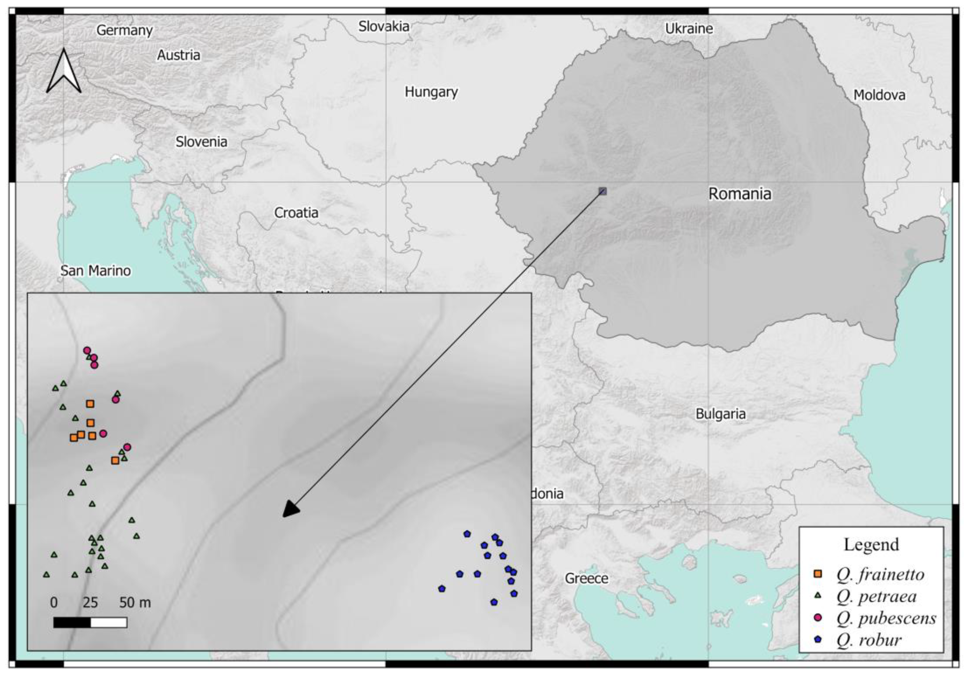
2.1. Study Site

The area that met the requirements for the study was Bejan Oaks’ Reserve. It is a four-oak-species forest located in Romania in the south west of Transylvania near Deva City, in Silvașului Hill, on the left side of the Mureș River (Figure 1). The maximum elevation of the area is 490 m and the minimum elevation is 230 m. According to forest records, oak trees are about 135 years. old and originate from natural regeneration.

2.2. Materials

Two plots were selected in the Bejan mixed oak forest. One plot is dominated by Q. petraea trees along with another two white oak species. The first plot contains scattered Q. frainetto and Q. pubescens. The second plot is dominated by Q. robur trees. FARO FocusS 70, a scanner made in the USA, based on LiDAR technology and included in the category of Terrestrial Laser Scanners (TLS), was used. This is a 3D scanner of high-speed used for measurements that require recording of details. FocusS 70 Laser Scanner uses laser technology, weighing 4.2 kg it is designed for outdoor applications that require scanning up to 70 m and at an accuracy of +/−1 mm.

The FARO FocusS 70 Laser Scanner uses a rotating mirror to beam around the area that is scanned. The measurement characteristics consist of up to 976,000 repetitions per second. This results in a point cloud made representing the scanner’s environment in a three-dimensional dataset. Later, the point cloud is mentioned as the laser scan or simply scan. To maximize the degree of woody branches reconstructed through the point cloud, the best environmental conditions were chosen in terms of no wind environment, leaf-off trees, and uniform light conditions.

2.3. Method

2.3.1. Field Work

As a sampling design for the scanning process, we used QGIS software to generate a grid of points which was overlapped on the area of interest. The distance between two points was set at 12 m resulting in squares with an area of 0.144 hectares each. After delimitation of the squares, the area of interest was designed as a structure similar to a chess table. Before placing the scanner over the point indicated by GPS the corners of the squares were marked for a better orientation. Based on this structure 33 scans were performed in the field in March 2020 prior to bud burst.

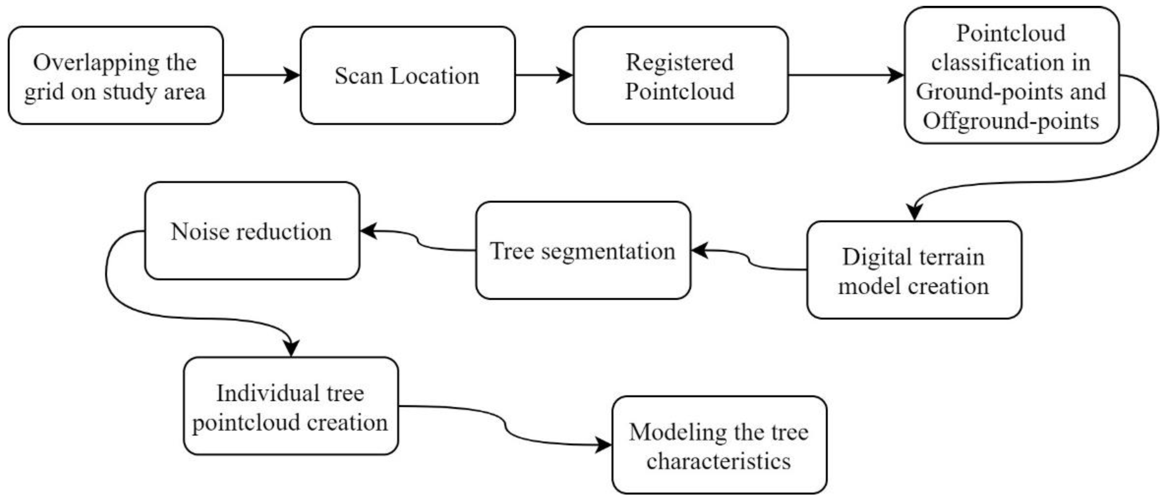
2.3.2. Data Processing and Analysis

After field work, the data was downloaded from the scanner. Data processing and analyzing were realized using six software packages: CloudCompare, 3D Forest, TreeQSM written in MATLAB, QGIS, and R software through RStudio. The first step of data processing consisted in a very precise matching of all scans using the cloud to cloud registration technique. After registration, the entire point cloud was classified in two categories: ground points and off-ground points. We used Cloth Simulation Filter (CSF) to extract ground points in discrete return LiDAR. Ground points define terrain and off-ground points define vegetation over the soil (Figure 2).

After obtaining the off-ground points, each tree was identified and separated from the initial point cloud using a segmentation technique based on top-view projection of the tree. Data cleaning and noise reduction was needed for removal of unwanted bushes and branches.

For the tree woody structure, we used a quantitative structure model (QSM) that provides information about topology (branching structure), geometry, and volume [16]. We used cover sets which are built by splitting the point cloud into small sets that separate the point cloud into trunk and individual branches. Every time a branch is identified, its base is saved as a starting point for the next segmentation. The process starts again with the first order branches and so on, to the last branching order. The branches are identified as possible bifurcations through a local topological analysis of cover sets. The segments should correspond to the real branches and the segmentation process needs corrections to assure this. As a result, the segmentation, the volume reconstruction, the branching structure and order are all different and usually closer to reality [16].

These properties are detailed in terms of total number of branches, the number of branches of a specific order, the parent-child relation between the branches, the length, volume and angles of individual branches, and branch size distribution. The results of QSM are provided as a structure array that contains six different structures as: “cylinder”, “branch”, “pmdistance”, “treedata”, and “triangulation”. These data are the raw information which were then used in calculating the tree characteristics defined in

Table 1. Tree characteristics provided using TreeQSM.

Tree Characteristics	Description
Total Volume	total volume of the tree (sum of all cylinder volumes) in liters
Trunk Volume	volume of the stem in liters
Branch Volume	volume of all the branches in liters
Tree Height	height of the tree in meters vertical distance between the base of the tree and the tip of the highest branch on the tree
Trunk Length	length of the stem in meters between the base of the tree and the tip of the highest branch of the tree
Branch Length	total length of all the branches in meters
Number Branches	number of branches
Max Branch Order	maximum branching order
Total Area	total surface area of the tree in sq.m. (sum of all cylinder surface area)
DBHqsm	DBH in m, the diameter of the cylinder in the QSM at the right height

.

RStudio interface was used for extraction of R² and p-values for all analyzed tree characteristics. For computations, a correlation matrix was used with significance levels (p-value). The function “rcorr” from the package “Hmisc” R package was used to compute the significance levels for Pearson and Spearman correlations for all possible pairs of columns of the matrix. We used the Spearman correlations with a significance level of p-value < 0.05. To easily observe the significant correlations the R package “corrplot” was used to display the correlation matrix. (Appendix A, Figure A1).

2.3.3. Genetic Data Analysis

Genetic data generated in a previous study [33] was used for correlations with tree shape variables. The genetic dataset consisted of ten genomic and EST (expressed sequence tag) nuclear microsatellite markers. Individual heterozygosity was calculated using GenAlEx 6.503 [34]. Oak trees were classified as pollen donor or non-donor based on a paternity analysis performed at Bejan forest [32]. According to this study, pollen donors were identified using highly polymorphic DNA markers. The analysis focused on Q. petraea, the most common species of white oak in Bejan forest. The Mann–Whitney U test was used to compare differences between pollen donors and non-donors. Spearman rank correlation was calculated to assess whether there was any association between male fecundity (i.e., number of observed pollination events) and tree characteristics. Statistica software [35] was used for all calculations.

3. Results

3.1. Scan Registration Accuracy and Point Cloud Statistics

After using cloud to cloud method, the mean point error was 7.7 mm reaching out to a maximum point error of 9.9 mm. The minimum overlap between scans was over 55% and the maximum inclinometer mismatch was 0.053. The point cloud was characterized with a density of approx. 5000 points/sq.m.

Each tree was reconstructed based on an average of 0.25 million 3D points stored in individual point clouds, ranging from 0.1 to 2.2 million points. After noise filtering of all elements smaller than 10 mm, which were discarded to avoid misleading information in the QSM reconstruction, the 3D point clouds of each tree were reduced by an average of approx. 5% of the original data.

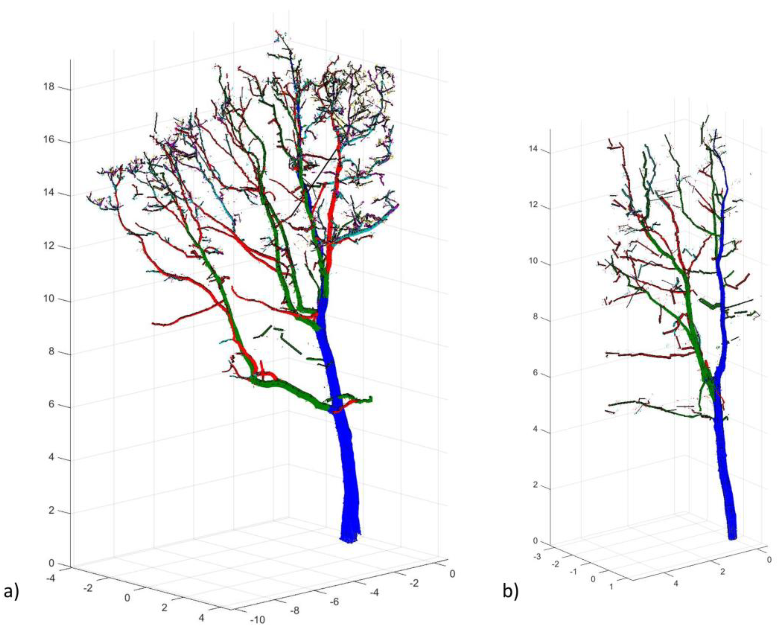
3.2. Tree Shape Variability

A total of 51 individual trees that belong to four oak species were identified from scans: 25 Q. petraea, 6 Q. pubescens, 6 Q. frainetto, and 14 Q. robur. The total volume of trees was 102.16 m³ built from 65% (66.524 m³) trunk volume and 35% (35.635 m³) branch volume. The mean trunk length was larger by approximately 1 m more than the tree height, which is valid for all Quercus species (

Table 2. Trunk and crown characteristics using TreeQSM.

Value	Trunk					Crown
	Total Vol	Trunk Vol	Tree Hgt.	Trunk Len	DBH	Branch Vol	Branch Len	No. Branch	Max Branch Order	Total Area
	m3	m3	m	m	cm	m3	m	-	-	m2
Quercus spp. (51 individuals)
Mean	2.003	1.304	20.015	21.133	45.86	0.699	489.9	615.314	6	62.45
SD	1.323	0.898	3.736	4.7	14.98	0.669	464.1	655.356	2.175	46.74
Q. petraea (25 individuals)
Mean	2.189	1.646	20.746	22.168	51.41	0.542	360.2	459.800	5.400	51.39
SD	1.395	1.010	4.078	4.603	13.76	0.588	397.0	561.001	2.598	39.59
Q. robur (14 individuals)
Mean	1.856	0.953	20.742	21.742	42.73	0.903	631.823	687.571	6.300	78.64
SD	1.049	0.587	3.215	4.946	14.10	0.642	412.894	547.247	1.499	47.62
Q. frainetto (6 individuals)
Mean	2.428	1.264	18.885	19.872	42.18	1.163	899.067	1279.333	6.667	95.33
SD	1.837	0.869	2.274	2.920	17.71	1.015	734.870	1108.775	1.751	68.20
Q. pubescens (6 individuals)
Mean	1.148	0.739	16.402	16.655	33.74	0.410	290.683	430.667	7.000	37.85
SD	0.782	0.458	2.526	3.831	20.30	0.332	159.239	265.82	1.414	20.30

).

Field data revealed that all tree characteristics were significantly correlated with total volume emphasized by a p-value smaller than 0.05. The crown variables were strongly correlated to each other, the branch volume being influenced by branch length, maximum branch order, and the number of branches but not influenced by DBH, trunk length, trunk volume, and tree height (Appendix A, Figure A1). The values of total volume per tree were higher than the general mean, a trend identified also in the case of trunk volume, tree height, and trunk length (Table 2).

Regarding distance between sampled oak trees in the measured stands, according to the Nearest Neighbour Analysis from QGIS Software the average value was 7.57 m. Regarding Q. petraea attributes compared with the mean values the tree height was different with 8%, the trunk volume with 46%, and the total volume with 13%. All values of crown characteristics were lower than the mean value, with 29% for branch volume, 32% for branch length, 32% for number of branches, and the maximum branch order decreased by one order. For Q. robur the mean total volume and the mean DBH was 7% lower than the general mean, while tree height, trunk length, and the maximum branch order were approximately 5% higher than the general mean. The branch volume, branch length, and the total area were almost 30% higher than the general mean. Q. frainetto had the highest volume, its mean total volume per tree was 21% higher than the mean total volume per tree of all oaks. The average volume was divided nearly equally between trunk (52%) and branch volume (48%). Q. pubescens individuals had a much smaller size compared to the other oak species. In most of the cases the stem was not straight, and the results show that consequently trunk length is higher than tree height (Table 2).

We tested tree shape variability between oak species using a Mann–Whitney U test (Appendix B,

Table A2. Mann–Whitney U Test: U, Z, and p-values.

	Q. robur vs. Q. pubescens			Q. robur vs. Q. petraea			Q. robur vs. Q. frainetto
	U	Z	p-Level	U	Z	p-Level	U	Z	p-Level
Total Volume	27	1.237	0.21602	154	−0.615	0.53000	38	−0.412	0.68005
Trunk Volume	33	0.742	0.45790	98.5	−2.240	0.02511	34	−0.660	0.50936
Branch Volume	24	1.485	0.13765	113	1.815	0.06950	37	−0.412	0.68005
Tree Height	10	2.639	0.00831	152	0.673	0.50070	21	1.732	0.08327
Trunk Length	10	2.639	0.00831	165	0.293	0.76960	22	1.650	0.09903
Branch Length	22	1.650	0.09903	100	2.196	0.02811	34	−0.660	0.50936
Number Branches	36	0.495	0.62069	115	1.757	0.07898	26	−1.320	0.18695
Max Branch Order	30.5	−0.949	0.34287	140.5	1.010	0.31247	36	−0.495	0.62069
Total Area	19	1.897	0.05783	121	1.581	0.11389	36	−0.495	0.62069
DBH	25	1.402	0.16088	122	−1.552	0.12074	40	0.165	0.86898
IH	22	−1.650	0.09903	152.5	0.659	0.51007	34.5	0.619	0.53619
	Q. pubescensvs. Q. petraea			Q. pubescensvs. Q. frainetto			Q. petraeavs. Q. frainetto
	U	Z	p-Level	U	Z	p-Level	U	Z	p-Level
Total Volume	33	−2.100	0.03573	11	−1.121	0.26233	75	0.000	1.00000
Trunk Volume	25	−2.500	0.01242	13	−0.801	0.42334	61	0.700	0.48393
Branch Volume	72	0.150	0.88077	10	−1.281	0.20019	41	−1.700	0.08913
Tree Height	26	−2.450	0.01429	8	−1.601	0.10932	49.5	1.275	0.20231
Trunk Length	29	−2.300	0.02145	8.5	−1.521	0.12754	55	1.000	0.31726
Branch Length	66	0.450	0.65271	7	−1.761	0.07817	37	−1.900	0.05744
Number Branches	56	0.950	0.34211	6	−1.922	0.05467	33	−2.100	0.03573
Max Branch Order	47.5	1.375	0.16913	16	0.320	0.74442	54	−1.050	0.28821
Total Area	65	−0.500	0.61708	8	−1.601	0.10932	42	−1.650	0.09894
DBH	22.5	−2.650	0.08665	13	−0.801	0.42334	46	1.450	0.14706
IH	23	2.600	0.09323	5	2.082	0.03216	73	0.100	0.91878

). There were significant differences between Q. robur and Q. pubescens in tree height and trunk length level, between Q. petraea and Q. robur in trunk volume and branch length, between Q. pubescens and Q. petraea in total volume, trunk volume, tree height, trunk length, DBH, as well as between Q. petraea and Q. frainetto in number of branches. The tree shape was not significantly different between Q. frainetto and Q. robur and between Q. frainetto and Q. pubescens.

The influence of the species on all tree characteristics was significant only for trunk volume, tree height, and trunk length, respectively (Appendix B,

Table A3. Kruskal-Wallis ANOVA by RANKS-Kruskal-Wallis test: H.

Trunk and Crown Characteristics	Kruskal-Wallis Test: H
Total Volume m3	(3, N = 51) = 3.955066 p =0.2664
Trunk Volume m3	(3, N = 51) = 8.505381 p =0.0366
Branch Volume m3	(1, N = 20) = 2.204082 p =0.1376
Tree Height	(1, N = 20) = 6.965986 p =0.0083
Trunk Length	(1, N = 20) = 6.965986 p =0.0083
Branch Length	(1, N = 20) = 2.723136 p =0.0989
Number of Branches	(1, N = 20) = 0.244898 p =0.6207
Max Branch Order	(1, N = 20) = 0.942164 p =0.3317
Total Area	(1, N = 20) = 3.598639 p = 0.0578
DBH qsm	(1, N = 20) = 1.965986 p = 0.1609
IH (individual heterozygosity)	(1, N = 20) = 2.838469 p = 0.0920

).

The individual heterozygosity was not significantly correlated with any trunk and crown characteristics. The value of the Spearman coefficient of correlation ranged between –0.16 and 0.13 (Appendix A, Figure A1).

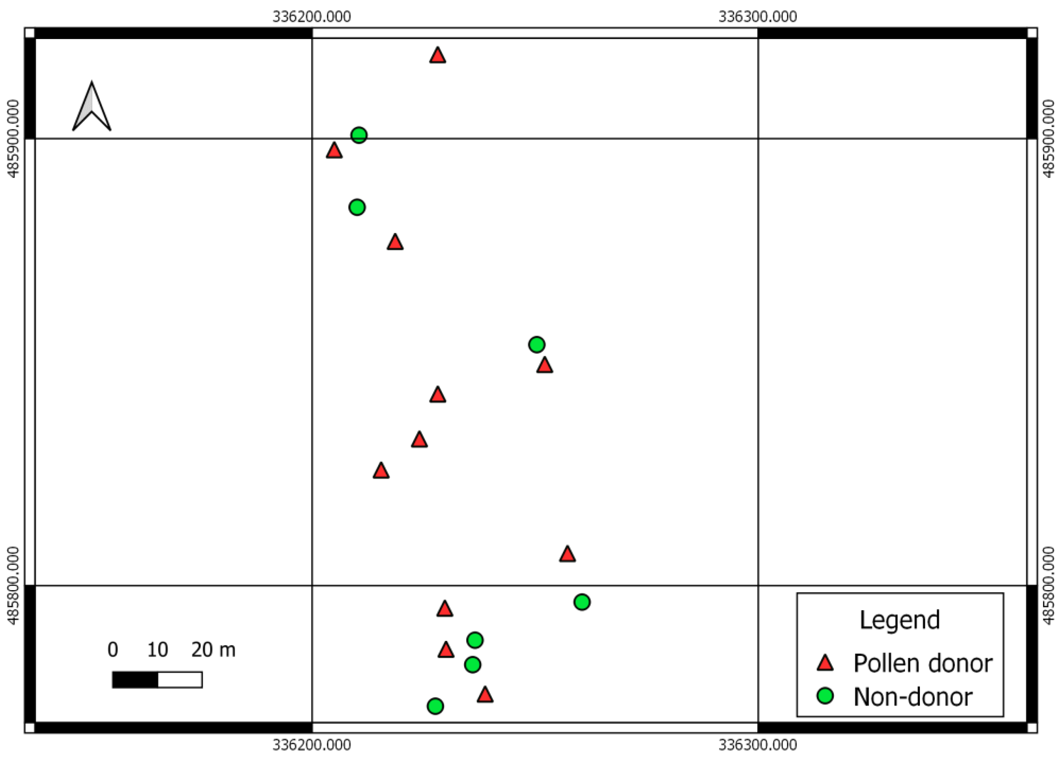
3.3. Tree Shape and Male Fecundity

The individuals of Q. petraea, the most common oak species at Bejan, were split into two categories: pollen donors and non-donors (Figure 3).

A total of 18 Q. petraea individuals were considered in the comparative analysis. Eleven trees were included in the first category (pollen donors) and seven individuals in the second one (non-donors) based on a previous mating system study [32]. The mean distance between the sampled Q. petraea trees was 9.52 m.

Pollen donors showed greater values than non-donor trees for most of the trunk and crown characteristics (

Table 3. Trunk and crown characteristics for pollen donors and non-donors in Q. petraea. p-values for differences between the two categories were calculated with the Mann–Whitney U test.

Trunk						Crown
Category	Total Vol.	Trunk Vol.	Tree Hgt.	Trunk Len.	DBH	Branch Vol.	Branch Len.	No Branches	Max Branch Order	Total Area
	m3	m3	m	m	cm	m3	m	-	-	m2
Pollen Donors
Mean	2.703	1.846	20.409	22.682	53.026	0.857	554.679	723.3	6.5	72.100
SD	1.157	0.889	3.922	4.271	10.532	0.596	421.900	607.0	2.7	38.790
Non-Donors
Mean	1.276	1.039	19.633	20.353	39.553	0.238	179.912	243.4	5	30.272
SD	0.522	0.531	4.129	4.040	9.888	0.918	195.907	304.9	2.3	14.015
p-value	0.010	0.042	0.683	0.556	0.021	0.021	0.052	0.077	0.249	0.027

and Figure 4).

Pollen donors had a larger crown as indicated by the total area and branch volume but a similar height and trunk length with non-donor trees (Figure 4). The difference in the number of branches and branch length between pollen donors and non-donors was marginally non-significant (p = 0.052 and p = 0.077, respectively). There were also significant differences in DBH between the two categories of trees (p = 0.021). However, there was no association between male fecundity as revealed by a paternity analysis [32] and trunk and crown characteristics. The Spearman correlation values were positive in nearly all cases with the highest value for the association with branch length (r = 0.28) (data not shown).

4. Discussion

The architecture developed by an individual tree during the life cycle is the natural reaction of its response to the specific site conditions, particularly in terms of competition, access to light sources, and control of posture against gravity. Understanding the 3D shape of the tree woody biomass is a critical factor in evaluating forest stand environments and evaluating interdependence between trees in terms of competition and mating; however, when using conventional methods, acquiring these data is time consuming and regularly damaging (e.g., field estimates using destructive methods). Measurements that can be achieved especially using Terrestrial LiDAR Scanner (TLS) are fast, practical, complete, and accurate in digitization of individual trees or entire plots. TLS also made estimating the architecture of standing trees in forest ecosystems conceivably complex, with precise assessments of the volume, biomass, or size distribution of branches [15,16,36]. TLS appears as a promising strategy in forested environments, particularly in reconstructing the architecture of singular trees that require a consistent level of data on the structure of the tree branch network [5,37].

We achieved highly accurate dense point clouds which allowed us to reconstruct branches up to level 7, using an innovative approach by combining terrestrial measurements (e.g., appropriate distance and planned positioning of the scan stations), optimal weather conditions (e.g., no wind, constant illumination), and appropriate forest environment status (e.g., leaf-off). The point clouds extracted with TLS revealed additional information to discriminate oak species based on characteristics of the trunk and crown. We found significant differences between different tree characteristics in all four oak species either at trunk, height, or branch level.

Compared with other scanning studies on broadleaved species in Romania [11,12,38] the shape of the oaks is more complex than beech, with a more detailed level on branches especially due to the thickness, allowing a robust reconstruction of branch level even on level 6 or 7.

A similar combination of putatively neutral (genomic SSRs) and potentially adaptive (expressed sequence tag, EST-SSRs) makers as in our study was recently used to analyze the influence of heterozygosity on stem and crown characteristics of Northern red oak in Germany [21]. A significant relationship was only found between branch angle characteristics and individual heterozygosity in Northern red oak. The lack of association between the tree shape characteristics and the measure of genetic diversity (heterozygosity) in the European white oak complex at Bejan Forest may be explained by the small number of DNA regions analyzed, their putative function and location (e.g., in the non-coding part of the genes in case of genomic SSRs). No association between heterozygosity and fitness characteristics was observed in Scots pine [39]. However, the degree of heterozygosity differed significantly between Norway spruce selected clones from a seed orchard and randomly chosen trees in forest stands [40].

Larger trees may have more male catkins and disperse their pollen more effectively. We found differences in crown and trunk characteristics between pollen donors and non-donors identified at Bejan by paternity exclusion using highly polymorphic DNA markers [32]. Pollen donors had larger crown and branch volumes, a higher number of branches, and longer branches. Moreover, there was no significant difference in height between the sampled oak trees, suggesting that all sampled trees at Bejan have the same light accessibility.

One measure of tree size, DBH, was compared to male fecundity in several tree species [22,23]. It was found that DBH is not an important factor influencing male mating success, which is consistent with our finding. However, a positive correlation between DBH and the proportion of fertilizations was observed in one population of Fagus crenata [41]. Nevertheless, crown characteristics such as volume and length of branches may be more important for pollen production than DBH, which is easily measured in the field. Indeed, the relationship between crown volume and effective male fecundity was investigated in a stand of North American oaks [22]. A weak but significant positive correlation was found between the crown volume, estimated based on crown diameter and height, and male fertilization success of oak trees. A weak but non-significant positive association between the number of pollinations and the branch volume was observed in Q. petraea at the Bejan forest. The lack of significance may be explained by the low numbers of effective pollinations detected in the mixed oak forest by paternity exclusion [32]. The acorns were collected in a non-mast year because the distance between consecutive mast years can be 10 or even more years in local oak species [42].

5. Conclusions

The potential of terrestrial laser scanning to assess trunk and crown characteristics in various European white oak species was demonstrated. It proves to be a powerful tool for characterizing the tree phenotype in the era of genomics. Even though there was no association between our set of genetic makers and the tree phenotype, further studies should explore the relationship by considering more specific gene regions. Terrestrial laser scanning may contribute to a better understanding of mating system patterns in oak forests. Combined with floral phenology observations (e.g., based on remote sensing technology) very precise information on tree shape can be of great help in interpreting mating dynamics in forest stands.

References

1. Pretzsch, H. Canopy space filling and tree crown morphology in mixed-species stands compared with monocultures. For. Ecol. Manag. 2014, 327, 251–264. [Google Scholar] [CrossRef] [Green Version]
2. Chen, H.Y.H.; Klinka, K.; Kayahara, G.J. Effects of light on growth, crown architecture, and specific leaf area for naturally established Pinus contorta var. latifolia and Pseudotsuga menziesii var. glauca saplings. Can. J. For. Res. 1996, 26, 1149–1157. [Google Scholar] [CrossRef]
3. Forrester, D.I.; Benneter, A.; Bouriaud, O.; Bauhus, J. Diversity and competition influence tree allometric relationships—Developing functions for mixed-species forests. J. Ecol. 2017, 105, 761–774. [Google Scholar] [CrossRef] [Green Version]
4. Jensen, E.C.; Long, J.N. Crown structure of a codominant Douglas-fir (Pseudotsuga menziesii). Can. J. For. Res. 1983, 13, 264–269. [Google Scholar] [CrossRef]
5. Lau, A.; Bentley, L.P.; Martius, C.; Shenkin, A.; Bartholomeus, H.; Raumonen, P.; Malhi, Y.; Jackson, T.; Herold, M. Quantifying branch architecture of tropical trees using terrestrial LiDAR and 3D modelling. Trees Struct. Funct. 2018, 32, 1219–1231. [Google Scholar] [CrossRef] [Green Version]
6. Van der Zande, D.; Hoet, W.; Jonckheere, I.; van Aardt, J.; Coppin, P. Influence of measurement set-up of ground-based LiDAR for derivation of tree structure. Agric. For. Meteorol. 2006, 141, 147–160. [Google Scholar] [CrossRef]
7. Murray, J.; Fennell, J.T.; Blackburn, G.A.; Whyatt, J.D.; Li, B. The novel use of proximal photogrammetry and terrestrial LiDAR to quantify the structural complexity of orchard trees. Precis. Agric. 2020, 21, 473–483. [Google Scholar] [CrossRef] [Green Version]
8. Garms, C.G.; Simpson, C.H.; Parrish, C.E.; Wing, M.G.; Strimbu, B.M. Assessing lean and positional error of individual mature douglas-fir (Pseudotsuga menziesii) trees using active and passive sensors. Can. J. For. Res. 2020, 50, 1228–1243. [Google Scholar] [CrossRef]
9. Zhou, T.; Popescu, S.; Lawing, A.; Eriksson, M.; Strimbu, B.; Bürkner, P. Bayesian and Classical Machine Learning Methods: A Comparison for Tree Species Classification with LiDAR Waveform Signatures. Remote Sens. 2017, 10, 39. [Google Scholar] [CrossRef] [Green Version]
10. Holopainen, M.; Vastaranta, M.; Kankare, V.; Räty, M.; Vaaja, M.; Liang, X.; Yu, X.; Hyyppä, J.; Hyyppä, H.; Viitala, R.; et al. Biomass estimation of individual trees using stem and crown diameter TLS measurements. ISPRS Int. Arch. Photogramm. Remote Sens. Spat. Inf. Sci. 2012, 3812, 91–95. [Google Scholar] [CrossRef] [Green Version]
11. Pascu, I.S.; Dobre, A.C.; Badea, O.; Tănase, M.A. Estimating forest stand structure attributes from terrestrial laser scans. Sci. Total Environ. 2019, 691, 205–215. [Google Scholar] [CrossRef] [PubMed]
12. Apostol, B.; Chivulescu, S.; Ciceu, A.; Petrila, M.; Pascu, I.S.; Apostol, E.N.; Leca, S.; Lorent, A.; Tanase, M.; Badea, O. Data collection methods for forest inventory: A comparison between an integrated conventional equipment and terrestrial laser scanning. Ann. For. Res. 2018, 61, 189–202. [Google Scholar] [CrossRef]
13. Nita, M.D.; Clinciu, I.; Popa, B. Evaluation of stream bed dynamics from Vidas torrential valley using terrestrial measurements and GIS techniques. Environ. Eng. Manag. J. 2016, 15, 1387–1395. [Google Scholar] [CrossRef]
14. Tang, S.; Dong, P.; Buckles, B.P. Three-dimensional surface reconstruction of tree canopy from lidar point clouds using a region-based level set method. Int. J. Remote Sens. 2013, 34, 1373–1385. [Google Scholar] [CrossRef]
15. Seidel, D. A holistic approach to determine tree structural complexity based on laser scanning data and fractal analysis. Ecol. Evol. 2018, 8, 128–134. [Google Scholar] [CrossRef]
16. Raumonen, P.; Kaasalainen, M.; Åkerblom, M.; Kaasalainen, S.; Kaartinen, H.; Vastaranta, M.; Holopainen, M.; Disney, M.; Lewis, P. Fast Automatic Precision Tree Models from Terrestrial Laser Scanner Data. Remote Sens. 2013, 5, 491–520. [Google Scholar] [CrossRef] [Green Version]
17. Hackenberg, J.; Morhart, C.; Sheppard, J.; Spiecker, H.; Disney, M. Highly Accurate Tree Models Derived from Terrestrial Laser Scan Data: A Method Description. Forests 2014, 5, 1069–1105. [Google Scholar] [CrossRef] [Green Version]
18. Krůček, M.; Král, K.; Cushman, K.; Missarov, A.; Kellner, J.R. Supervised Segmentation of Ultra-High-Density Drone Lidar for Large-Area Mapping of Individual Trees. Remote Sens. 2020, 12, 3260. [Google Scholar] [CrossRef]
19. White, T.L.; Adams, W.T.; Neale, D.B. Forest Genetics; CABI Publishing: Wallingford, UK, 2007; ISBN 1845932854. [Google Scholar]
20. Müller-Starck, G. Genetic differences between “tolerant” and “sensitive” beeches (Fagus sylvatica L.) in an environmentally stressed adult forest stand. Silvae Genet. 1985, 34, 241–247. [Google Scholar]
21. Burkardt, K.; Pettenkofer, T.; Ammer, C.; Gailing, O.; Leinemann, L.; Seidel, D.; Vor, T. Influence of heterozygosity and competition on morphological tree characteristics of Quercus rubra L.: A new single-tree based approach. New For. 2020, 1–17. [Google Scholar] [CrossRef]
22. Dow, B.D.; Ashley, M. V High levels of gene flow in bur oak revealed by paternity analysis using microsatellites. J. Hered. 1998, 89, 62–70. [Google Scholar] [CrossRef] [Green Version]
23. Chybicki, I.J.; Burczyk, J. Seeing the forest through the trees: Comprehensive inference on individual mating patterns in a mixed stand of Quercus robur and Q. petraea. Ann. Bot. 2013, 112, 561–574. [Google Scholar] [CrossRef] [Green Version]
24. Barrett, S.; Kohn, J. Genetic and evolutionary consequences of small population size in plants: Implications for conservation. In Genetics and Conservation of Rare Plants; Oxford University Press: New York, NY, USA, 1991; pp. 3–30. [Google Scholar]
25. Franceschinelli, E.V.; Bawa, K.S. The effect of ecological factors on the mating system of a South American shrub species (Helicteres brevispira). Heredity 2000, 84, 116–123. [Google Scholar] [CrossRef] [Green Version]
26. Farris, M.A.; Mitton, J.B. Population density, outcrossing rate, and heterozygote superiority in ponderosa pine. Evolution 1984, 38, 1151–1154. [Google Scholar] [CrossRef] [PubMed]
27. Schmitt, J. Density-dependent pollinator foraging, flowering phenology, and temporal pollen dispersal patterns in Linanthus bicolor. Evolution 1983, 37, 1247–1257. [Google Scholar] [CrossRef] [PubMed]
28. Ennos, R.A.; Clegg, M.T. Effect of population substructuring on estimates of outcrossing rate in plant populations. Heredity 1982, 48, 283–292. [Google Scholar] [CrossRef] [Green Version]
29. Menitsky, Y.L. Oaks of Asia; CRC Press: Boca Raton, FL, USA, 2005. [Google Scholar]
30. Johnson, P.S.; Shifley, S.R.; Rogers, R. The Ecology and Silviculture of Oaks; CABI Publishing: Wallingford, UK, 2002. [Google Scholar]
31. Nixon, K.C. Infrageneric classification of Quercus (Fagaceae) and typification of sectional names. Ann. Des. Sci. For. 1993, 50, 25–34. [Google Scholar] [CrossRef] [Green Version]
32. Curtu, A.L.; Gailing, O.; Finkeldey, R. Patterns of contemporary hybridization inferred from paternity analysis in a four-oak-species forest. BMC Evol. Biol. 2009, 9, 284. [Google Scholar] [CrossRef] [Green Version]
33. Curtu, A.L.; Craciunesc, I.; Enescu, C.M.; Vidalis, A.; Sofletea, N. Fine-scale spatial genetic structure in a multi-oak-species (Quercus spp.) forest. iForest Biogeosci. For. 2015, 8, 324–332. [Google Scholar] [CrossRef] [Green Version]
34. Peakall, R.O.D.; Smouse, P.E. GENALEX 6: Genetic analysis in Excel. Population genetic software for teaching and research. Mol. Ecol. Notes 2006, 6, 288–295. [Google Scholar] [CrossRef]
35. StatSoft STATISTICA for Windows, Version 8.0; Software-System for Data Analysis; StatSoft, Inc.: Tulsa, OK, USA, 2008.
36. Li, Y.; Su, Y.; Zhao, X.; Yang, M.; Hu, T.; Zhang, J.; Liu, J.; Liu, M.; Guo, Q. Retrieval of tree branch architecture attributes from terrestrial laser scan data using a Laplacian algorithm. Agric. For. Meteorol. 2020, 284. [Google Scholar] [CrossRef]
37. Ferrara, R.; Virdis, S.G.P.; Ventura, A.; Ghisu, T.; Duce, P.; Pellizzaro, G. An automated approach for wood-leaf separation from terrestrial LIDAR point clouds using the density based clustering algorithm DBSCAN. Agric. For. Meteorol. 2018, 262, 434–444. [Google Scholar] [CrossRef]
38. Coșofreț, C.; Barnoaiea, I.; Scriban, R.E.; Dănilă, I.C.; Duduman, M.L.; Bouriaud, O. Utilizarea scanerului laser terestru în măsurătorile forestiere: Cerințe metodologice și precauții necesare la aplicarea în practică. Bucov. For. 2018, 18, 137–153. [Google Scholar] [CrossRef]
39. Savolainen, O.; Hedrick, P. Heterozygosity and fitness: No association in Scots pine. Genetics 1995, 140, 755–766. [Google Scholar] [CrossRef]
40. Bergmann, F.; Ruetz, W. Isozyme genetic variation and heterozygosity in random tree samples and selected orchard clones from the same Norway spruce populations. For. Ecol. Manag. 1991, 46, 39–47. [Google Scholar] [CrossRef]
41. Asuka, Y.; Tani, N.; Tsumura, Y.; Tomaru, N. Development and characterization of microsatellite markers for Fagus crenata Blume. Mol. Ecol. Notes 2004, 4, 101–103. [Google Scholar] [CrossRef]
42. Șofletea, N.; Curtu, L. Dendrologie; Editura Universitatii Transilvania: Brasov, Romania, 2007; ISBN 9789736358852. [Google Scholar]
Figure 1. Study area and spatial distribution of sampled oak species.
Forests 12 00253 g001
Figure 2. Processing workflow.
Forests 12 00253 g002
Figure 3. Spatial distribution of pollen donor and non-donor Q. petraea individuals.
Forests 12 00253 g003
Figure 4. Example of donor (a) and non-donor (b) tree of Q. petraea.
Forests 12 00253 g004