Analysis of Factors Influencing Forest Loss in South Korea: Statistical Models and Machine-Learning Model

Abstract

Analyzing the current status of forest loss and its causes is crucial for understanding and preparing for future forest changes and the spatial pattern of forest loss. We investigated spatial patterns of forest loss in South Korea and assessed the effects of various factors on forest loss based on spatial heterogeneity. We used the local Moran’s I to classify forest loss spatial patterns as high–high clusters, low–low clusters, high–low outliers, and high–low outliers. Additionally, to assess the effect of factors on forest loss, two statistical models (i.e., ordinary least squares regression (OLS) and geographically weighted regression (GWR) models) and one machine-learning model (i.e., random forest (RF) model) were used. The accuracy of each model was determined using the R², RMSE, MAE, and AICc. Across South Korea, the forest loss rate was highest in the Seoul–Incheon–Gyeonggi region. Moreover, high–high spatial clusters were found in the Seoul–Incheon–Gyeonggi and Daejeon–Chungnam regions. Among the models, the GWR model was the most accurate. Notably, according to the GWR model, the main factors driving forest loss were road density, cropland area, number of households, and number of tertiary industry establishments. However, the factors driving forest loss had varying degrees of influence depending on the location. Therefore, our findings suggest that spatial heterogeneity should be considered when developing policies to reduce forest loss.

1. Introduction

The global forested area is 4.06 billion ha, which accounts for approximately 31% of the total land area; global forest loss since the 1990s has reached approximately 0.42 billion ha [1]. Forest loss increases ground surface temperatures, reduces ecosystem services, and exacerbates climate change [2]. Climate change is caused by factors such as construction and transportation [3,4]. Forest loss can be driven by human activity and biophysical characteristics (i.e., roads, construction, expansion of settlements, industry, wildfires, agricultural activities, mining, industrial logging, etc.) that directly affect forests and cause canopy loss [5]. In particular, the expansion of urban infrastructures, such as roads, transportation, and settlements, causes permanent forest loss [6,7]. Additionally, demand for forest products and the conversion of native forests into commercial forests can simplify forest vegetation structure and reduce biodiversity [8,9]. Therefore, reducing forest loss is necessary to restore and improve the function of forests [10].

In South Korea, the ratio of forest area is about 63%, which is the fourth highest among OECD countries, following Finland, Sweden, and Japan, with a high forest area ratio compared to the global average forest area ratio [11]. However, the forest cover decreased by approximately 3% in 2019 compared to in 1990, with a mean annual decline of 0.1% [12]. This is a higher figure than the 1.7% decrease in the global forest area ratio over the past 30 years, so it is necessary to reduce it by analyzing the causes of forest loss [1]. According to Kim and Hwang, continuous damage to the forest in South Korea has been reported due to tourist sites, golf courses, industrial complexes, housing areas, road construction, and various other factors [13]. To decrease the rate of forest loss, it is necessary to quantitatively analyze the area of forest loss. Additionally, human socioeconomic factors associated with forest loss need to be determined [14]. Recent improvements to geographic information system (GIS) and remote sensing (RS) tools have enabled the rapid collection of data regarding regional forest conversion and loss [15]. The collected data can be analyzed using various techniques, including statistical approaches and machine-learning models, to examine the spatial distribution characteristics of forest loss and the causes of forest loss [16]. Forest loss can occur due to the conversion of forest to many different land uses, and this process is affected by various spatial and socioeconomic factors. Verburg et al. [17] showed that road construction increases human movement and economic activities, which increases the conversion of forest to croplands and grasslands. Damnyag et al. [18] found that, in Ghana, croplands affected forest loss. Scullion et al. [19] pointed out that pasture expansion is the direct cause of forest loss worldwide, with the causes varying among each continent. Echeverria et al. [20] showed that forests closer to rivers were more likely to be lost. Forest in lower altitudes is less accessible; therefore, forest loss is less likely to occur. Similarly, Gayen and Saha [21] showed that forest with a higher slope is less accessible and less likely to experience forest loss. Sharma et al. [22] showed that commercial land use (mining and transportation development) and infrastructure development increased forest loss due to the expansion of surrounding urban areas.

Given that the factors mentioned above vary spatially [23,24,25], their spatial heterogeneity should be considered when determining their impact on forest loss [26,27]. Therefore, the spatial distribution of forest loss and the relationship between forest loss and its occurrence factors should be analyzed. Regional spatial patterns of forest cover can be quantitatively analyzed using the local Moran’s I, first proposed by Anselin [28]. This technique enables statistically significant spatial clusters and outliers to be measured according to characteristics of the forest loss rate of a given area to quantitatively determine the forest loss rate [29]. Correlations between forest loss and various factors have been conducted using statistical models (e.g., ordinary least squares regression (OLS) and geographically weighted regression (GWR) models) and machine-learning model (e.g., random forest (RF) model) [30,31,32]. The OLS model does not consider the spatial heterogeneity of the area when analyzing correlations among factors, whereas GWR incorporates spatial heterogeneity and, therefore, can provide useful visual information to identify factors impacting forest loss [33]. The GWR model estimates discrete parameters by providing the higher weighted value closer to the observation location [34]. The RF model does not consider spatial heterogeneity; they are similar to the OLS model that provides a single result for the entire range of the research area with high predictive accuracy and efficiency [35,36]. However, the RF model can be used for both classification and regression, which is advantageous for obtaining results very quickly [37]. Nevertheless, the OLS and RF models have rarely been applied to analyze the factors affecting forest loss in South Korea.

In this study, we analyzed the areas of forest loss in South Korea and the factors driving this forest loss. The specific goals were as follows: (1) The distribution of the forest loss area was analyzed using local Moran’s I. (2) The suitability of models (OLS, GWR, and RF) to evaluate factors affecting the forest loss rate was compared. (3) Factors affecting forest loss in each region were analyzed. Understanding the causes of forest loss and forest distribution status may contribute to the development of measures that prevent forest loss. In the future, this study can be used to establish forest management policies to prevent forest loss.

2. Materials and Methods

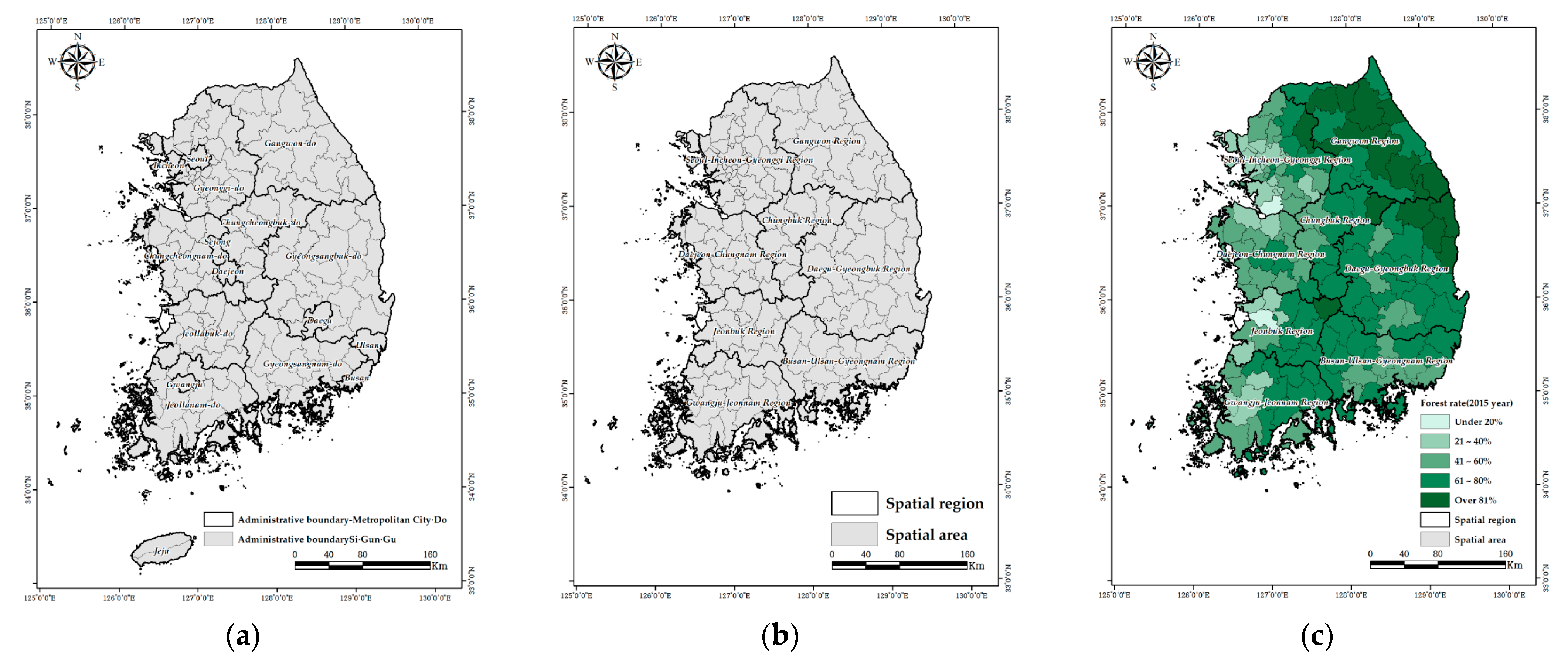
2.1. Study Site

The study was conducted in South Korea at 125°–131° longitude and 33°–38° latitude and included administrative districts, as well as one special city, one special self-governing city, six metropolitan cities, eight provinces, and one special self-governing province. The total area of the study site comprised approximately 10.04 million ha with 63% forest. The highest forest area % of land area was in the Gangwon region (81%), followed by the Daegu–Gyeongbuk (69%) and Busan–Ulsan–Gyeongnam (65%) regions. Forests in the north and east were generally at higher altitudes, and those in the west and south were generally at lower altitudes; however, there were substantial variations in the mean altitude and slope [38]. The study site was divided into eight “spatial regions” containing 152 “spatial areas”, based on eight provinces to which each of the seven metropolitan cities belonged (

Table 1. Number of spatial areas and forest rate in each spatial region. For the study, “spatial regions” were defined and split into “spatial areas” (see Figure 1).

Spatial Region	Seoul–Incheon–Gyeonggi Region	Gangwon Region	Busan– Ulsan– Gyeongnam Region	Daegu Gyeongbuk Region	Gwangju– Jeonnam Region	Jeonbuk Region	Daejeon– Chungnam Region	Chungbuk Region
Spatial area (n)	32	15	20	22	22	14	16	11
Forest rate (%)	46	81	65	69	54	51	51	64

and Figure 1). To analyze forest loss and the factors impacting forest loss from a macroscopic perspective, spatial regions were defined by classifying metropolitan cities and provinces by region. Then, for a more detailed analysis, spatial areas were defined to analyze Seoul and other metropolitan cities and the special self-governing city under the same parameters as those used for general cities. Each spatial area was quantitatively analyzed as an independent unit, irrespective of the size of the cities or provinces. Additionally, Seogwipo-si, Jeju-si in the Jeju Special Self-Governing Province, and Ulleung-gun in Gyeongsangbuk-do, which are geographically remote islands, were excluded from analysis because they are distant from other regions, limiting the weighting in spatial pattern analysis [39]. Furthermore, Sejong Special Autonomous City, an administrative district designated in 2012, was excluded from the analysis due to a lack of statistical data from 2005 [40,41].

2.2. Data Collection

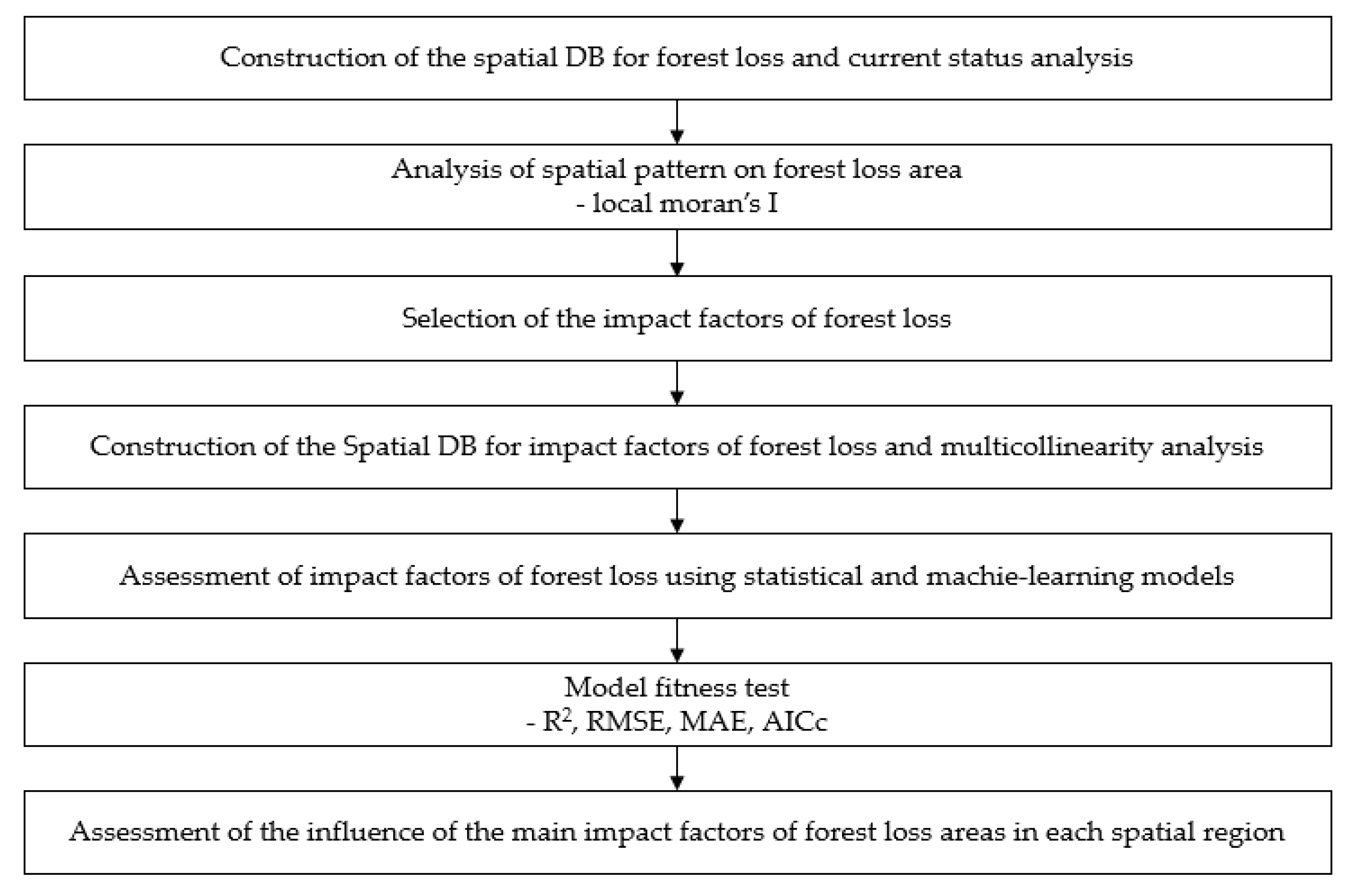
The data used in the status analysis of the spatial distribution of forest loss areas were obtained from the Forest Basic Statistics (FBS), which provides statistics on the current status of national forests in South Korea [42,43]. The FBS data included information regarding the forest type (coniferous forest, deciduous forest, or mixed forest) and age [44,45]. The FBS data are published every five years; the 2015 and 2005 data were used to analyze changes in forest cover over a ten-year period. Census data and spatial data were used to determine factors affecting forest loss. Census data were obtained from the Cadastral Statistics Chronology [46,47]; the Agricultural Area Survey and the Agriculture, Forestry and Fishery Survey [48,49,50,51]; and the Survey of Establishments [52,53]. Spatial data were obtained from the road network map and the railway network map, which were produced in 2005 and 2015 by the Ministry of Land, Infrastructure and Transport (MOLIT). The Cadastral Statistics Chronology includes the area of 28 land categories, including forests, crop fields, paddies, and house sites, for each administrative district [54]. The Agricultural Area Survey provides data on the current status of agricultural land and cultivation within a selected sample area. The Agriculture, Forestry and Fishery Survey analyzes the distribution of agriculture, forestry, and fishery households, number of household members, and farms to construct the data in a cycle of one year and five years [55,56,57]. The Survey of Establishments collects annual data of each region’s establishments, such as size, distribution, industry type, and employees [58]. The road and railway network maps provide the current status of roads and railways across the nation [59] (

Table 2. Sources of data for factors affecting forest loss.

Category	Data	Institution	Year of Data Collection	Detailed Data
Census Data	Forest Basic Statistics	Korea Forest Service (KFS)	2005, 2015	Forested area, accumulation of standing
	Cadastral Statistics Chronology	Ministry of Land, Infrastructure and Transport (MOLIT)		28 land categories, including Forestry, Dry paddy-field, Paddy-field, and Building site
	Agricultural Area Survey	Statistics Korea (KOSTAT)		Current status of agricultural land
	Agriculture, Forestry and Fishery Survey			Number of household members, and farms
	Survey of Establishments	Ministry of Employment and Labor (MOEL)		Size, distribution of industry, industry type,
Spatial Data	Road network map	MOLIT		Spatial data
	Railway network map

).

2.3. Study Method

In this study, a spatial database was constructed to analyze the forest loss rate for 2005–2015 and the spatial patterns of forest loss. Then, a spatial database for the factors potentially influencing forest loss was constructed. The impact of these factors on forest loss was then analyzed using statistical and machine-learning models (Figure 2).

2.3.1. Construction of the Spatial DB for Forest Loss and Current Status Analysis

For the forest loss area, the data of forest area per spatial area were extracted from the 2005 and 2015 FBS data, and using Equation (1), the rate of change in the forest area was estimated. The rate of change in the forest area was negative (−) if the forest area had decreased, and the negative values were converted into positive (+) values to clearly identify the characteristics of forest loss area, while the spatial areas without a decrease in forest area were excluded from the analysis (Equation (1)).

$$\Delta v_t=\frac{\left(v_t-v_{t-1}\right)}{v_{t-1}}$$

(1)

$\Delta v_t$: Forest loss rate at t time; $v_t$: Forest rate at t time;

$v_{t-1 }$: Forest rate at t − 1 time; $v$: Forest rate.

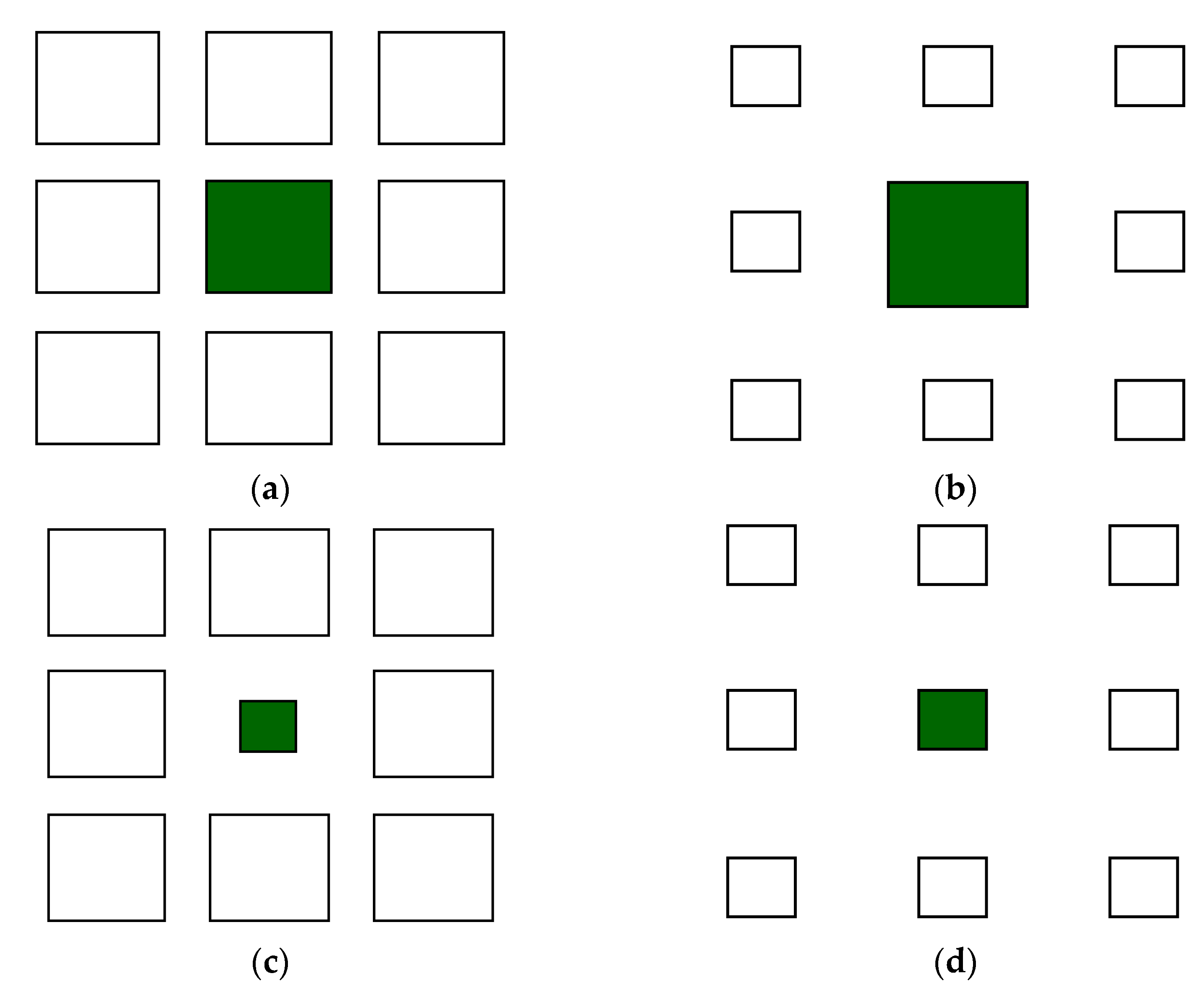
2.3.2. Analysis of Spatial Pattern on Forest Loss Area

The spatial autocorrelation patterns of the forest loss in each area were analyzed using global Moran’s I. A Moran’s I value >0 indicates that the forest loss area is clustered, and a value <0 indicates that the forest loss area is dispersed [60,61] (Equation (2)). The local Moran’s I identifies spatial clusters and outliers based on proximity, which is fundamentally different from the hotspot method but may contribute as a complementary concept because the Moran’s I is a high or low level of similarity to the spatial area in the vicinity [62,63]. In the case of proximity, the Euclidean distance was used to measure the distance between features, and similarity with the neighboring area was analyzed based on the result. Based on this, spatial areas were categorized into the following four spatial patterns: high–high (HH) spatial clusters, high–low (HL) spatial outliers, low–low (LL) spatial clusters, and low–high (LH) spatial outliers (Figure 3) [64]. The local Moran’s I assigns a weight to a given area based on the spatial proximity among the areas in a cluster, and to analyze the consequent patterns, the range and distance of the weight should be determined. We used a fixed bandwidth to determine the weight range of the local Moran’s I in this study [65], and the Euclidean distance was applied for the distance between areas [66,67] (Equation (3)).

$$\mathrm{I}=\frac{n{{\displaystyle \sum }}_{i=1}^n{{\displaystyle \sum }}_{j=1}^n{W}_{ij}\left(d\right)\left(x_i-\overline{x}\right)\left(x_j-\overline{x}\right)}{{{\displaystyle \sum }}_{i=1}^n{{\displaystyle \sum }}_{j=1}^n{W}_{ij}\left(d\right){{\displaystyle \sum }}_i^n{\left(x_i-\overline{x}\right)}^2}$$

(2)

$$I_i=\frac{\left(x_i-\overline{x}\right){{\displaystyle \sum }}_j{W}_{ij}\left(x_j-\overline{x}\right)}{S^2}$$

(3)

$x_i$: forest loss rate at ith area; $x_j : \mathrm{forest}\mathrm{loss}\mathrm{rate}\mathrm{at}j$th$\mathrm{area}$;

$\overline{x}$: the mean of the forest loss rate; $W_{ij} : \mathrm{weight}\mathrm{index}\mathrm{for}\mathrm{the}\mathrm{location}\mathrm{of}i\mathrm{relative}\mathrm{to}j$;

$S^2$: variance; n: number of areas.

2.3.3. Selection of Impact Factors

For the variables that influence forest loss, a total of 11 variables were selected in reference to previous studies conducted in South Korea and overseas (

Table 3. Impact factors of forest loss.

Factor	Description	Unit	Data Source
Road density (Rd)	Forest loss is caused by the increased accessibility due to high road density	m/ha	Mena et al., 2006 [68]
Cropland area (Ca)	Forest loss is caused by the expansion of farms leading to increase in population and poverty	%	Ngwira and Watanbe, 2019 [69]
Grassland area (Ga)	Forest loss is caused by the expansion of industry to meet the increased demand for livestock animals		Walker et al., 2013 [70]
Settlement area (Sa)	Forest loss is caused by the settlement and construction of infrastructure		Jayathilake et al., 2020 [71]
Number of households (Nh)	Forest loss is caused by increase in number of households leading to expansion of croplands	n	Godoy et al., 1997 [72]
Population (P)	Forest loss is caused by increase in population leading to increased demand for food and housing	n	Biswas et al., 2012 [73]
Primary industry number of Employees (Pm)	Forest loss is caused by industrialization and subsequent population pressure	n	Lata et al., 2018 [74]
Primary industry Establishments (Pe)
Secondary industry number of Employees (Sm)
Secondary industry number of Establishments (Se)
Tertiary industry Employees (Tm)
Tertiary industry Establishments (Te)

). The selected variables were as follows: road density [68], cropland area [69], grassland area [70], settlement area [71], number of households [72], population [73], and industry employees and establishments [74]. The “industry employees and establishments” variable was analyzed by first recategorizing the industry types in the Survey of Establishments [52,53] that follows the Fisher–Clark categorization of industry (agriculture, forestry, fishery, mining, manufacturing, electricity, gas and waterwork, transportation, and communication) into primary, secondary, and tertiary industries, then counting the employees and establishments in each class of industry [75]. For each variable, the rate of change for each spatial area was estimated following the same method used to determine changes in forest rate. Next, the multicollinearity of variables was determined, and the variables were excluded from further analyses if the variance inflation factor (VIF) was ≥10 [76].

2.3.4. Concept of Statistical Learning (OLS and GWR Models)

The OLS and GWR models were used to analyze the spatial correlation between forest loss and human activity. The OLS model is a global model that estimates the influence of a given variable as identical across all study areas, based on the assumption that the variables would have identical correlations in any space. Therefore, the OLS model can be used to confirm the influence of variables on the whole study area [77]. Meanwhile, the global correlation determined through the OLS model may deviate from the locally analyzed correlation so that the estimated correlation may differ from the actual correlation [78]. The estimation equations of OLS are shown in Equations (4) and (5). Thus, the OLS model was used to analyze the global impact factors of forest loss.

$$\mathrm{y}={\beta }_0+{{\displaystyle \sum }}_{k=1}^n{\beta }_k{x}_k+\epsilon$$

(4)

$$\widehat{\beta }={\left(X^{\prime }X\right)}^{-1}{X}^{\prime }Y$$

(5)

$\mathrm{y}$: dependent variable; ${\beta }_0$: intercept; ${\beta }_k$: regression coefficient; $x_k$: kth independent variable; $\epsilon$: error; $\widehat{\beta }$: estimated regression coefficient; $X^{\prime }$: transpose matrix of variable;$X$: matrix of variable; $Y$: vector of the dependent variable.

The GWR model allows for estimation of local parameters as a regional model, enabling estimation of the influence of variables by region. In contrast to the OLS model, the influence of the variable within the study area was estimated per area, and the results of the model were applied to each area [79]. This suggests that the GWR produces a more reliable performance than the OLS because local influences are analyzed to allow the study of spatial migration of variables and as the influence is analyzed per area [80,81]. The weight in the GWR model is assigned through kernel functions based on distance [82]. The bandwidth is divided into fixed and adaptive kernels based on how the bandwidth is set as the weight range. For a fixed kernel, the distribution shows bandwidths of consistent size. For adaptive kernels, the distribution varies according to the data density [83]. The weights were assigned via an adaptive kernel. The estimation equations for the GWR are shown in Equations (6)–(8). Thus, the GWR model was used to analyze the impact factors of forest loss in the dimension of areas (units of spatial areas).

$$y_i={\beta }_0\left(u_i, v_i\right)+{{\displaystyle \sum }}_{k=1}^n{\beta }_k\left(u_i, v_i\right)x_{ki}+{\epsilon }_i$$

(6)

$${\widehat{\beta }}_i={\left(X^{\prime }{W}_{i}X\right)}^{-1}{X}^{\prime }{W}_{i}Y$$

(7)

$$w\left(u_i, v_i\right)=\left(\begin{array}{ccc}{w}_{i1}& \cdots & 0\\ ⋮& \ddots & ⋮\\ 0& \cdots & w_{ik}\end{array}\right)$$

(8)

${\beta }_0$: intercept; ${\beta }_k$: estimate coefficient for independent variable; $y_i$: dependent variable; $x_k$: kth independent variable; $\left(u_i, v_i\right)$: longitude and latitude coordinates of ith area; ${\beta }_k\left(u_i, v_i\right)$: estimate coefficient for the location of ith area; ${\epsilon }_i$: error;${\widehat{\beta }}_i$: estimated coefficient for the location of ith area; $X^{\prime }$: transpose matrix of variable;$X$: matrix of variable; $Y$: vector of the dependent variable; $W_i$: weighted matrix for the location of ith area

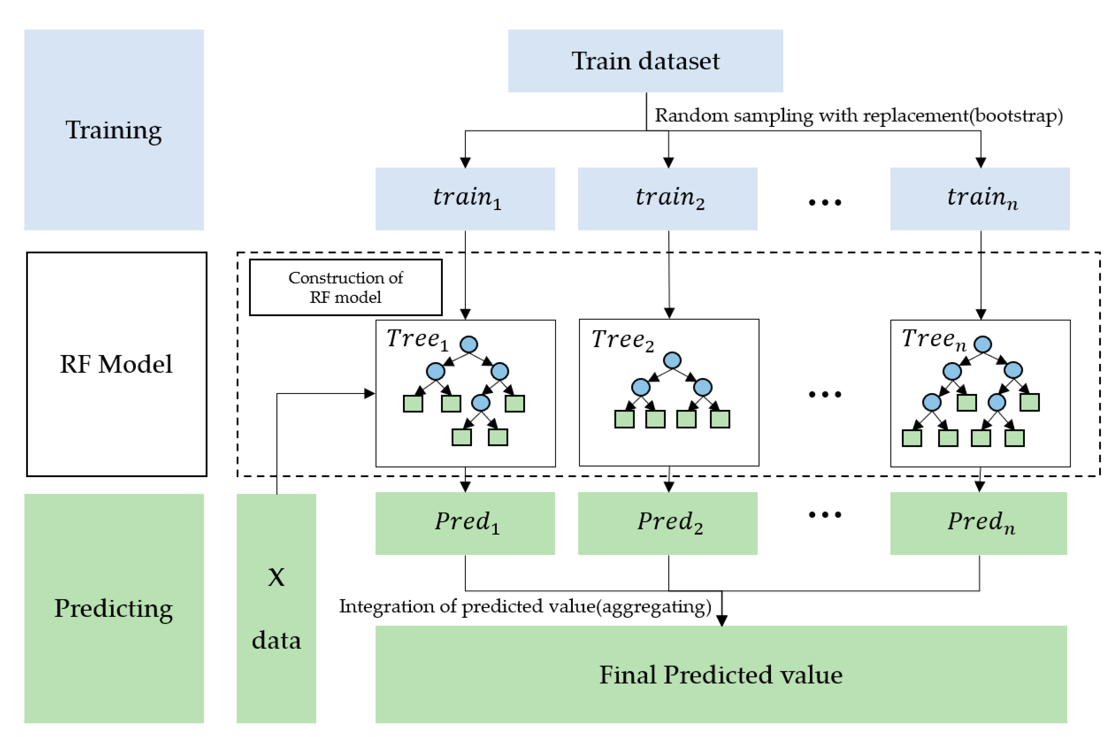
2.3.5. Machine-Learning Model (RF Model)

The performance of a machine-learning model and importance of each impact factor were estimated with respect to forest loss for a comparative analysis concept of statistical learning. The RF model was used because it is a representative machine-learning model which is well-known for its simplicity and efficiency [84]. The RF model was implemented using Python’s scikit-learn library. A variable is selected at each node, and randomness is exhibited by the learning data at each tree to create an ensemble model of myriads of decision trees [85]. In general, the prediction accuracy and efficiency of the RF model are high, with a low probability of overfitting for learning data [35,86]. The RF model was analyzed using n_estimators, max_depth, min_samples_split, and min_samples_leaf as hyperparameters, as shown in

Table 4. Hyperparameters of the random forest (RF) model.

Hyperparameter	Value
n_estimators	100
Max_depth	None
Min_sample_split	2
Min_samples_leaf	1

. n_estimators is the number of regression trees in the model. As n_estimators increases, the fitting effect decreases; therefore, n_estimators is often set to 100 [87]. In addition, in reference to previous studies which reported the use of the basic hyperparameter values leading to a high level of accuracy, n_estimators was set as 100, min_samples_split as 2, max_depth as 0, and min_samples_leaf as 1 [88,89] (Figure 4). We analyzed the hyperparameter as the default value by referring to previous research when evaluating the relationship between dependent and independent variables as well as statistical models [88] (Table 4).

2.3.6. Model Fitness

The coefficient of determination (R²), root mean squared error (RMSE), mean absolute error (MAE), and Akaike’s information corrected criterion (AICc) were used to test the performance of the statistical and machine-learning models. The R² was used to analyze the predictive power of the models. RMSE is a scale that represents the differences between the model-predicted values and the actual observed values and is used to evaluate the accuracy of spatial analyses and remote sensing with error distributions [90,91]. MAE is the mean value for the absolute difference between the model-predicted value and actual value, which indicates the mean error size. As in the RMSE, smaller estimates indicate smaller errors, which verifies a higher prediction accuracy [92,93]. AICc allows the estimation of the relative quantity of data lost in the statistical model. Smaller values indicate a higher model fitness. In general, AICc provides the solution to overfitting when the sample size is small; thus, it is more useful than AIC [94]. The R², RMSE, MAE, and AICc values were obtained using Equations (9)–(12), respectively. Additionally, the influence and importance of variables were analyzed based on the regression coefficients from the statistical models and the IncMSE from the machine-learning model. The regression coefficient is indicative of the influence of the impact of factors on forest loss, and a positive or negative value indicates a positive or negative, respectively [95]. The % IncMSE is indicative of an increase in the mean squared error, and a higher value indicates a more critical variable within the RF model [96].

$${\mathrm{R}}^2=1-\frac{{{\displaystyle \sum }}_{i=1}^n(y_i-\widehat{y_i})}{{{\displaystyle \sum }}_{i=1}^n{(y_i-\overline{y})}^2}$$

(9)

$$\mathrm{RMSE}=\sqrt{\frac{1}{n}{{\displaystyle \sum }}_{i=1}^n{(y_i-\widehat{y_i})}^2}$$

(10)

$$\mathrm{MAE}=\frac{1}{n}{{\displaystyle \sum }}_{i=1}^n\left|y_i-\widehat{y_i}\right|$$

(11)

$$\mathrm{AICc}=2{\mathrm{nlog}}_e\left(\widehat{\sigma }\right)+{\mathrm{nlog}}_e\left(2\pi \right)+n\left(\frac{n+tr\left(s\right)}{n-2-tr\left(s\right)}\right)(S=\frac{\widehat{y_i}}{y_i})$$

(12)

$y_i$: dependent variable; $\widehat{y_i}$: estimated value of dependent variables; $\overline{y_i}$: mean of dependent variables;$\sigma :\mathrm{residual}\mathrm{standard}\mathrm{error}$; $\widehat{\sigma }$: estimated value of residual standard error; $n$: number of variables; tr(s): trace of the hat matrix.

3. Results and Discussion

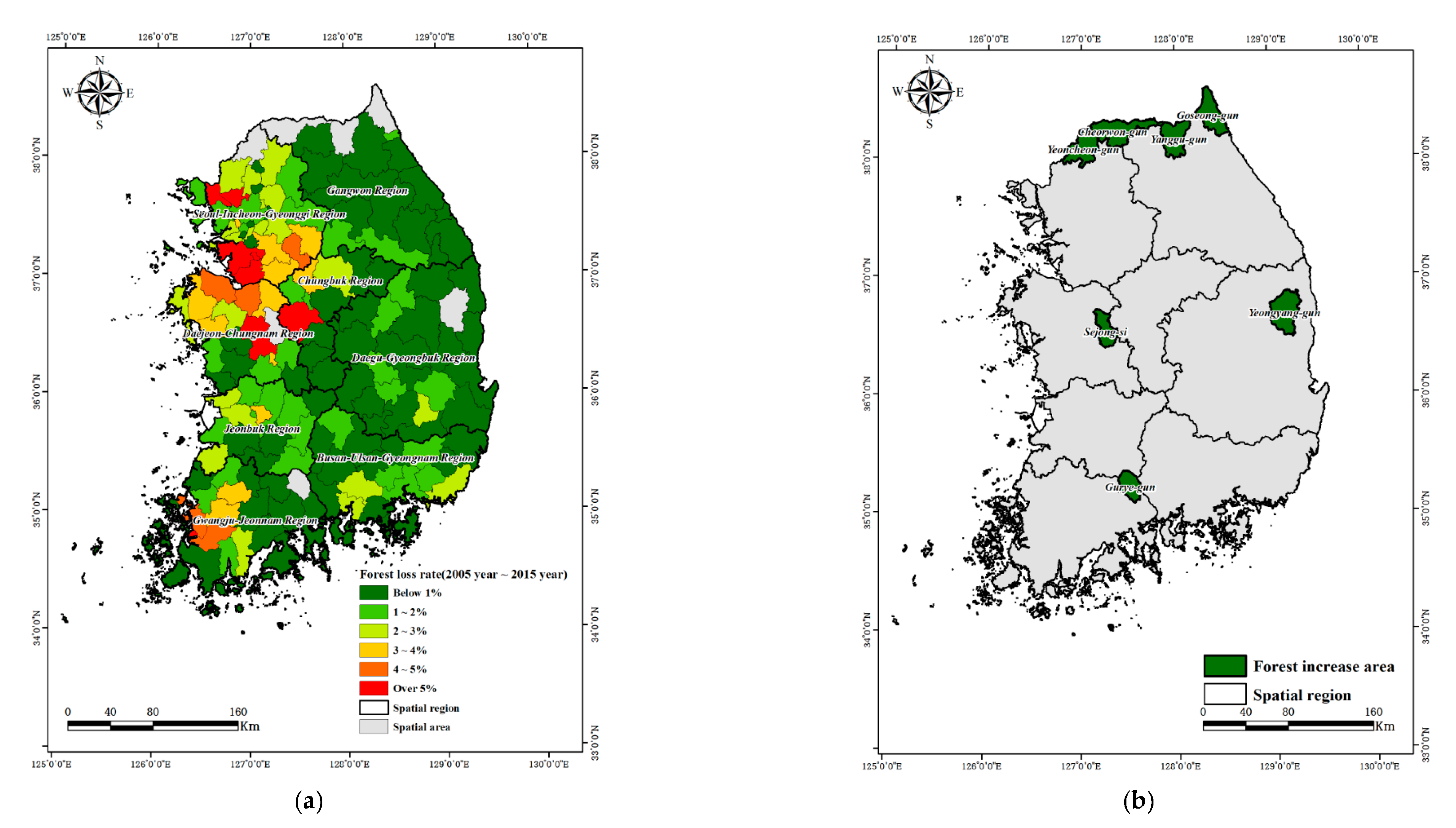
3.1. Spatial Distribution of Forest Loss during 2005–2015

The forest rate in South Korea decreased by approximately 1% in 2015 compared to 2005, with significant differences among spatial regions. The highest forest loss rate was observed in the Seoul–Incheon–Gyeonggi region, and the lowest forest loss rate was observed in the Gangwon region (

Table 5. Distribution of forest loss rate across spatial regions.

Category	Minimum Forest Loss Rate	Mean Forest Loss Rate	Maximum Forest Loss Rate	Standard Deviation
Seoul–Incheon–Gyeonggi region	0.1%	3.3%	14.4%	3.3%
Gangwon region	0.2%	0.6%	1.5%	0.4%
Busan–Ulsan–Gyeongnam region	0.2%	1.1%	2.6%	0.8%
Daegu–Gyeongbuk region	0.1%	0.8%	2.8%	0.6%
Gwangju–Jeonnam region	0.1%	1.6%	7.7%	1.9%
Jeonbuk region	0.3%	1.7%	3.8%	1.0%
Daejeon–Chungnam region	0.3%	2.7%	8.1%	2.0%
Chungbuk region	0.1%	1.5%	5.3%	1.5%

). The mean forest loss rate in the Seoul–Incheon–Gyeonggi region was 3.3%, which was 1.8-fold higher than the mean national rate of forest loss and approximately 5-fold higher than the Gangwon region with the lowest forest loss rate. In particular, the Seoul–Incheon–Gyeonggi region exhibited a 14.4% maximum forest loss rate, a level far higher than other spatial regions. This result indicated that forest loss caused by forest conversion and land use change was concentrated in the Seoul region over the past decade (Figure 5a). Such changes in forest conversion and land use seem to have occurred due to urbanization such as the expansion of road network and the construction of various infrastructure facilities centered on the metropolitan area where the altitude of the sea level is relatively low due to the cancellation policy of the development restriction area in the metropolitan area [97]. This is similar to the case of China, which is geographically neighboring. In order to analyze the impact of development due to urban expansion on forest loss, Zhou et al. [98] analyzed the impact of urbanization on forest loss in six major urban megaregions of China, including Beijing–Tianjin–Hebei (BTH), Yangtze River Delta (YRD), Pearl River Delta (PRD), Wuhan (WH), and Chengdu–Chongqing (CY). As a result, forest loss was slightly different in each region, but urban expansion showed a major impact on forest loss [98]. Conversely, the standard deviation was 3.3% for the Seoul region, which was higher than all other spatial regions, with 14.4% maximum and 0.1% minimum forest loss rates, indicating that forest loss occurred intensively in the Seoul–Incheon–Gyeonggi region and its surrounding regions. However, the deviation in forest loss among spatial areas was substantially higher than other spatial regions. On the other hand, one area in the Seoul–Incheon–Gyeonggi region, three in Gangwon region, one in the Daegu–Gyeongsangbuk region, and one in the Gwangju–Jeonnam region showed increases in forest area during 2005–2015. These areas were excluded from the analyses of the spatial clusters and outliers of forest loss areas and the factors influencing forest loss (Figure 5b).

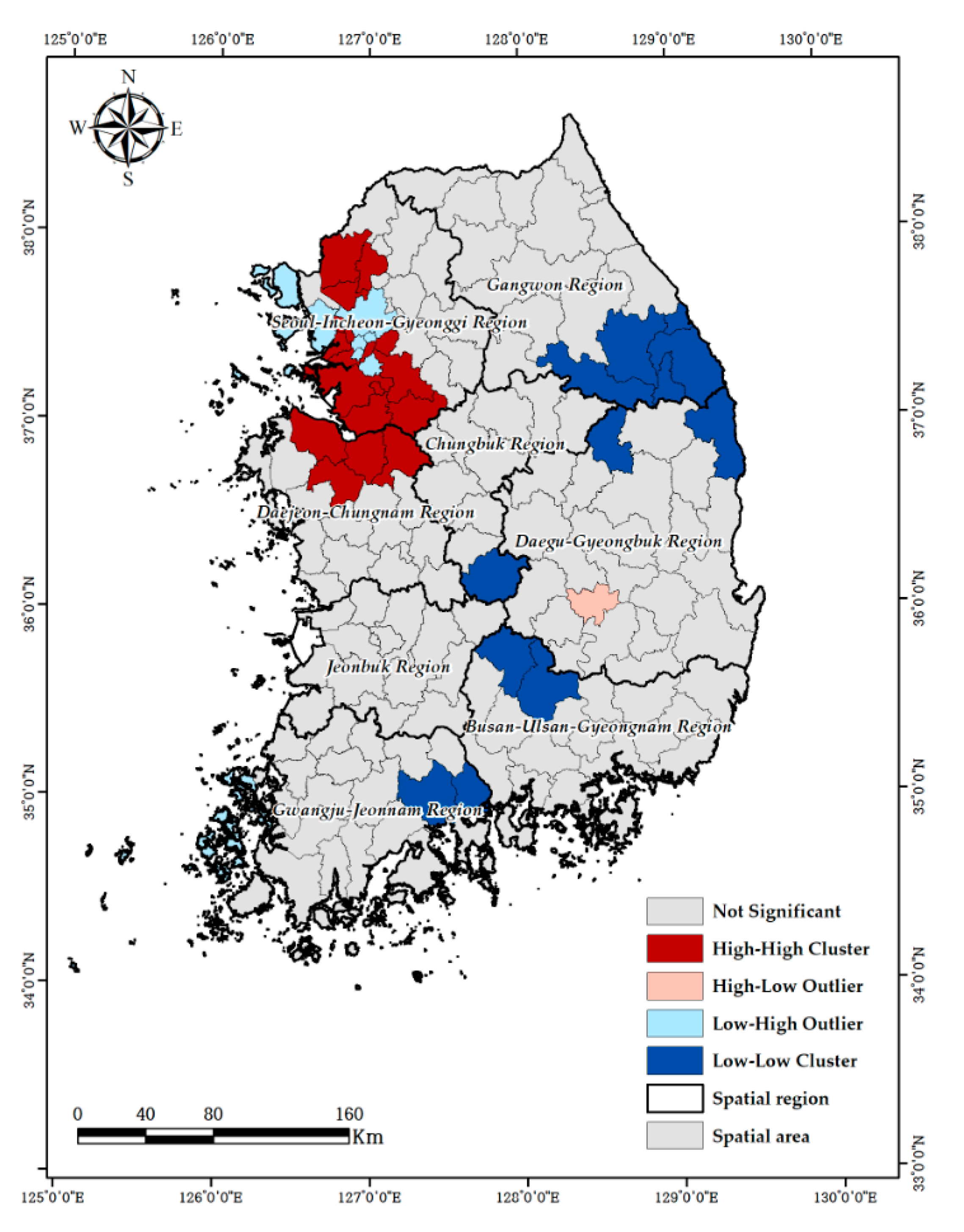
3.2. Spatial Patterns of Forest Loss

The spatial distribution characteristics of forest loss are shown in Figure 6. Forest loss showed significant positive spatial autocorrelation (global Moran’s I = 0.29, p < 0.01), indicating that forest loss was clustered. A high number of HH clusters occurred in the Seoul–Incheon–Gyeonggi region, approximately 77% of all HH clusters. Seoul-si, Incheon-si, Gimpo-si, Hwaseong-si, and Pyeongtaek-si, which are in the capital region, had many large-scale development projects (e.g., for housing, urban development, multicomplexes, free economic zones, etc.), which were either ongoing or completed in 2021. This is presumed to have led to the higher rate of forest loss in this region compared with other spatial regions. The possibility of continuous forest loss is also predicted to be high in this region [99]. Approximately 42% of clusters in the Gangwon region were LL clusters, and the mean forest loss rate was 0.6%, which was 1.2% lower than the mean forest loss rate across all spatial areas (1.8%). HL spatial outliers were mostly found close to LL clusters, whereas LH spatial outliers were mostly found close to HH clusters. The forest loss rate in the areas with HL outliers was 1.9%, which was 0.1% higher than the mean forest loss rate across all spatial areas (1.8%). This is presumably because the distribution of forest loss rate in the neighboring regions (i.e., Daegu-si, Gumi-si, Gimcheon-si, Gunwui-gun, and Seongju-gun; 0.6%) was 1.2% lower than the mean forest loss rate across all areas. Most LH spatial outliers were found in the Seoul–Incheon–Gyeonggi region, presumably due to the presence of HH clusters in the surrounding areas (Figure 6).

3.3. Assessment of Factors Impacting Forest Loss

3.3.1. Selection of Variables Related to the Factors Impacting Forest Loss

Prior to the selection of variables related to the impact factors of forest loss, multicollinearity and correlation analyses were performed for the variables. As shown in Table 5, the population and number of households showed VIFs of approximately 28 and 26, respectively; therefore, reanalysis was conducted after excluding the population. The results of the reanalysis showed that the multicollinearity was reduced to ≤10, and the remaining variables were selected as the final variables. (

Table 6. Correlation coefficients and variance inflation factors (VIFs) among variables potentially influencing forest loss. See Table 3 for variable abbreviations.

Category	Rd	Ca	Ga	Sa	P	Nh	Pm	Pe	Sm	Se	Tm	Te	VIF
Rd	1	-	-	-	-	-	-						1.3
Ca	−0.312 **	1	-	-	-	-	-	-	-	-	-	-	1.5
Ga	−0.059	0.143	1	-	-	-	-	-	-	-	-	-	1.0
Sa	0.047	0.145	−0.044	1	-	-	-	-	-	-	-	-	1.6
P	0.333 **	−0.267 **	−0.166 *	0.448 **	1	-	-	-	-	-	-	-	28.7
Nh	0.347 **	−0.328 **	−0.168 *	0.455 **	0.976 **	1	-	-	-	-	-	-	26.5
Pm	−0.039	0.093	0.025	0.089	0.011	−0.012	1	-	-	-	-	-	3.1
Pe	−0.121	0.174	0.025	0.097	−0.036	−0.067	0.812 **	1	-	-	-	-	3.2
Sm	−0.033	0.138	−0.033	0.340 **	0.206 *	0.177 *	0.058	0.049	1	-	-	-	1.8
Se	−0.171 *	0.186 *	−0.011	0.246 **	0.186 *	0.153	0.092	0.176 *	0.624 **	1	-	-	2.0
Tm	0.340 **	−0.183 *	−0.171*	0.373 **	0.811 **	0.769 **	0.049	−0.032	0.245 **	0.292 **	1	-	6.7
Te	0.351 **	−0.288 **	−0.197*	0.321 **	0.855 **	0.830 **	0.050	−0.036	0.243 **	0.278 **	0.910 **	1	8.6

* p < 0.10, ** p < 0.05.

).

3.3.2. Model Fitness Test

The fitness of each of the three models is presented in

Table 7. Model fitness test of the statistical models and machine-learning model.

Model	R2	RMSE	MAE	AICc
OLS	0.48	1.54	1.05	591.4
GWR	0.69	1.17	0.85	543.9
RF	0.69	1.17	0.88	-

. The GWR model showed better performance than the OLS model and the RF model in explaining the correlation between forest loss and its impact factors. The R2 of the GWR model was 0.69, which was 1.4-fold higher than the OLS model and equivalent to the RF model. The RMSE of the GWR model was 1.17, which was 0.37 lower than the OLS model but equivalent to the RF model. The MAE of the GWR model was 0.85, which was 0.2 and 0.03 lower than that of the OLS and RF models, respectively. The AICc of the GWR was lower than that of the OLS model by approximately 48. The GWR model was similar to the RF model with respect to R² and RMSE; however, a lower MAE meant that the GWR model most accurately explained the relationship between the variables and forest loss (Table 7).

Our results suggest that the GWR model is more suitable than the OLS model, and unlike the OLS model, it is possible to emphasize the relationship between forest loss and impact factors by deriving results according to geographical location and regional characteristics [100,101]. In addition, as with the OLS model, the RF model analyzes the relationship between forest loss and impact factors across the entire range of research areas, so it is limited to analyze the effects of regional characteristics [36]. The GWR model is considered to be the best explanation for the relationship between forest loss and impact factors.

Table 8. The influence of each variable on forest loss in the statistical (OLS and GWR) and machine-learning (RF) models. See Table 3 for variable abbreviations.

	OLS Model	GWR Model	RF Model
Rd	0.016	0.0400	0.278
Ca	0.009	0.0245	0.012
Ga	0.019	0.0009	0.025
Sa	0.008	−0.0013	0.057
Nh	0.033	0.0253	0.258
Pm	−0.000	−0.0002	0.020
Pe	−0.000	−0.0009	0.039
Sm	0.000	0.0056	0.022
Se	−0.001	−0.0042	0.046
Tm	0.000	0.0008	0.097
Te	0.023	0.0167	0.141

shows the influence of the OLS, GWR, and RF models. The influence and importance of the models reflect the quantitative degree of the effect of independent variables on forest loss in each model. In the OLS model, the variables with the highest influence (≥0.01) on forest loss were the number of households, number of tertiary industry establishments, grassland area, and road density, whereas the variables with the lowest influence (<0.001) were the number of secondary industry establishments, number of primary industry establishments, number of secondary industry employees, and number of tertiary industry employees. In the GWR model, the variables with the highest influence (≥0.01) on forest loss were road density, number of households, cropland area, and number of tertiary industry establishments, whereas the variables with the lowest influence (<0.001) were grassland area, number of primary industry employees, and number of tertiary industry employees. In the RF model, the variables with the highest influence (≥0.01) on forest loss were road density, number of households, and number of tertiary industry establishments, whereas the variables with the lowest influence (<0.03) were cropland area, grassland area, number of primary industry employees, and number of secondary industry employees. Therefore, three variables (road density, number of households, and number of tertiary industry establishments) were the most influential variables across the three models.

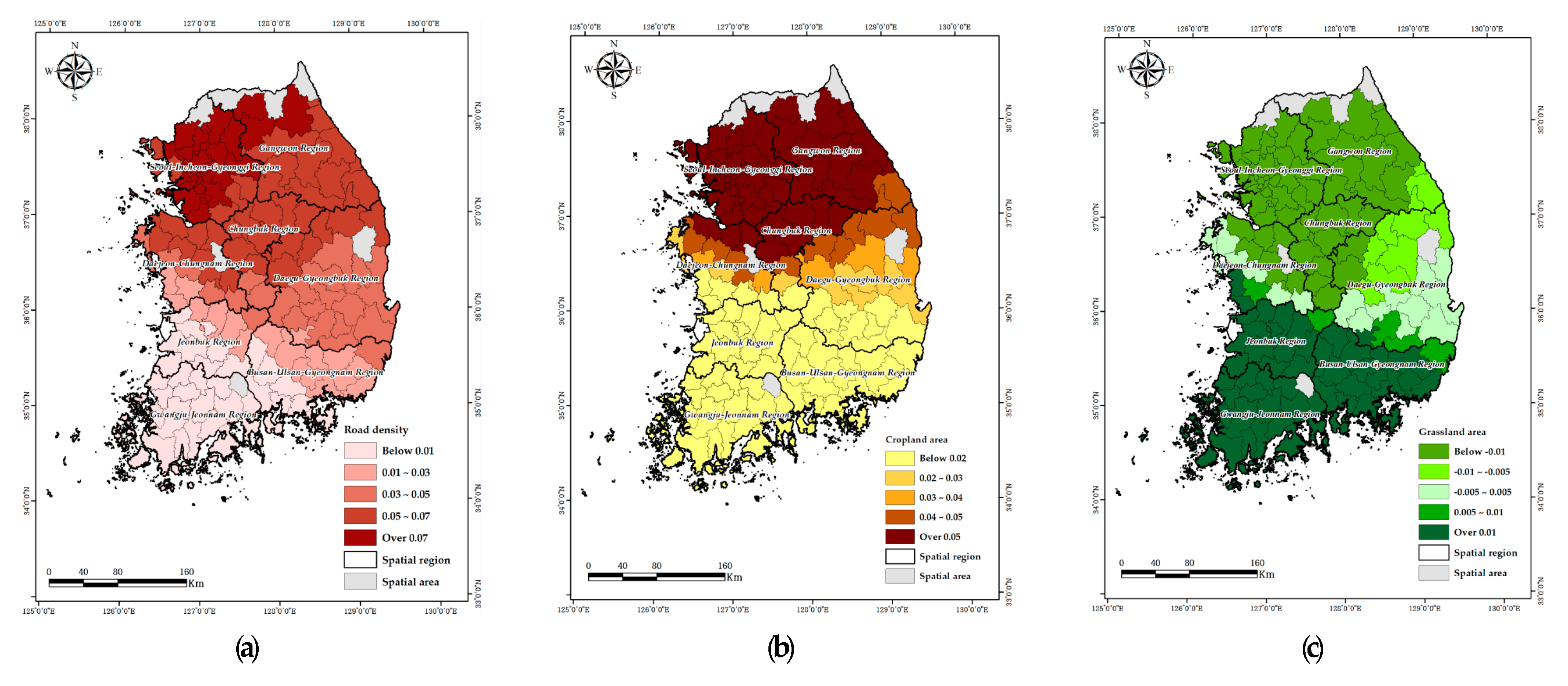
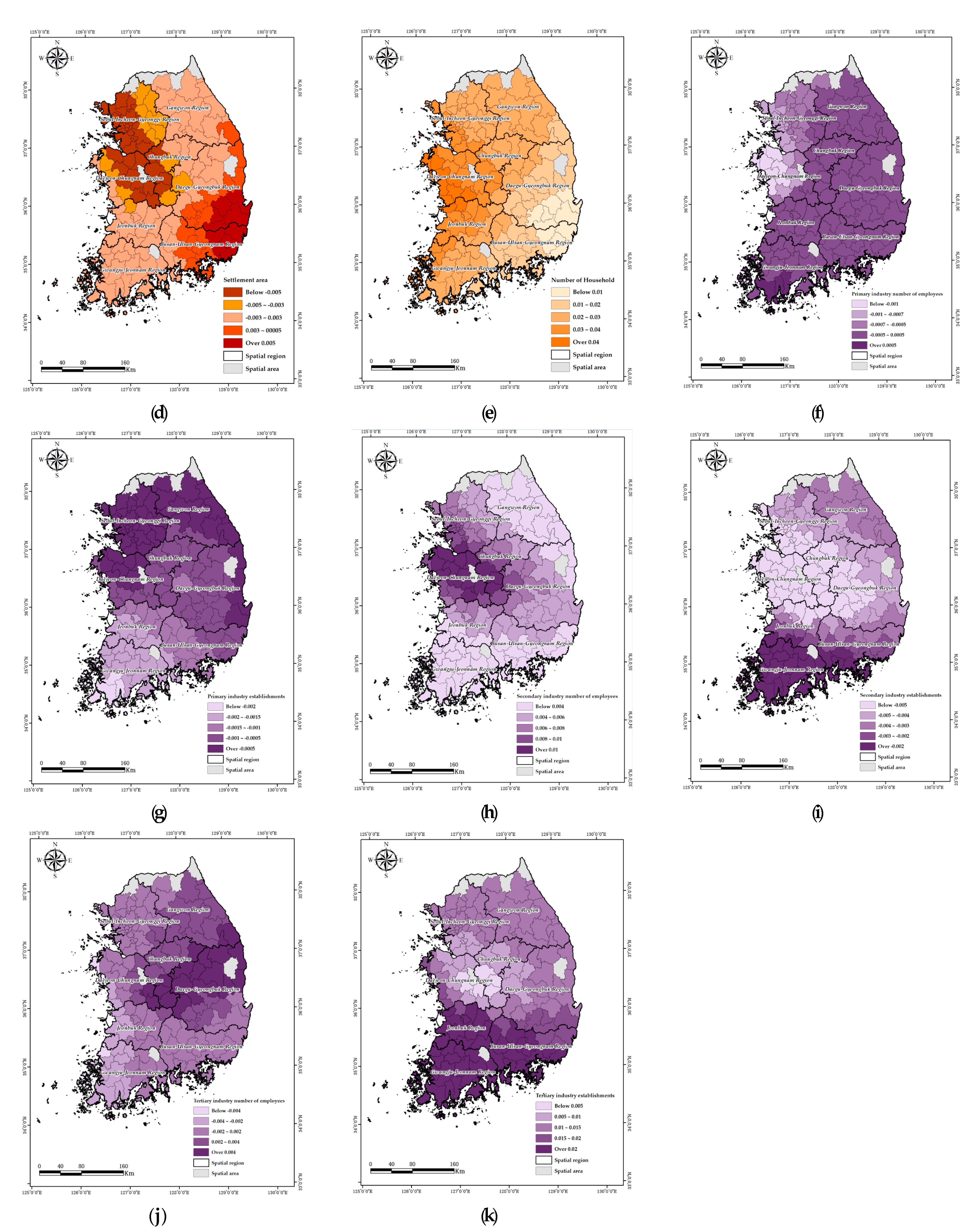
3.3.3. Assessment of Factors Impacting Forest Loss Areas in Each Spatial Region

Since the OLS model and the RF model are global models that cannot deal with spatial heterogeneity, the GWR model was used to determine the influence of factors on forest loss in each spatial region [36,90]. Figure 7 shows the results of the GWR model for each spatial area. The factors that affect the forest loss by each spatial region through the GWR model show the following characteristics.

Road density showed a major influence on forest loss in the Seoul–Incheon–Gyeonggi region, but on the contrary, a low influence in the Gwangju–Jeonnam region. The rate of increase in road density and mean rate of forest loss during 2005–2015 in the Seoul–Incheon–Gyeonggi region were 54.1% and 3.2%, respectively, both of which were the highest across the nation. The higher rate of forest loss in this region compared with other spatial regions may be attributed to the high road density in Seoul-si, Incheon-si, and Gyeonggi-do, which are categorized as the capital regions of South Korea within the Seoul–Incheon—yeonggi region, which accounted for 60% of the top 22 spatial areas with reported high road densities in 2010 [102]. The cropland area was the main cause of forest loss in the Seoul–Incheon–Gyeonggi region, but not the main cause of forest loss in the Gwangju–Jeonnam and Jeonbuk regions. The grassland area was closely related to forest loss in Gwangju–Jeonnam and Jeonbuk regions, but the relationship between forest loss and the grassland area was weak in the Seoul–Incheon–Gyeonggi and Gangwon regions. The settlement area showed a high influence on forest loss in the Busan–Ulsan–Gyeongnam region, but it showed a low influence in the Daejeon–Chungnam region. The number of households was the main factor of forest loss compared to other regions in the Daejeon–Chungnam region, whereas the number of households in the Busan–Ulsan–Gyeongnam region was not enough to factor for forest loss. Of all the metropolitan cities and provinces, Daejeon-si and Chungcheongnam-do, which belong to the Daejeon–Chungnam region, had the highest rate of increase in the number of households during 2000–2010, followed by Gyeonggi-do. This is presumed to be the reason for the high rate of forest loss in the Daejeon–Chungnam region [103].

Regarding the number of industry employees and establishments, the number of primary industry employees had a high positive effect on forest loss in the Gwangju–Jeonnam region but a negative effect in certain spatial areas in the Daejeon–Chungnam region. The number of primary industry establishments did not have much effect on the forest loss in the Gwangju–Jeonnam region. The number of secondary industry employees was the main cause of forest loss in the Daejeon–Chungnam region, but not in Gwangju–Jeonnam region. In the Chungcheongnam-do area of the Daejeon–Chungnam region, the manufacturing industry contributed to 46.9% of the gross domestic regional production in 2006, which was higher than the national average (28.2%) [104]. Therefore, it is presumed that the increase in secondary industry employees had an impact on forest loss. The number of secondary industry establishments showed a high influence on forest loss in certain spatial areas of the Gwangju–Jeonnam region, but a low influence in the Daejeon–Chungnam region. The number of tertiary industry employees was analyzed as the main factor causing forest loss in the Daegu–Gyeongbuk region, but the influence was relatively insufficient in the Gwangju–Jeonnam region. The number of tertiary industry establishments had a high influence on forest loss in the Gwangju–Jeonnam region, but a low influence in the Daejeon–Chungnam area. Mo and Lee [105] reported that in 2015, Gwangju-si in the Gwangju–Jeonnam region specialized in tertiary industries, with a high number of wholesale, retail, accommodation, food service, banking, insurance, real estate, and lease service establishments, among other tertiary industries. This is thought to have resulted in the high positive effect of tertiary industry establishments in the Gwangju–Jeonnam region. The effects of variables on forest loss differed among the spatial regions. For example, in the Seoul–Incheon–Gyeonggi region, in which there was a higher rate of forest loss, road density and number of households had a strong effect on forest loss. Conversely, in the Daejeon–Chungnam region, the number of secondary industry employees had a strong effect on forest loss (Figure 7).

The effect of these factors on forest loss is due to urbanization [106,107]. Urbanization causes forest loss by generating high demand for residential facilities and infrastructure facilities in neighboring areas, especially in the development area, as the population and the number of households increase beyond simple regional development [108,109]. This is consistent with the results of Chen et al. that forest loss occurred due to urban development including the increase of roads and residential areas [110]. Urbanization and development are likely to continue in the future, so it is necessary to prepare measures to maintain the balance of forest conservation and forest loss between urbanization and regional development.

On the other hand, the causes of forest loss are different according to the region, as in our research [98]. In developing countries, rapid agricultural expansion and excessive use of forest resources are the main causes of forest loss, resulting in forest loss due to food demand problems and agricultural investment [111,112]. For example, in Malawi, the expansion of agricultural land such as corn farm expansion, tobacco cultivation, and brick production is one of the main causes of forest loss [113]. Myanmar’s expansion of agricultural land following rapid agricultural investment and expansion of the city is among the main causes of forest loss. Then, the factors for forest loss differ according to the region [69,114]. In addition, in countries such as Bhutan, Laos, Nepal, Sri Lanka, and Vietnam, topographical conditions (altitude, slope) and biophysical requirements such as temperature and precipitation were also among the main factors in the loss of forest area [115]. In the United States, factories, houses, and roads have had a great impact on forest loss, which is also the difference in accessibility, lifestyle, and institution [116]. As the relationship between forest loss and impact factors differs by country and region, studies are being conducted on various regions. Mwangi et al. analyzed the relationship between forest loss and impact factors on randomly selected sites using land coverage maps in the Central Region and analyzed that topographic factors (altitude, slope), distance from roads and distance from rivers are the main causes of forest loss [117]. This study analyzed the influence of topographic factors and forest loss, unlike our research, which showed that the closer the distance from the road and the closer the river, the easier the transportation, resulting in forest loss. Santos et al. [118] analyzed the relationship between forest loss and impact factors in the Amazon region of Brazil and confirmed that the rapid expansion of roads, ranches, and agricultural products affected the loss of forest. This means that the increase in roads increases accessibility, which is believed to have promoted the change of forest into cropland and pasture [9,118]. In addition, Mas and Cuevas analyzed the forest loss status based on the municipality, and then analyzed the effect on forest loss using the GWR model, and confirmed that the same factors could have different effects depending on the region. On the other hand, the forest loss and its impact factors were also conducted through preceding research. Geist and Lambin analyzed the causes of forest loss by dividing them into proximate causes and underlying driving forces through preceding research review and analyzed that the impact of the forest loss was on agricultural expansion, the use of timber and infrastructure expansion, economic and commercialization, and institutional and demographic factors [23]. In addition, Armenteras et al. [119] analyzed the previous studies conducted on Latin American countries to analyze the factors affecting forest loss and its impacts and confirmed that access to markets and agricultural and forest activities had a major impact on forest loss. As the factors of forest loss and its impact differ by region, studies are being conducted on various continents and regions. Forests are decreased by the above-mentioned factors, and this is affected by regional socioeconomic factors, institutional factors, and topographic factors, so they should be analyzed considering these factors. Therefore, causes of forest loss are different in each region, which is judged to be due to the differences in socioeconomic, biophysical characteristics, policies, and institutions of each region [19,22,100,120].

3.4. Limitations of the Study

Meanwhile, this study has certain limitations. First, we analyzed forest loss and factors at the administrative district level. However, spatial analyses using grids or micropolygon units can provide more details regarding the effects of factors on forests [121,122]. Another limitation was the selection of factors influencing forest loss. We did not include several variables that have recently been found to affect forest loss in South Korea, such as altitude, slope, and photovoltaic solar plants [123,124]. The lower the altitude and slope, the easier the accessibility, so the agricultural forest clearing is advantageous, and the forest loss appears. However, the altitude and slope were not used in this study because securing the time-series data was limited compared to other forest loss factors [123]. In the case of the photovoltaic solar plants, according to Mori and Tabata [125], there are benefits such as mitigation of climate change and economic benefits, but it can cause biodiversity due to forest loss, loss of carbon sinks, and risk of landslides. However, this study did not utilize it due to the limitation of securing time-series data. Therefore, future studies need to discuss the effects of geographical factors (high altitude, slope), photovoltaic solar plants, etc., on forest loss and the problems that can be caused.

Therefore, considerable efforts are required to more clearly predict factors affecting forest loss by including suitable factors in each spatial area. Results of this study may contribute to the development of policies for reducing forest loss and provide valuable data on the correlation between forest loss and the factors impacting this process. Further studies are needed to address the limitations of this study to enhance the applicability of the results.

4. Conclusions

We analyzed the spatial distribution of forest loss in Korea and the factors affecting forest loss. The results of this study showed that forest loss occurred in large quantities mainly in the Seoul–Incheon–Gyeonggi region and was 1.8 times higher than the average forest loss in South Korea. As a result of Moran’s I analysis, HH clusters occurred mainly in the Seoul–Incheon–Gyeonggi region, which shows that forest loss occurred mainly in the Seoul–Incheon–Gyeonggi region. The forest loss and its impact factors were analyzed using OLS, GWR, and RF models. The GWR model had a 1.4-fold higher R² than the OLS model, and the AICc was about 48 less. In addition, the MAE was lower than the RF model, showing the highest model suitability. This means that the GWR model can perform a better regional approach to forest loss and its impact compared to the OLS model and the RF model, and it suggests that the GWR model is easy to analyze according to regional differences. The most frequent forest loss in the Seoul–Incheon–Gyeonggi region was found to have a strong impact on road density and number of households. This is due to the progress of road construction and infrastructure installation as urbanization progresses mainly in the Seoul–Incheon–Gyeonggi region between 2005 and 2015. In particular, according to Liu et al. [126], infrastructure construction and economic growth are the main causes of forest loss, and forest loss appears to have occurred as developments have progressed around the region.

On the other hand, since forest loss varies according to regional characteristics, research needs to be conducted based on background knowledge of the region [101]. Therefore, the analysis of factors affecting forest loss should be carried out in consideration of the situation of each country and region as in the previous studies, and both biophysical and socioeconomic factors should be considered as much as possible. The GWR model is useful for quantitative analysis of forest loss factors by region, and it is expected to be useful for policy design and evaluation of forest loss by using it together with qualitative analysis. In addition, if we analyze the changes in the forest loss and its impact factors, which were mentioned earlier, it will be useful data for policy setting. Therefore, in future studies, it is necessary to analyze the changes and causes of forest loss over time using the local Moran’s I, time-series and hotspot analysis, and GWR model. Clearing the factors affecting forest loss will be useful for establishing forest management plans and improving forest protection systems.

References

1. Food and Agriculture Organization of the United Nations (FAO). Global Forest Resources Assessment 2020; Main Report; FAO: Rome, Italy, 2020. [Google Scholar]
2. Prevedello, J.A.; Winck, G.R.; Weber, M.M.; Nichols, E.; Sinervo, B. Impacts of Forestation and Deforestation on Local Temperature Across the Globe. PLoS ONE 2019, 14, e0213368. [Google Scholar] [CrossRef] [Green Version]
3. Intergovernmental Panel on Climate Change (IPCC). Climate Change 2014: Contribution of Working Groups I, II and III to the Fifth Assessment Report of the Intergovernmental Panel on Climate Change; Synthesis Report; IPCC: Geneva, Switzerland, 2014. [Google Scholar]
4. Giesekam, J.; Tingley, D.D.; Cotton, I. Aligning carbon targets for construction with (inter) national climate change mitigation commitments. Energy Build. 2018, 165, 106–117. [Google Scholar] [CrossRef]
5. Tyukavina, A.; Hansen, M.C.; Potapov, P.; Parker, D.; Okpa, C.; Stehman, S.V.; Kommareddy, I.; Turubanova, S. Congo Basin forest loss dominated by increasing smallholder clearing. Sci. Adv. 2018, 4, eaat2993. [Google Scholar] [CrossRef] [Green Version]
6. Cohn, A.S.; Bhattarai, N.; Campolo, J.; Crompton, O.; Dralle, D.; Duncan, J.; Thompson, S. Forest loss in Brazil increases maximum temperatures within 50 km. Environ. Res. Lett. 2019, 14, 084047. [Google Scholar] [CrossRef] [Green Version]
7. Zhu, Z.; Zhu, X. Study on Spatiotemporal Characteristic and Mechanism of Forest Loss in Urban Agglomeration in the Middle Reaches of the Yangtze River. Forests 2021, 12, 1242. [Google Scholar] [CrossRef]
8. Zheng, Z.; Ma, T.; Roberts, P.; Li, Z.; Yue, Y.; Peng Huang, K.; Han, Z.; Wan, Q.; Zhang, Y.; Zhang, X.; et al. Anthropogenic impacts on Late Holocene land-cover change and floristic biodiversity loss in tropical southeastern Asia. Proc. Natl. Acad. Sci. USA 2021, 118, e2022210118. [Google Scholar] [CrossRef]
9. Laurance, W.F.; Sayer, J.; Cassman, K.G. Agricultural expansion and its impacts on tropical nature. Trends Ecol. Evol. 2014, 29, 107–116. [Google Scholar] [CrossRef] [PubMed]
10. Nobre, C.A.; Sampaio, G.; Borma, L.S.; Castilla-Rubio, J.C.; Silva, J.S.; Cardoso, M. Land-use and climate change risks in the Amazon and the need of a novel sustainable development paradigm. Proc. Natl. Acad. Sci. USA 2016, 113, 10759–10768. [Google Scholar] [CrossRef] [PubMed] [Green Version]
11. Korea Forest Service. Forest Basic Statistics; Korea Forest Service: Daejeon, Korea, 2020.
12. Korea Forest Service. Statistical Yearbook of Forestry; Korea Forest Service: Daejeon, Korea, 2020.
13. Kim, S.B.; Hwang, S.T. A Study on Extraction and Classification of Unlawful Forest Land Diversion by Using GIS. Korean Public Adm. Q. 2015, 27, 513–542. [Google Scholar]
14. Aide, T.M.; Clark, M.L.; Grau, H.R.; López-Carr, D.; Levy, M.A.; Redo, D.; Andrade-Núñez, M.J.; Muñiz, M. Deforestation and Reforestation of Latin America and the Caribbean (2001–2010). Biotropica 2012, 45, 262–271. [Google Scholar] [CrossRef]
15. Dlamini, W.M. Analysis of Deforestation Patterns and Drivers in Swaziland using Efficient Bayesian Multivariate Classifiers. Model. Earth Syst. Environ. 2016, 2, 1–14. [Google Scholar] [CrossRef]
16. Mayfield, H. Making the Most of Machine Learning and Freely Available Datasets: A Deforestation Case Study. Ph.D. Thesis, The University of Queensland, Queensland, Australia, 2015. [Google Scholar]
17. Verburg, R.; Filho, S.R.; Lindoso, D.; Debortoli, N.; Litre, G.; Bursztyn, M. The Impact of Commodity Price and Conservation Policy Scenarios on Deforestation and Agricultural Land Use in a Frontier Area within the Amazon. Land Use Policy 2014, 37, 14–26. [Google Scholar] [CrossRef]
18. Damnyag, L.; Saastamoinen, O.; Blay, D.; Dwomoh, F.K.; Anglaaere, L.C.; Pappinen, A. Sustaining Protected Areas: Identifying and Controlling Deforestation and Forest Degradation Drivers in the Ankasa Conservation Area, Ghana. Biol. Conserv. 2013, 165, 86–94. [Google Scholar] [CrossRef]
19. Scullion, J.J.; Vogt, K.A.; Drahota, B.; Winkler-Schor, S.; Lyons, M. Conserving the Last Great Forests: A Meta-analysis Review of the Drivers of Intact Forest Loss and the Strategies and Policies to Save Them. Front. For. Glob. Change. 2019, 2, 62. [Google Scholar] [CrossRef]
20. Echeverria, C.; Coomes, D.A.; Hall, M.; Newton, A.C. Spatially explicit models to analyze forest loss and fragmentation between 1976 and 2020 in southern Chile. Ecol. Modell. 2008, 212, 439–449. [Google Scholar] [CrossRef]
21. Gayen, A.; Saha, S. Deforestation probable area predicted by logistic regression in Pathro river basin: A tributary of Ajay River. Spatial. Inf. Res. 2018, 26, 1–9. [Google Scholar] [CrossRef]
22. Sharma, P.; Thapa, R.B.; Matin, M.A. Examining Forest cover change and deforestation drivers in Taunggyi District, Shan State, Myanmar. Environ. Dev. Sustain. 2020, 22, 5521–5538. [Google Scholar] [CrossRef] [Green Version]
23. Geist, H.J.; Lambin, E.F. Proximate Causes and Underlying Driving Forces of Tropical Deforestation: Tropical Forests are Disappearing as the Result of Many Pressures, both Local and Regional, Acting in Various Combinations in Different Geographical Locations. Bioscience 2002, 52, 143–150. [Google Scholar] [CrossRef]
24. Brondizio, E.S.; Moran, E.F. Level-Dependent Deforestation Trajectories in the Brazilian Amazon from 1970 to 2001. Popul. Environ. 2012, 34, 69–85. [Google Scholar] [CrossRef]
25. Cochard, R.; Ngo, D.T.; Waeber, P.O.; Kull, C.A. Extent and Causes of Forest Cover Changes in Vietnam’s Provinces 1993–2013: A Review and Analysis of Official Data. Environ. Rev. 2017, 25, 199–217. [Google Scholar] [CrossRef] [Green Version]
26. Jusys, T. Fundamental Causes and Spatial Heterogeneity of Deforestation in Legal Amazon. Appl. Geogr. 2016, 75, 188–199. [Google Scholar] [CrossRef]
27. Trigueiro, W.R.; Nabout, J.C.; Tessarolo, G. Uncovering the Spatial Variability of Recent Deforestation Drivers in the Brazilian Cerrado. J. Environ. Manag. 2020, 275, 111243. [Google Scholar] [CrossRef] [PubMed]
28. Anselin, L. Local Indicators of Spatial Association-LISA. Geogr. Anal. 1995, 27, 93–115. [Google Scholar] [CrossRef]
29. Harris, N.L.; Goldman, E.; Gabris, C.; Nordling, J.; Minnemeyer, S.; Ansari, S.; Lippmann, M.; Bennett, L.; Raad, M.; Hansen, M.; et al. Using Spatial Statistics to Identify Emerging Hot Spots of Forest Loss. Environ. Res. Lett. 2017, 12, 024012. [Google Scholar] [CrossRef]
30. Cushman, S.A.; Macdonald, E.A.; Landguth, E.L.; Malhi, Y.; Macdonald, D.W. Multiple-scale Prediction of Forest Loss Risk Across Borneo. Landsc. Ecol. 2017, 32, 1581–1598. [Google Scholar] [CrossRef] [Green Version]
31. Uvsh, D.; Gehlbach, S.; Potapov, P.V.; Munteanu, C.; Bragina, E.V.; Radeloff, V.C. Correlates of Forest-cover Change in European Russia, 1989–2012. Land Use Policy. 2020, 96, 104648. [Google Scholar] [CrossRef]
32. Mohamed, M.A. An Assessment of Forest Cover Change and Its Driving Forces in the Syrian Coastal Region during a Period of Conflict, 2010 to 2020. Land 2021, 10, 191. [Google Scholar] [CrossRef]
33. Clement, F.; Orange, D.; Williams, M.; Mulley, C.; Epprecht, M. Drivers of Afforestation in Northern Vietnam: Assessing Local Variations using Geographically Weighted Regression. Appl. Geogr. 2009, 29, 561–576. [Google Scholar] [CrossRef]
34. Chen, L.; Ren, C.; Zhang, B.; Wang, Z.; Xi, Y. Estimation of forest above-ground biomass by geographically weighted regression and machine learning with sentinel imagery. Forests 2018, 9, 582. [Google Scholar] [CrossRef] [Green Version]
35. Breiman, L. Random forests. Mach. Learn. 2001, 45, 5–32. [Google Scholar] [CrossRef] [Green Version]
36. Georganos, S.; Grippa, T.; Niang Gadiaga, A.; Linard, C.; Lennert, M.; Vanhuysse, S.; Mboga, N.; Wolff, E.; Kalogirou, S. Geographical Random Forests: A Spatial Extension of the Random Forest Algorithm to Address Spatial Heterogeneity in Remote Sensing and Population Modelling. Geocarto. Int. 2021, 36, 121–136. [Google Scholar] [CrossRef] [Green Version]
37. Zamani Joharestani, M.; Cao, C.; Ni, X.; Bashir, B.; Talebiesfandarani, S. PM2. 5 prediction based on random forest, XGBoost, and deep learning using multisource remote sensing data. Atmosphere 2019, 10, 373. [Google Scholar] [CrossRef] [Green Version]
38. Kim, C.K.; Jeong, S.Y.; Kwon, S.D.; Kim, W.K. A Study on the Possibility for the Introduction of Forest Land Reverse Mortgage System. J. KIFR 2014, 18, 39–47. [Google Scholar]
39. Park, I.S.; Kim, E.J.; Hong, S.O.; Kang, S.H. A Study on Factors Related with Regional Occurrence of Cardiac Arrest Using Geographically Weighted Regression. Health Soc. Welf. Rev. 2013, 33, 237–257. [Google Scholar]
40. Sung, J.H.; Chae, G.S. Analysis of Economic Impact in Drought: Focusing on Rice production. JRD 2018, 41, 1–23. [Google Scholar]
41. Lee, C.W.; Yoo, D.G. Evaluation of Drought Resilience Reflecting Regional Characteristics: Focused on 160 Local Governments in Korea. Water 2021, 13, 1873. [Google Scholar] [CrossRef]
42. Korea Forest Service. Forest Basic Statistics; Korea Forest Service: Daejeon, Korea, 2005.
43. Korea Forest Service. Forest Basic Statistics; Korea Forest Service: Daejeon, Korea, 2015.
44. Lee, S.J.; Yim, J.S.; Son, Y.M.; Kim, R.H. Recalculation of Forest Growing Stock for National Greenhouse Gas Inventory. J. Climate. Change. Res. 2016, 7, 485–492. [Google Scholar] [CrossRef]
45. Park, J.M.; Lee, J.S.; Lee, H.S.; Park, J.W. Study on Timber Yield Regulation Method using Probability Density Function. J. Korean Soc. For. Sci. 2020, 109, 504–511. [Google Scholar]
46. Ministry of Land, Infrastructure and Transport. Cadastral Statistic Annual Report; Ministry of Land, Infrastructure and Transport: Sejong, Korea, 2005.
47. Ministry of Land, Infrastructure and Transport. Cadastral Statistic Annual Report; Ministry of Land, Infrastructure and Transport: Sejong, Korea, 2015.
48. Statistics Korea. Agricultural Area Survey; Statistics Korea: Daejeon, Korea, 2005.
49. Statistics Korea. Agricultural Area Survey; Statistics Korea: Daejeon, Korea, 2015.
50. Statistics Korea. Agriculture, Forestry and Fishery Survey; Statistics Korea: Daejeon, Korea, 2005.
51. Statistics Korea. Agriculture, Forestry and Fishery Survey; Statistics Korea: Daejeon, Korea, 2015.
52. Ministry of Employment and Labor. Survey of Establishments; Ministry of Employment and Labor: Sejong, Korea, 2005.
53. Ministry of Employment and Labor. Survey of Establishments; Ministry of Employment and Labor: Sejong, Korea, 2015.
54. Park, E.B.; Song, C.H.; Ham, B.Y.; Kim, J.W.; Lee, J.Y.; Choi, S.E.; Lee, W.K. Comparison of Sampling and Wall-to-Wall Methodologies for Reporting the GHG Inventory of the LULUCF Sector in Korea. J. Climate Change Res. 2018, 9, 385–398. [Google Scholar] [CrossRef]
55. Lee, H.M.; Goh, J.T. Factors Influencing Cultivated Area Decisions of the Rural Area in the Fringe of Small and Medium Sizes City. J. Korean Soc. Rural Plann. 2015, 21, 1–10. [Google Scholar] [CrossRef]
56. Sim, S.Y.; Lee, K.W.; Kim, M.G.; Park, J.Y. The Case of Utilization on Regional Agricultural Statistics information. Korea Rural Econ. Inst. 2019, 1–151. [Google Scholar]
57. Lee, J.M. Analysis of the Status of Agricultural Communities and Location Quotient (LQ) using Regional Survey Data in 2015 Census of Agriculture, Forestry, and Fisheries. J. Korean Soc. Rural Plan. 2020, 26, 83–93. [Google Scholar] [CrossRef]
58. Kim, S.Y.; Park, H.; Koo, H.M.; Ryoo, D.K. The Effects of the Port Logistics Industry on Port City’s Economy. J. Navig. Port. Res. 2015, 39, 267–275. [Google Scholar] [CrossRef] [Green Version]
59. Lee, Y.G.; Jung, C.G.; Kim, W.J.; Kim, S.J. Analysis of National Stream Drying Phenomena using DrySAT-WFT Model: Focusing on Inflow of Dam and Weir Watersheds in 5 River Basins. J. KAGIS 2020, 23, 53–69. [Google Scholar]
60. Dai, W.; Li, Y.; Fu, W.; Jiang, P.; Zhao, K.; Li, Y.; Penttinen, P. Spatial Variability of Soil nutrients in Forest Areas: A Case Study from Subtropical China. J. Plant. Nutr. Soil. Sci. 2018, 181, 827–835. [Google Scholar] [CrossRef]
61. Pan, P.; Sun, Y.; Ouyang, X.; Zang, H.; Rao, J.; Ning, J. Factors Affecting Spatial Variation in Vegetation Carbon Density in Pinus massoniana Lamb. Forest in Subtropical China. Forests 2019, 10, 880. [Google Scholar] [CrossRef] [Green Version]
62. Ma, W.; Chen, J.; Chen, P. Illegal Activities Hotspot Analysis Based on GIS methods. In Proceedings of the 2nd IEEE International Conference on Emergency Management and Management Sciences, Beijing, China, 8–10 August 2011; Institute of Electrical and Electronics Engineers: Piscataway, NJ, USA, 2011; pp. 270–273. [Google Scholar]
63. Sánchez-Martín, J.M.; Rengifo-Gallego, J.I.; Blas-Morato, R. Hot Spot Analysis Versus Cluster and Outlier Analysis: An Enquiry into the Grouping of Rural Accommodation in Extremadura (Spain). ISPRS Int. J. GeoInf. 2019, 8, 176. [Google Scholar] [CrossRef] [Green Version]
64. Islam, A.; Sayeed, M.A.; Rahman, M.K.; Ferdous, J.; Islam, S.; Hassan, M.M. Geospatial Dynamics of COVID-19 Clusters and Hospots in Bangladesh. Transbound Emerg. Dis. 2021, 68, 3643–3657. [Google Scholar] [CrossRef] [PubMed]
65. Kim, S.M.; Choi, Y. Assessment of Lead (Pb) and Zinc (Zn) Contamination in Beach Sands by Hot Spot Analysis. J. Coast. Res. 2019, 91, 321–325. [Google Scholar] [CrossRef]
66. Zhang, C.; Luo, L.; Xu, W.; Ledwith, V. Use of Local Moran’s I and GIS to Identify Pollution Hotspots of Pb in Urban Soils of Galway, Ireland. Sci. Total. Environ. 2008, 398, 212–221. [Google Scholar] [CrossRef]
67. Dilig, I.J.A.; San Juan, W.I.M. Geostatistical and Cluster Analysis of Earthquakes in the Philippines. Int. Arch. Photogramm. Remote. Sens. Spat. Inf. Sci. 2019, 42, 185–192. [Google Scholar] [CrossRef] [Green Version]
68. Mena, C.F.; Bilsborrow, R.E.; McClain, M.E. Socioeconomic Drivers of Deforestation in the Northern Ecuadorian Amazon. Environ. Manag. 2006, 37, 802–815. [Google Scholar] [CrossRef]
69. Ngwira, S.; Watanabe, T. An Analysis of the Causes of Deforestation in Malawi: A Case of Mwazisi. Land 2019, 8, 48. [Google Scholar] [CrossRef] [Green Version]
70. Walker, N.F.; Patel, S.A.; Kalif, K.A. From Amazon Pasture to the High Street: Deforestation and the Brazilian Cattle Product Supply Chain. Trop. Conserv. Sci. 2013, 6, 446–467. [Google Scholar] [CrossRef] [Green Version]
71. Jayathilake, H.M.; Prescott, G.W.; Carrasco, L.R.; Rao, M.; Symes, W.S. Drivers of Deforestation and Degradation for 28 tropical Conservation Landscapes. AMBIO 2021, 50, 215–228. [Google Scholar] [CrossRef] [PubMed]
72. Godoy, R.; Franks, J.R.; Wilkie, D.; Alvarado, M.; Gray-Molina, G.; Roca, R.; Escóbar, J.; Cardenas, M. The Effects of Economic Development on Neotropical Deforestation: Household and Village evidence from Amerindians in Bolivia; Development Discussion Papers; Harvard Institute for International Development: Cambridge, MA, USA, 1996. [Google Scholar]
73. Biswas, S.; Swanson, M.E.; Vacik, H. Natural Resources Depletion in Hill Areas of Bangladesh: A Review. J. Math. Sci. 2012, 9, 147–156. [Google Scholar] [CrossRef]
74. Lata, K.; Misra, A.K.; Shukla, J.B. Modeling the Effect of Deforestation Caused by Human Population Pressure on Wildlife Species. Nonlinear. Anal. Modell. Control. 2018, 23, 303–320. [Google Scholar] [CrossRef]
75. Fisher, A.G. Clash of Progress and Security; Macmillan and Co. Ltd.: London, UK, 1935. [Google Scholar]
76. Freund, R.J.; Wilson, W.J.; Sa, P. Regression: Analysis; Elsevier: Amsterdam, The Netherlands, 2006. [Google Scholar]
77. Tu, J. Spatial Variations in the Relationships Between Land Use and Water Quality across an Urbanization Gradient in the Watersheds of Northern Georgia, USA. Environ. Manag. 2013, 51, 1–17. [Google Scholar] [CrossRef]
78. Foody, G.M. Geographical Weighting as a Further Refinement to Regression Modelling: An Example Focused on the NDVI–Rainfall Relationship. Remote Sens. Environ. 2003, 88, 283–293. [Google Scholar] [CrossRef]
79. Xie, W.; Yi, S.; Leng, C.A. Study to Compare Three Different Spatial Downscaling Algorithms of Annual TRMM 3B43 Precipitation. In Proceedings of the 26th International. Conference on Geoinformatics, Kunming, China, 28–30 June 2018; Institute of Electrical and Electronics Engineers: Piscataway, NJ, USA, 2018; pp. 1–6. [Google Scholar]
80. Wang, Q.; Ni, J.; Tenhunen, J. Application of a Geographically-weighted Regression Analysis to Estimate Net Primary Production of Chinese Forest Ecosystems. Glob. Ecol. Biogeogr. 2005, 14, 379–393. [Google Scholar] [CrossRef]
81. Wang, J.; Wang, S.; Li, S. Examining the Spatially Varying Effects of Factors on PM2. 5 Concentrations in Chinese Cities using Geographically Weighted Regression Modeling. Environ. Pollut. 2019, 248, 792–803. [Google Scholar] [CrossRef]
82. Kumari, M.; Singh, C.K.; Bakimchandra, O.; Basistha, A. Geographically Weighted Regression Based Quantification of Rainfall–Topography Relationship and Rainfall Gradient in Central Himalayas. Int. J. Climatol. 2017, 37, 1299–1309. [Google Scholar] [CrossRef]
83. Tu, J.; Xia, Z.G. Examining spatially varying relationships between land use and water quality using geographically weighted regression I: Model design and evaluation. Sci. Total. Environ. 2008, 407, 358–378. [Google Scholar] [CrossRef] [PubMed]
84. Shah, S.H.; Angel, Y.; Houborg, R.; Ali, S.; McCabe, M.F. A Random Forest Machine Learning Approach for the Retrieval of Leaf Chlorophyll Content in Wheat. Remote. Sens. 2019, 11, 920. [Google Scholar] [CrossRef] [Green Version]
85. Abdulkareem, N.M.; Abdulazeez, A.M. Machine Learning Classification Based on Radom Forest Algorithm: A Review. Int. J. Sci. Bus. 2021, 5, 128–142. [Google Scholar]
86. Bunn, C.; Talsma, T.; Läderach, P.; Castro, F. Climate Change Impacts on Indonesian Cocoa Areas. In Cocoa Climate Suitability Indonesia 2017 CIAT 50 and Mondelez International. Available online: https://www.cocoalife.org/progress/climate-change-impacts-on-indonesian-cocoa-areas-report (accessed on 3 November 2021).
87. Liu, Y.; Wu, H. Prediction of Road Traffic Congestion Based on Random Forest. In Proceedings of the 10th International Symposium on Computational Intelligence and Design (ISCID), Hangzhou, China, 9–10 December 2017; Institute of Electrical and Electronics Engineers: Piscataway, NJ, USA, 2017; Volume 2, pp. 361–364. [Google Scholar]
88. Krishnamurthy, N.; Maddali, S.; Hawk, J.A.; Romanov, V.N. 9Cr steel visualization and predictive modeling. Comput. Mater. Sci. 2019, 168, 268–279. [Google Scholar] [CrossRef]
89. Song, X.; Long, Y.; Zhang, L.; Rossiter, D.G.; Liu, F.; Jiang, W. Spatial Accuracy Evaluation for Mobile Phone Location Data with Consideration of Geographical Context. IEEE Access. 2020, 8, 221176–221190. [Google Scholar] [CrossRef]
90. Koh, E.H.; Lee, E.; Lee, K.K. Application of Geographically Weighted Regression Models to Predict Spatial Characteristics of Nitrate Contamination: Implications for an Effective Groundwater Management Strategy. J. Environ. Manag. 2020, 268, 110646. [Google Scholar] [CrossRef]
91. Chen, F.W.; Liu, C.W. Estimation of the Spatial Rainfall Distribution using Inverse Distance Weighting (IDW) in the Middle of Taiwan. Paddy Water Environ. 2012, 10, 209–222. [Google Scholar] [CrossRef]
92. Willmott, C.J. Some Comments on the Evaluation of Model Performance. Bull. Am. Meteor. Soc. 1982, 63, 1309–1313. [Google Scholar] [CrossRef] [Green Version]
93. Khodadoust Siuki, S.; Saghafian, B.; Moazami, S. Comprehensive Evaluation of 3-hourly TRMM and Half-hourly GPM-IMERG Satellite Precipitation Products. Int. J. Remote Sens. 2017, 38, 558–571. [Google Scholar] [CrossRef]
94. Burnham, K.P.; Anderson, D.R. Multimodel Inference: Understanding AIC and BIC in Model Selection. Soc. Methods Res. 2004, 33, 261–304. [Google Scholar] [CrossRef]
95. Nashwari, I.P.; Rustiadi, E.; Siregar, H.; Juanda, B. Geographically Weighted Regression Model for Poverty Analysis in Jambi Province. Indones. J. Geogr. 2017, 49, 42. [Google Scholar] [CrossRef]
96. Meng, D.; Xi, Z.; Zhao, J. Analysis on the Impacting Factors of Hand, Foot and Mouth Disease Incidence Using Random Forest. In Proceedings of the 10th Data Driven Control and Learning Systems Conference (DDCLS), Suzhou, China, 14–16 May 2021; Institute of Electrical and Electronics Engineers: Piscataway, NJ, USA, 2021. [Google Scholar]
97. Park, S.; Choi, G.Y. Urban Sprawl in the Seoul Metropolitan Region, Korea Since the 1980s Observed in Satellite Imagery. JAKG 2016, 5, 331–343. [Google Scholar] [CrossRef]
98. Zhou, W.; Zhang, S.; Yu, W.; Wang, J.; Wang, W. Effects of urban expansion on forest loss and fragmentation in six megaregions, China. Remote Sens. 2017, 9, 991. [Google Scholar] [CrossRef] [Green Version]
99. Kim, S.H. The Analysis of Influence Factors on Vitalization of Large Scale Development Projects in Seoul Metropolitan Area. Korea Real Estate Acad. 2013, 55, 145–155. [Google Scholar]
100. Jaimes, N.B.P.; Sendra, J.B.; Delgado, M.G.; Plata, R.F. Exploring the driving forces behind deforestation in the state of Mexico (Mexico) using geographically weighted regression. Appl. Geogr. 2010, 30, 576–591. [Google Scholar] [CrossRef]
101. Mas, J.F.; Cuevas, G. Identifying Local Deforestation Patterns Using Geographically Weighted Regression Models. In Proceedings of the International Conference on Geographical Information Systems Theory, Applications and Management, Barcelona, Spain, 28–30 April 2015; SCITEPRESS—Science and Technology Publications: Setubal, Portugal, 2015; pp. 36–49. [Google Scholar]
102. Kim, Y.H.; Jeong, G.O.; Kim, S.G. Comparison of Transport Infrastructure and Its Utilization Features in between Korean and Foreign Cities. KOTI 2013, 1, 1–158. [Google Scholar]
103. Choi, E.Y. Analysis of the Changes in Rural Villages in Chungnam Province based on GIS(2005~2010); ChungNam Institute: Gongju-si, Korea, 2014; Volume 21, pp. 1–157. [Google Scholar]
104. Yeo, C.H.; Kim, D.C.; Pyo, K.J. An Analysis of GRDP Growth Factors and Spatial Locational Characteristics of Growth-Leading Industries in Chungcheongnam-Do. Chungcheong Reg. Stud. 2009, 2, 25–42. [Google Scholar]
105. Mo, S.W.; Lee, K.B. Industrial Competitiveness of Gwangju and Jeonnam. J. Ind. Econ. Bus. 2017, 30, 445–460. [Google Scholar] [CrossRef]
106. Keleş, S.; Sivrikaya, F.; Çakir, G.; Köse, S. Urbanization and forest cover change in regional directorate of Trabzon forestry from 1975 to 2000 using landsat data. Environ. Monit. Assess. 2008, 140, 1–14. [Google Scholar] [CrossRef] [PubMed]
107. Wakeel, A.; Rao, K.S.; Maikhuri, R.K.; Saxena, K.G. Forest management and land use/cover changes in a typical micro watershed in the mid elevation zone of Central Himalaya, India. For. Ecol. Manag. 2005, 213, 229–242. [Google Scholar] [CrossRef]
108. Baehr, C.; BenYishay, A.; Parks, B. Linking Local Infrastructure Development and Deforestation: Evidence from Satellite and Administrative Data. J. Assoc. Environ. Resour. Econ. 2021, 8, 375–409. [Google Scholar] [CrossRef]
109. BenYishay, A.; Parks, B.; Runfola, D.; Trichler, R. Forest cover impacts of Chinese development projects in ecologically sensitive areas. In Proceedings of the SAIS CARI 2016 Conference, Washington, DC, USA, 13–14 October 2016; China Africa Research Initiative: Washington, DC, USA, 2016; pp. 13–14. [Google Scholar]
110. Chen, X.; Li, F.; Li, X.; Hu, Y.; Hu, P. Quantifying the Compound Factors of Forest Land Changes in the Pearl River Delta, China. Remote Sens. 2021, 13, 1911. [Google Scholar] [CrossRef]
111. Tejaswe, G. Mannual on Deforestation, Degradation, and Fragmentation Using Remote Sensing and GIS. Strengthening Monitoring, Assessment and Reporting on Sustainable Forest Management in Asia (GCP/INT/988/JPN); MAR-SFM Working Paper 5; Food and Agriculture Organization: Rome, Italy, 2007. [Google Scholar]
112. Angelsen, A. Policies for reduced deforestation and their impact on agricultural production. Proc. Natl. Acad. Sci. USA 2010, 107, 19639–19644. [Google Scholar] [CrossRef] [Green Version]
113. Yang, R.; Luo, Y.; Yang, K.; Hong, L.; Zhou, X. Analysis of forest deforestation and its driving factors in Myanmar from 1988 to 2017. Sustainability 2019, 11, 3047. [Google Scholar] [CrossRef] [Green Version]
114. Lim, C.L.; Prescott, G.W.; De Alban, J.D.T.; Ziegler, A.D.; Webb, E.L. Untangling the proximate causes and underlying drivers of deforestation and forest degradation in Myanmar. Conserv. Lett. 2017, 31, 1362–1372. [Google Scholar] [CrossRef] [PubMed] [Green Version]
115. Xu, X.; Jain, A.K.; Calvin, K.V. Quantifying the biophysical and socioeconomic drivers of changes in forest and agricultural land in South and Southeast Asia. Glob. Chang. Biol. 2019, 25, 2137–2151. [Google Scholar] [CrossRef]
116. Li, M.; Mao, L.; Zhou, C.; Vogelmann, J.E.; Zhu, Z. Comparing Forest fragmentation and its drivers in China and the USA with Globcover v2. 2. J. Environ. Manag. 2010, 91, 2572–2580. [Google Scholar] [CrossRef]
117. Mwangi, N.; Waithaka, H.; Mundia, C.; Kinyanjui, M.; Mutua, F. Assessment of drivers of forest changes using multi-temporal analysis and boosted regression trees model: A case study of Nyeri County, Central Region of Kenya. Model Earth Syst. Environ. 2020, 6, 1657–1670. [Google Scholar] [CrossRef]
118. Dos Santos, A.M.; da Silva, C.F.A.; de Almeida Junior, P.M.; Rudke, A.P.; de Melo, S.N. Deforestation drivers in the Brazilian Amazon: Assessing new spatial predictors. J. Environ. Manag. 2021, 294, 113020. [Google Scholar] [CrossRef]
119. Armenteras, D.; Espelta, J.M.; Rodríguez, N.; Retana, J. Deforestation dynamics and drivers in different forest types in Latin America: Three decades of studies (1980–2010). Glob. Environ. Change 2017, 46, 139–147. [Google Scholar] [CrossRef]
120. Lambin, E.F.; Geist, H.J.; Lepers, E. Dynamics of land-use and land-cover change in tropical regions. Annu. Rev. Environ. Resour. 2003, 28, 205–241. [Google Scholar] [CrossRef] [Green Version]
121. Cai, J.; Huang, B.; Song, Y. Using Multi-source Geospatial Big Data to Identify the Structure of Polycentric Cities. Remote Sens. Environ. 2017, 202, 210–221. [Google Scholar] [CrossRef]
122. Li, F.; Zhou, T.; Lan, F. Relationships Between Urban Form and Air Quality at Different Spatial Scales: A Case Study from Northern China. Ecol. Indic. 2021, 121, 107029. [Google Scholar] [CrossRef]
123. Park, J.Y.; Lee, Y.J.; Lee, W.S.; Lee, B.K. Status of Photovoltaic Power Plant Installation Projects Proceeded through EIA and its Environmental Discussion. Korea Environ. Inst. 2018, 5, 1–78. [Google Scholar]
124. Choi, J.S.; Kwak, D.A.; Kwon, S.D.; Baek, S.A. Study on Applicability of Slope Types to Permission Standard for Forestland Use Conversion. J. KAGIS 2018, 21, 145–157. [Google Scholar]
125. Mori, K.; Tabata, T. Comprehensive Evaluation of Photovoltaic Solar Plants vs. Natural Ecosystems in Green Conflict Situations. Energies 2020, 13, 6224. [Google Scholar] [CrossRef]
126. Liu, Y.; Feng, Y.; Zhao, Z.; Zhang, Q.; Su, S. Socioeconomic drivers of forest loss and fragmentation: A comparison between different land use planning schemes and policy implications. Land Use Policy. 2016, 54, 58–68. [Google Scholar] [CrossRef]
Figure 1. Study area location in South Korea. (a) Administrative boundaries at the Metropolitan City·Do level and Si·Gun·Gu level; (b) boundaries of spatial regions and spatial areas defined for the study; and (c) forest rate in each spatial area in 2015.
Forests 12 01636 g001
Figure 2. Workflow for analyzing the effects of factors on forest loss.
Forests 12 01636 g002
Figure 3. Local Moran’s I for spatial clusters and spatial outliers. (a) High–high (HH) spatial cluster, (b) high–low (HL) spatial outlier, (c) low–high (LH) spatial outlier, and (d) low–low (LL) spatial cluster.
Forests 12 01636 g003
Figure 4. Regression tree node based on RF model.
Forests 12 01636 g004
Figure 5. Forest loss area and forest increase area by spatial region and spatial area: (a) forest loss areas per spatial region and area; (b) forest increase areas per spatial region and area.
Forests 12 01636 g005
Figure 6. Map of spatial clusters and spatial outliers in forest loss area in South Korea.
Forests 12 01636 g006
Figure 7. Distribution map of regression coefficients for the forest loss impact factors in the GWR model: (a) road density, (b) cropland area, (c) grassland area, (d) settlement area, (e) number of households, (f) primary industry number of employees, (g) primary industry establishment, (h) secondary industry number of employees, (i) secondary industry establishment, (j) tertiary industry number of employees, and (k) tertiary industry establishment.
Forests 12 01636 g007aForests 12 01636 g007b