Article

A Two-Stage DSS to Evaluate Optimal Locations for Bioenergy Facilities

1
Forest Research Institute, University of the Sunshine Coast, Locked Bag 4, Maroochydore, QLD 4558, Australia
2
Département de Génie Mécanique, Université Laval, Québec City, QC G1V 0A6, Canada
3
Department of Forest Resources Management, Faculty of Forestry, University of British Columbia, MainMall 2424, Vancouver, BC V6T 1Z4, Canada
*
Author to whom correspondence should be addressed.
Forests 2020, 11(9), 968; https://doi.org/10.3390/f11090968
Submission received: 29 June 2020 / Revised: 28 August 2020 / Accepted: 2 September 2020 / Published: 5 September 2020
(This article belongs to the Special Issue Supply Chain Optimization for Biomass and Biofuels)

Abstract

:
Research Highlights: A set of 128 potential bioenergy facility locations is established and evaluated based on the transport cost to select optimal locations. Background and Objectives: The identification of optimal facility locations to process recovered forest biomass is an important decision in designing a bioenergy supply chain at the strategic planning level. The result of this analysis can affect supply chain costs and the overall efficiency of the network, due to the low density and dispersed nature of forest biomass and the high costs associated with its logistics operations. In this study, we develop a two-stage decision support system to identify the optimal site locations for forest biomass conversion based on biomass availability, transport distance and cost. Materials and Methods: In the first stage, a GIS-based analysis is designed to identify strategic locations of potential bioenergy sites. The second stage evaluates the most cost-effective locations individually using a transportation cost model, based on the results from stage one. The sensitivity of inputs, such as maximum allowable transport cost, the distance of transport and their relations to the profit balance, and changes in fuel price are tested. The method is applied to a real case study in the state of Queensland, Australia. Results and Conclusions: The GIS analysis resulted in 128 strategic candidate locations being suggested for bioenergy conversion sites. The logistics analysis estimated the optimal cost and transportation distance of each one of the locations and ranked them according to the overall performance between capacities of 5 and 100 MW.

1. Introduction

In Australia, native forests, timber plantations, and wood products absorbed 56.5 M tonnes of carbon dioxide in the year 2005, which reduced the total emissions by almost 10% [1]. Australia has 134 M hectares of forest, which is the seventh-largest reported forest area worldwide. Only one percent of this area is harvested for commercial timber and wood products [2]. The leftover material, forest biomass, can provide additional revenue streams for forest managers and supply a bioenergy market, while further contributing to climate change mitigation efforts [3]. Using forest biomass for bioenergy should be promoted to become an integrated part of forestry and a priority for all biomass utilization projects [4]. Sustainably sourced forest biomass can be combusted to generate heat, steam, and electricity [5,6]. However, this bioenergy trend receives little public attention and political support in Australia [7]. The bioenergy market represents only 4% of total energy production in Australia [8] and, of this, forest biomass is 25%, and bagasse or sugarcane residue is 29% [8,9]. With the lack of economic incentives, most of the non-merchantable forest biomass is burned in the forest after harvesting operations or left to decompose on site. Therefore, one of the climate change mitigation strategies using Australian forests is not being utilized.
A critical aspect of the economic incentive of using forest biomass for bioenergy is the viability of the supply chain and the low marginal value of the material. The forest biomass supply chain includes the following logistic steps of harvesting, collecting, storing, transporting and converting [5,10,11]. Intensive research has been performed for finding the most cost-effective way to recover forest biomass [12] and over the last two decades, there have been many attempts to bring the recovered biomass to energy conversion facilities with the lowest possible cost and emissions [13,14,15]. Nevertheless, forests biomass remains scattered throughout the landscape and supply chain routes change constantly. Ever-changing collection points for forest biomass make transport the most problematic yet decisive component of the supply chain [16,17,18]. In addition, the volume of forest biomass that can be recovered in forest changes significantly over time and space [19,20]. With finite truck capacity, the cost of transport is also defined by the quantity of biomass available in the forest. One common strategy to reduce the variation in transport and losses due to the bulkiness of the material is to pre-process the biomass into wood chips on site. The downside of this strategy is the additional cost of relocating equipment between different forest locations on a regular basis [21,22]. Storing biomass to reduce moisture content is another strategy to reduce the cost of transportation. The reduced moisture content of biomass is reflected by the lighter weight of the woodchips, which allows greater volumes to be transported [23,24]. However, the transported volume is ultimately defined by truck size and cargo regulations. Regardless of the effects pre-processing and storage have on the cost of transport, the ultimate goal is to reduce the transport cost and emission by reducing the transport distance [25]. One can define the shortest path between forest and energy facilities, but with ever-changing forest locations, the distance will vary over time. However, the level at which these distances change can be regulated by improved planning and design of the destination energy facilities [26,27,28]. The optimal setting of an energy conversion facility enables reduced transport costs while sustaining the continued supply of biomass [16,29,30].
Research studies finding the optimal location for sitting a bioenergy facility often use one or combine two of the following approaches [16,30]. The first approach involves an analysis to identify locations that are suitable or eliminate unsuitable areas. Various constraints, such as proximity to the forest resource, towns, roads, and rail or the electric grid will prioritize certain locations over others. The term multi-criteria assessment (MCA) is used to describe this approach [29,31,32,33]. An MCA is often performed using different spatial overlay mapping and a range of weighting operations in geographical information systems (GIS) [29,34]. The second approach finds the best possible location out of a set of potential facilities using a range of location–allocation techniques. The biomass resource can be allocated to a single facility location or multiple locations [27]. Several metrics are in place to satisfy the supply–demand criteria. The p-median problem aims to minimize the demand-weighted distance between supply points and the location of the facility [35]. The maximum coverage seeks to maximize the supply to satisfy the distance criteria [36]. Others include alternative location–allocation, metaheuristic approaches, location set covering and different variable neighbourhood searches [30,37]. Any location–allocation will have a combination of three inputs: a set of supply points, a selection of demand points and a measure of the distance between supply and demand points. A wide variety of solution methods and modelling approaches can be used to find the optimal solution, depending on the size of the problem and the availability of the data sources. Location–allocation patterns can be visualized in a GIS platform to help decision making. Combining spatial and non-spatial methods in a decision support system (DSS) is an effective way to find the least costly manner to supply new or existing facilities with biomass from the forest [19,20].
The integration of GIS and mathematical modelling approaches has been applied in a range of research cases as a DSS to locate new bioenergy conversion facilities [16,25,38,39] or to minimize the cost of a supply chain in order to select the optimal facility [19,27,33,40,41,42]. Biomass Resource Assessment Version One (BRAVO), was the first reference GIS-based DSS for bioenergy facility locations developed [25]. The BRAVO model was then altered by Voivontas et al. [20] to successfully implement the use of suitability and optimality analyses, in a GIS DSS, for locating facilities. The suitability analysis evaluated the centroids of administrative areas as potential facility locations. Shi et al. [16] converted remotely sensed biomass data for the supply of resources in a service–area model, using potential facility locations on a road network as demand points. Zhan et al. [38] established a delivery cost surface and treated every point of the surface as a potential location for energy conversion. Guilhermino et al. [39] applied a suitability analysis to different municipalities in a case study in Portugal to find the best location for energy conversion. Ranta [19] applied a resource location–allocation model according to supply resources from logging residues in Finland in a case study at the lowest cost possible. Frombo et al. [40] described an environmental DDS (EDDS) to minimize the overall cost in the planning of woody biomass logistics while taking into account the environmental impact. Freppaz et al. [42] applied a DSS to minimize the cost of transport and to maximize the capacity of six candidate facilities in a case study in Italy. Nord-Larsen and Talbot [41] estimated the total delivery cost of forest fuel resources in Denmark using a linear programming model depending on different supply–demand scenarios. Zhang et al. [27] applied a reduced transportation cost model to find the optimal location for biomass conversion and tested its sensitivity to changes in fuel price, biomass availability and transportation distance. Woo et al. [33] applied an MCA in combination with the lowest cost linear programming in order to find the best location to convert woody biomass in a case study in Tasmania. Each of these studies uses spatial components to visualize and calculate distances between supply points and candidate facilities. The spatial component is then combined with non-spatial data for transport, supply and demand quantities and other constraints in order to satisfy the objective function.
This paper presents a two-stage DSS approach that identifies the optimal location of forest biomass-to-bioenergy facilities based on available biomass, transport distance, and transport cost. The objectives of the DSS are (1) to identify strategic locations to convert forest biomass into bioenergy products based on biomass availability using an advanced GIS analysis, and (2) select the optimal bioenergy facility locations by reducing the distance and cost of transport using a transportation cost model. The state of Queensland, Australia, is used as a case example to demonstrate the developed DSS.
The rest of the article is organized as follows: Section 2 describes an outline of the two-stage DSS approach and briefly details the study area of Queensland, Australia. The results of the model implementation and sensitivity analysis are given in Section 3. Section 4 discusses the key findings. Finally, Section 5 presents concluding remarks and possible extensions for future studies.

2. Materials and Methods

The research applies a two-step DSS to optimize the location of bioenergy facilities. The first step of the DSS is a GIS-based analysis to identify strategic facility locations based on the availability of forest biomass and the suitability of a strategic location for bioenergy conversion. The second step is a transportation model analysis to identify optimal facility locations. An overview of the objects and attributes for strategic and optimal facility locations are presented in Figure 1.

2.1. GIS Analysis

GIS analysis is used to identify strategic locations to convert forest biomass to bioenergy products based on the availability of forest biomass. The method was previously described and tested by Van Holsbeeck and Srivastava [43] and consists of availability and suitability analyses. The availability analysis considers the following attributes, as outlined in Figure 1: forest area, type, log harvesting volumes, residue types, residue ratios, sustainability ratio, energy content, administrative area, and relative footprint. The estimated forest footprint and the available forest biomass are combined in an energy heatmap. The suitability analysis applies the Local Index of Spatial Autocorrelation (LISA) [44] on the heatmap as a technique to identify significant hotspots or clusters of high forest biomass energy in the forest. Centroids of significant highly forested areas are delineated and refined in an exclusion analysis. The hotspots or clusters that are not located within 200-m proximity of the road network are eliminated form further analysis. The remainder of the locations are identified as strategic facility locations due to their high forest biomass availability, proximity to the forest resource and road network and can serve as a source of biomass demand points for the second stage (model analysis).

2.2. Transportation Model Analysis

The transportation cost model uses forest locations as a source of supply, the strategic facility locations (GIS analysis) as a source of demand, a set of transportation cost formulae and the one-way supply–demand distances to find the optimal facility location. The shortest path distance between forest and strategic locations is calculated by applying the Dijkstra algorithm [45]. To find the minimum cost associated with the shortest path for each forest and strategic facility location, a distance-dependent cost formula is developed for the transportation network.

2.2.1. Transportation Cost Formula

The development of a transportation cost formula is based on a What-IF analysis in Microsoft Excel [46] and the formula is used to compute the cost of transportation. The analysis includes a range of parameters for tractor–trailer, operator, utilization, operation distance, speed, and fuel consumption, and operating cost based on experimental trucking data, adjusted to operations in Australia according to the National Heavy Vehicle Regulator (2019) [47]. The following parameters and values are used for the What-IF analysis:
  • Tractor–Trailer:
    A B-train vehicle with a gross weight of 62.50 tonnes;
    A maximum volume of 300 m3;
    A tractor purchase price of AUD 300k and a trailer price of AUD 85k;
    A tractor salvage value of AUD 60k and a trailer value of AUD 8.5k;
    A 5 y tractor life and 10 y trailer life.
  • Operator:
    A rate of 40 AUD h−1;
    A 30% fringe benefit.
  • Utilization:
    Two hundred and thirty operating days y−1—1 shift day−1;
    A maximum 12-h shift−1 with 0 h of shift−1 overtime;
    An operational delay time of 5% and 95% available time.
  • Operation (loaded-unloaded):
    Class 1 road: 80–85 km h−1 speed and 81.3–41.0 L 100 km−1 fuel consumption;
    Class 2 road: 60 km h−1 speed and 89.8–48.0 L 100 km−1 fuel consumption;
    Class 3 road: 40 km h−1 speed and 113.9–55.0 L 100 km−1 fuel consumption;
    Class 4 road: 20–25 km h−1 speed and 137.9–60.7 L 100 km−1 fuel consumption;
    A loading/unloading/personal time of 70 min trip−1;
    An engine idle fuel consumption of 4 L h−1;
    A chip-weighted density of 425 kg/m3;
    A moisture content of 40%;
    A volume with a maximum weight of 89 m3.
  • Operating cost:
    A fuel cost of 1.42 AUD L−1;
    A maintenance cost of 0.40 AUD km−1;
    A loan interest rate equal to 10%;
    Registration costs of 8k AUD y−1, 18k AUD y−1 insurance and 3k AUD y−1 miscellaneous costs;
    Profit and overhead costs equal to 8%;
A weighted linear equation is established in correspondence with the parameters of the What-IF analysis described above, and is shown in Equation (1):
C T   =   9150.77 + ( 179.37   l i j )
where CT is the one-way transportation cost per unit (AUD MW−1), lij is the one-way transportation distance (km) between nodes. The equation consists of two components: a fixed cost, and a variable (distance-dependent) cost. The fixed cost of 9150.77 AUD MW−1 covers the cost of salaries, maintenance, depreciation and interests, registration and insurance, and profit and overheads. The constant coefficient associated with the distance-dependent cost, 179.34 AUD MW−1 km−1, corresponds to the average fuel cost of 1.42 AUD L−1 [48] and compensates both loaded and unloaded travel.

2.2.2. Transportation Model

A linear transportation cost model is formulated with the aim of calculating the total transport cost between the available biomass supply points and each candidate facility location. Therefore, facilities are not competing for the biomass; thus, one facility can be present at any given time. The model consists of a set of m potential sites (forest nodes) where a set of n potential facilities (strategic locations) can be established whose demands can be satisfied from any available sites for procurement. The index set of all candidate forest sites is denoted by I, for I = {1, …, i} and the index set of all potential facilities is denoted by J, for J = {1, …, j}. For each potential facility j J a set of capacity levels is defined. Each forest site has a certain amount of biomass available Q i in (MW) and each facility has a given demand d j in (MW) supplied from m supply points. The unit transport cost between the source node and the destination node is represented by c i j in (AUD MW−1). The distance from the harvesting sites and the bioenergy facility is symbolized by lij in (km), and is calculated between each demand point j and supply point i. For each demand point, the supply points are ranked based on the shortest distance. The available quantity of forest biomass Q i of the supply points is added until the demand d j of a facility j is fulfilled. When the condition is met, the demand of a facility is defined as displayed in Equation (2):
d j =   i I m Q i
The transportation cost for the jth demand point (TCj) is the sum product of the transport cost (cij) for each of the m supply points and the amount of biomass Q i associated with that point. The unit cost for operating trucks cij is found by using the cost formula in Equation (1). The total transport cost for demand point j is found in Equation (3).
T C j = i I m ( c i j Q i )
The average transportation cost per unit of biomass (AUD MW−1) for the jth demand point, (ATCUj), is calculated using Equation (4) by dividing the total transportation cost for the jth demand point (TCj) by the total demand at demand point j (dj). ATCUj is a normalized value from TCj to improve readability and is given by Equation (4):
A T C U j =   T C j d j
The total transportation distance for the jth demand point (TDj) in km is the sum of the transport distance (lij) in km for each of the m demand points. The value of TDj is calculated according to Equation (5):
T D j =   i I m l i j
Finally, the average transportation distance per unit of biomass (km MW−1) for a given facility site (ATDUj), is calculated using Equation (6) by dividing the total transportation distance for the jth demand point (TDj) by the total demand at demand point j (dj).
A T D U j =   T D j d j

2.3. Study Area and Data Management

To demonstrate the developed DSS, this study uses the state of Queensland, Australia. Queensland is the second largest state in the country, with a total forest area of 51 M ha [2]. An area of 20 M ha of state-owned native forest is commercially available for timber harvest, together with 1 M ha of private native forest and 216,000 ha of plantations [49,50]. The total timber volume processed in the financial year 2017–2018 equalled 3,153,000 m3 [51]. The majority of harvest operation takes place in softwood plantations mostly located in southeast Queensland. Previous studies by the Australian government estimate a total annual production of 600,000 m3 of forest harvest residues and 950,000 m3 of sawmill residues [52]. There are 33 softwood sawmills and 61 hardwood sawmills in Queensland [50]. A densified fuel pellet production facility is located in southeast Queensland with a production capacity of 125,000 tonnes per year [53]. Most of these pellets are shipped for overseas energy production and consumption and do not contribute to the Australian renewable energy target. Twenty-three percent of the renewable energy in Queensland is derived from biomass resources (2% of the total energy produced in Queensland) [54]. In September 2018, a total of 49 bioenergy projects were in operation in Queensland, largely sourced by municipal waste (57%) and agricultural residue (27%) [8], while wood waste, or forest biomass, is an underutilized renewable energy feedstock in Queensland that only runs 6% of renewable energy projects [8].
For the GIS availability analysis, log harvest volume databases published by the Australian Bureau of Agriculture and Resource Economics and Sciences (ABARES) [55] and the Queensland Department of Agriculture and Fisheries [49] are combined with a range of conversion factors derived from the literature [43] and a mapping dataset [56,57,58,59,60]. The log harvest database for Queensland includes a range of species under the soft and hardwood plantations and soft–hardwood native forests. For the GIS suitability analysis, the Queensland road network and Australian Statistical Geography Standard are combined with LISA analysis [61,62]. The availability and suitability analysis are performed in ArcGIS Desktop Version 10.7 (ESRI Australia Pty. Ltd., Brisbane, QLD, Australia) [63].
For the model analysis, a total of 128 demand points or strategic facility locations, 80,920 forest supply points and the Queensland road network are combined to calculate the shortest path distance using the Origin-Destination Cost Matrix in ArcGIS [45,63]. The quantity Qi of forest biomass available in megawatts (MW) at each supply point is determined in the availability study using the data described in [43]. The results of the transportation cost model are analysed using What’sBest! Version 16.0 (LINDO Systems Inc., Chicago, IL, USA) [64].

2.4. Sensitivity

The model analysis is based upon a number of assumptions and the establishment of a base case scenario which includes 100% availability of forest biomass and a fuel price of 1.42 AUD L−1. The maximum transport distance and cost of the base case are established according to a reference scenario that includes a harvest cost of 48.25 AUD odt−1, a stumpage cost of 0 AUD odt−1, and a gate price of 64.80 AUD odt−1. In reality, this might not always be the case, as fuel prices go up and down, all forest biomass might not be available and may find its way to alternative uses. Furthermore, other costs such as stumpage and harvesting costs might change as the intensity of forest biomass for bioenergy uses increases. With this in mind, the sensitivity of the transportation cost and distance and the optimal facility location should be tested against changes in these key parameters. The sensitivity analysis focused on the following three parameters:
  • A combination of the gate price, harvest and stumpage cost;
  • Biomass availability;
  • Fuel price.
Each of these parameters is tested separately for deviations from the base case scenario. The ATDUj and ATCUj from the different scenarios are compared to the reference base case. The combined effect of the gate price, harvest and stumpage cost does not affect the calculation of ATCUj and ATDUj according to Equations (4) and (6) but affects the maximum transportation distance by the incorporation of Equations (1) and (5). The availability of biomass and the cost of fuel directly impact the formulation of TCj in Equation (3), which is carried through into the calculation of ATCUj and ATDUj in Equations (4) and (6). The sensitivity analysis for biomass availability and fuel price is only tested on the ten best-performing facilities according to the model analysis of the base case.

2.4.1. Gate Price, Harvest and Stumpage Cost

As described earlier, the cost of transportation was defined by Equation (1), which corresponds to a relationship between distance and the attributes of transportation, e.g., trailer, operator, utilization. However, looking at feasible economic solutions, the cost of transport will be mostly limited by a profit margin that is defined by other costs in the supply chain. In order to be profitable, the price a contractor receives for the delivered biomass at the bioenergy facility (gate price) needs to outweigh the cost or spending that is associated with the delivery of biomass. These costs are inclusive of a stumpage cost or the price paid to the forest biomass grower, a harvest cost for the harvest of forest biomass, and a transport cost. Thus, resulting from those attributes, the maximum transport cost (TCmax) can be redefined according to Equation (7):
T C m a x   =   g a t e   p r i c e     h a r v e s t   c o s t     s t u m p a g e   c o s t
When substituting Equation (1) into Equation (7), the maximum transport distance can be calculated according to Equation (8):
T D m a x =   ( g a t e   p r i c e     h a r v e s t   c o s t     s t u m p a g e   c o s t ) 9150.77 179.37
Values for gate price, harvest cost, and stumpage cost can vary significantly based on the type of harvest system, forest type, type of forest biomass or tree species, the amount of biomass, equipment or even the deployment of biomass use in the area. A list of the used values is outlined in Appendix A.
The decision to include a low-cost scenario for the harvest cost is based on the motivation that the cost of the harvest, extraction and chipping of forest biomass can be reduced once more efficient supply chains are established or low-cost harvesting methods are applied in the case study area. On the other hand, a higher cost for harvest is included based on the motivation that infield chipping requires less machinery compared to typical extraction and roadside chipping operations but tends to have a higher cost of operation. The decision to include a moderate and high-cost scenario for stumpage cost is based on the growing interest in forest biomass. Increasing interest in biomass will add value to the material, which allows for landowners to create additional revenue. Increasing interest in forest biomass also justifies the reason for including a higher gate price scenario.
The effect of price and cost changes reflects on the maximum allowable transport cost and distance according to Equations (7) and (8). All possible combinations between gate price, harvest, and stumpage cost are tested in Equation (7). Only the positive values of TCmax are allowed to secure a profitable supply chain. The remaining scenarios allow for the calculation of the maximum allowable transport distance (TDmax) in Equation (8). The maximum allowable capacity for the average facility is defined as the intersection between the average ATDUj of all facilities according to Equation (6) and TDmax calculated in the remaining scenarios.

2.4.2. Biomass Availability

In the base case situation, the forest biomass quantities are calculated according to a previous study [43], and an assumption based on harvested log volumes in the state of Queensland. The estimated availability of the biomass already captures losses of biomass due to sustainable and technical restraints. However, it is unlikely that the remaining biomass will all be harvested and transported, or solely used for bioenergy purposes. Paper industries, horticulture or pellet exports will result in a reduction in forest biomass that will not be available for the Australian energy market [52]. To consider that less than 100% of the forest biomass will be converted to bioenergy in Queensland, several lower biomass availability scenarios are established and compared with the base case where 100% availability was used. The effect of reduced availabilities from 100% to 50% is tested on ATCUj and ATDUj with decrements of 10%. The reduced availability is defined as parameter Qi in Equations (2) and (3) of the transportation model. The sensitivity is only tested for the ten best performing facility locations and compared with the results of the base case in model analysis. The ATCUj and ATDUj are only calculated for capacities of 5, 10, 15 and 20 MW.

2.4.3. Fuel Price

The distance factor in Equation (1) is established in correspondence with the average fuel price in 2019 for Queensland, Australia (1.42 AUD L−1) [48]. In order to evaluate the effect of fuel price on the total cost of transport, the minimum and maximum fuel prices for 2019 are compared against the average. The minimum fuel price for 2019 is 1.12 AUD L−1 which corresponds to an adjustment of Equation (1) according to the What-IF analysis in Microsoft Excel [46] and can be found in Equation (9):
C T   =   9150.77 + ( 147.45     l i j )
Similarly, a maximum fuel price of 1.73 AUD L−1 in 2019 results in Equation (10):
C T   =   9150.77 + ( 214.33     l i j )
Both Equations (9) and (10) will be used to substitute cij in Equation (3) of the transportation model for the calculation of ATCUj and ATDUj. The sensitivity is only tested for the ten best-performing facilities and compared with the results of the base case in model analysis. The ATCUj and ATDUj are calculated for capacities ranging between 5 and 100 MW.

3. Results

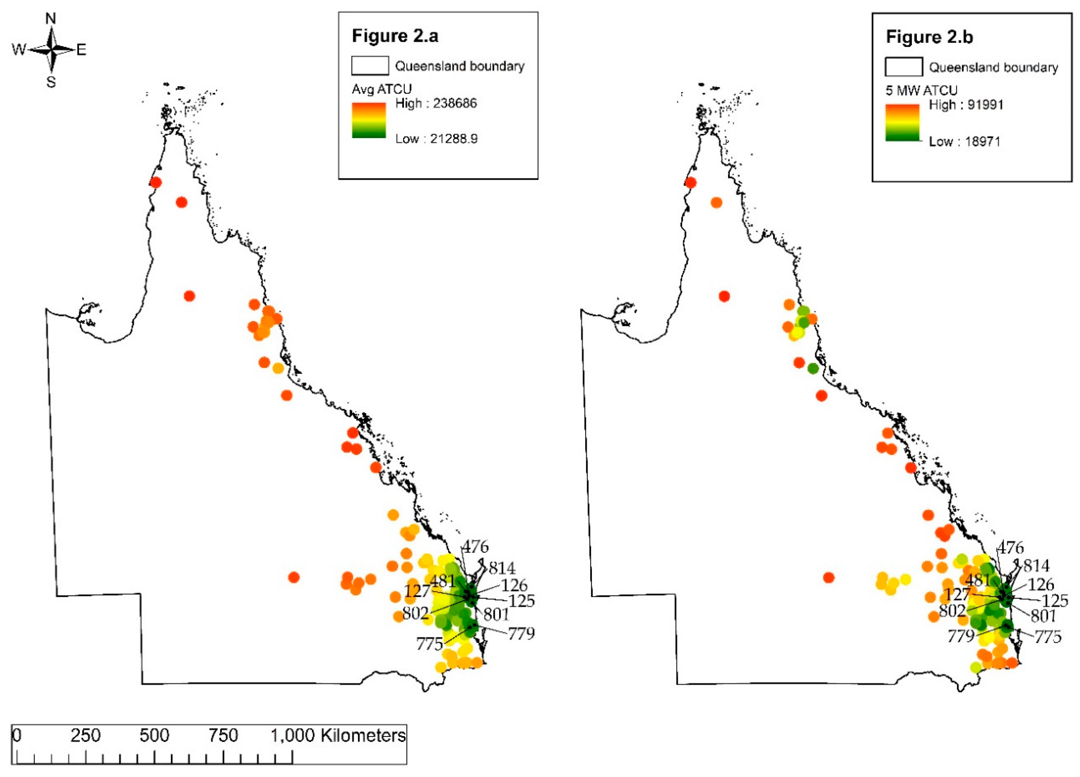
3.1. GIS Analysis: Strategic Facility Locations

The total harvestable area of forest in Queensland is estimated to be 13.6 M ha, including both plantations and native forests. The total amount of forest biomass energy is estimated to be 732 MW. The amount of energy is produced annually in plantations and native forests combined and includes the production of pulp logs, sawmill residues and field residues. The total harvestable forest footprint and total biomass energy are aggregated in an energy heatmap and used as inputs for LISA in the suitability analysis. This results in 844 administrative area polygons with significantly high biomass energy. The centroids of the 844 locations act as potential locations for bioenergy facilities. In testing the proximity to the road network (200 m), only 131 locations are eligible. Three out of the 131 locations are located on Bribie Island and were excluded in further analysis due to connectivity issues. There are 128 strategic facility locations for bioenergy purposes in the state of Queensland.

3.2. Model Analysis: Optimal Facility Location

Table 1 presents the mean and standard deviation (Std Dev) of TCj, ATCUj, TDj and ATDUj values from 128 strategic locations over the different capacities. Potential demand levels from small capacity (5 MW) to high capacity (100 MW) for each location are tested. At each capacity level, we can determine what the average, minimum and maximum cost or distance per MW would be for transport if we were to open a facility.
TCj and TDj values increase exponentially with increasing capacity. Normalizing the TCj and TDj values by the capacity creates a linear trend and smaller values for interpretation.
Because each strategic location is evaluated separately, locations for possible facilities can be ranked according to the ATCUj or ATDUj values. The location with the lowest ATDUj or ATCUj is considered the most optimal location. From the results shown in Figure 2, we can identify which of the 128 facility locations has the lowest ATCUj and ATDUj across all capacities (5–100 MW) based on hierarchy ranking. The labels of the 10 best facilities are shown. The dots represent 128 strategic locations, ranked by colour from lowest (green) to highest (red) ATCUj. In Figure 2a, the ATCUj value is averaged across all capacities for each facility. In Figure 2b, the ATCUj of a 5-MW facility is presented for each facility. Figure 2a indicates that the most optimal locations for energy conversion are located in the southeast (green) and other locations (red) are not feasible. However, looking at one particular small capacity (5 MW) in Figure 2b, it appears that some locations in the north can also be considered optimal in addition to the southeast. Location “476” is the best performing location with the lowest ATCUj and ATDUj across the range of capacities (Figure 3). The extent of the network to satisfy location “476” at a range of capacities is presented in Figure 3. As the most optimal location, the network connections are minimal but grow with increasing capacity.

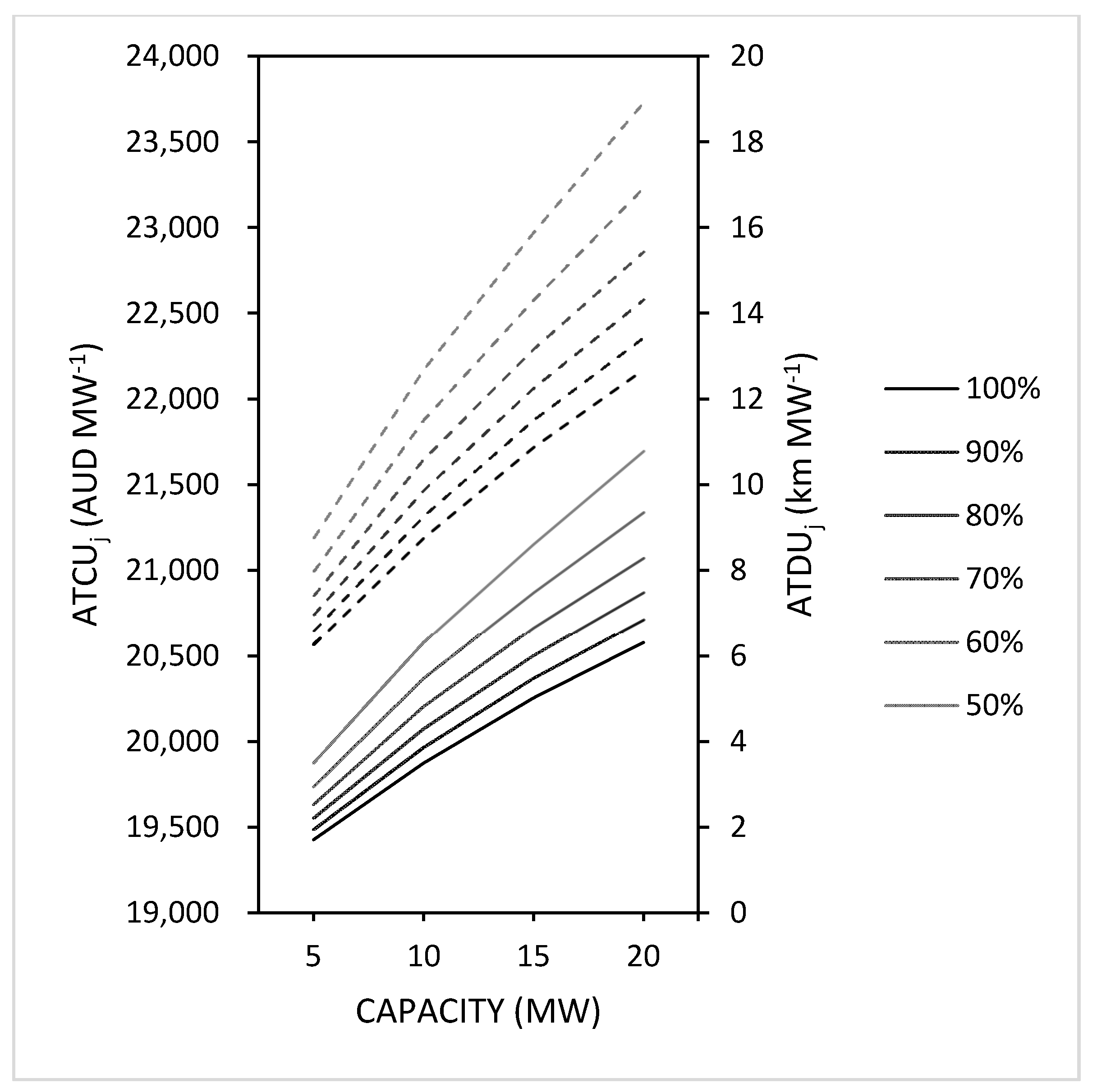
3.3. Sensitivity Analysis

3.3.1. Gate Price, Harvest and Stumpage Cost

The maximum transport cost is calculated for the base case (Scenario 1) as shown in Table 2. The base case scenario includes a stumpage cost of 0 AUD odt−1, a harvest cost of 48.25 AUD odt−1, and a gate price of 64.80 AUD odt−1. The maximum transport cost is 16.55 AUD odt−1 or converted to 25,200 AUD MW−1. The maximum transportation distance is 89 km and is the return distance from the facility to the forest.
Different combinations among gate price, harvest and stumpage cost are summarized in Table 2. Only the positive values of TCmax in Equation (7) are allowed to secure a profitable supply chain. Negative TCmax values are removed from Table 2. The remaining scenarios allow for the calculation of TDmax in Equation (8) and are presented in Table 2. We notice that only one scenario (10) with a stumpage cost of 28.27 AUD odt−1 remains. This means that combinations between this stumpage cost and other harvest costs and gate prices resulted in a negative value for TCmax. We also notice that none of the high harvest costs (77.16 AUD odt−1) are presented in the table, which means that these costs outweigh the price received for biomass and result in a loss in the supply chain.
In Figure 4, the maximum transport cost calculated in Table 2 for the base case scenario is compared to the mean of ATCUj values (J = 128) from the foregoing analysis (Table 1). For further comparison, the mean ATCUj of the ten (J = 10) best strategic locations (Figure 2) for each capacity is added to Figure 4. From the graph, it appears that, based on the calculated average, the 10 best locations remain under the maximum transport cost threshold (y = 25,200). Only at capacities above 90 MW does the curve exceed TCmax. On the other hand, the mean of all strategic locations exceeds TCmax at every capacity. This indicates that the average facility location in Queensland would not be profitable. However, in Table 3, the number of locations with ATCUj under TCmax are calculated and more detail indicates that, especially at lower capacities, a large set of locations can be feasible.
The maximum allowable capacity for a facility can be defined as the intersection between the average ATDUj of all strategic locations according to Equation (6) and TDmax calculated in the remaining scenarios (Table 2). In Figure 5, the mean ATDUj of all strategic locations is compared to the TDmax of the ten best scenarios. The dotted line y = 89 is the TDmax value of the base case scenario in Table 2. The point of intersection is at y = 89; x = 6, meaning that, based on the maximum return travel distance of 89 km MW−1, we could supply the average location in Queensland with up to 6 MW of forest biomass energy (CAPmax). With an increasing or decreasing gate price, stumpage or harvest cost, this maximum allowable capacity changes. Different values for TDmax in Table 2 are presented in Figure 5 (TDmax = y) and responding CAPmax values are indicated. Notice that at a maximum transport distance of 4 km (scenario 7), a negative capacity was retrieved and therefore this scenario cannot be sustained. For scenario 5, we find a maximum capacity of 0 MW, which also indicates that there is not enough supply within this distance cut-off to satisfy a facility. Table 4 presents the percentage of strategic locations (j) that fall under the maximum allowable transport distance (TDmax) for each scenario and the range of capacities. From the table, we can see that 99% of locations can be supplied with 5 MW if we were able to transport biomass over a total distance of 302 km in scenario 3. This percentage drops with increasing capacity and decreasing distance and becomes 0% when the maximum transport distance is reduced to 4 km and capacities are over 5 MW. Despite this, 1% of the locations are able to produce 5 MW of energy under a maximum transport distance of 4 km.

3.3.2. Biomass Availability

The effect of reduced availabilities from 100% to 50% is tested on the mean ATCUj and ATDUj of the 10 best strategic locations with a decrement of 10%. For the sake of simplicity, the mean ATCUj and ATDUj are only calculated for capacities of 5, 10, 15 and 20 MW and are presented in Figure 6. For example, the ATCUj of location “476” at 20 MW and 100% availability is 20,300 AUD MW−1 and increases to 21,200 AUD MW−1 at the same capacity with only 50% of the biomass available. For location “801” the ATDUj is 3.73 km MW−1 at 100% biomass availability and 5 MW capacity and increases to 5.99 km MW−1 at the same capacity with only 50% of the biomass available.
From the foregoing analysis and according to Figure 2, location “476” is the overall best performing location on different capacities (5–100 MW). However, according to Table 5, location “801” is the most optimal at 100% biomass availability and low capacities (5–20 MW). With decreasing biomass availability, however, longer distances will need to be covered to satisfy the potential demand of the facility. At reduced biomass availability and increasing capacity, locations “125” and “476” become more favourable (Table 5).

3.3.3. Fuel Price

The ATCUj of the ten best facilities is calculated accordingly for the low and high fuel scenario (Equations (9) and (10)) and compared with the average fuel price in Figure 7. For example, the ATCUj of location “476” at 20 MW and average fuel price is 20,300 AUD MW−1 and increases to 20,700 AUD MW−1 with a high fuel price and drops to 19,800 AUD MW−1 with a low fuel price. At a low capacity (5 MW), both the high and low fuel prices result in a 1% change in the ATCUj value. At a high capacity (100 MW) this results in a 7% decrement of ATCUj for low fuel price and a 6% increment of ATCUj for the high fuel price.

4. Discussion

This research combines GIS methods with a transportation cost model to find the optimal location of forest biomass-to-bioenergy facilities. In considering the development of a profitable bioenergy facility that can sustainably produce bioenergy from forest biomass: (i) there has to be enough biomass to supply the bioenergy facility, and (ii) the biomass has to be sourced within a sensible distance at the lowest possible cost. The two-stage DSS helps to address this biomass logistics problem and this research demonstrates the method in the large study region of Queensland, Australia. The spatial component preceding the transportation cost model indicated that 732 MW of forest biomass is available per year and identified 128 strategic locations to covert this biomass into energy products. Similar quantities for biomass availability can be found in the Australian literature for the state of Queensland [65,66,67] and are roughly converted to one million dry tonnes of forest biomass. Each of the strategic locations served as inputs for the transportation cost model and further location optimization. In the literature [19,20,27], GIS-based methods have been used numerous times to assess biomass and to identify locations for biomass conversion, but seldom have they been applied to such a large-scale extent. Since the transportation of biomass is an overwhelming contributor to biomass supply chain costs [25], further refinement of strategic locations based on transport cost and distance provides a more optimal solution to the facility location problem.
By calculating the average transportation cost and distance of the strategic locations retrieved from the GIS analysis, this research can identify the most optimal location for a forest biomass-to-bioenergy facility if we were to establish one. A similar approach was applied to finding the optimal location to convert forest biomass to biofuel by Zhang et al. [27]. The most optimal location for a facility would be the facility with the lowest transport cost and distance at the required capacity. However, understanding that one facility is necessary to capture the entire supply over large areas such as Queensland is complex and a challenging task. Even though the rationale of the transportation cost model is to minimize the cost of transport, our additional motivation is to maximize the capacity within the study area. In the ideal scenario, the cost of supply is kept minimal and the biomass that is produced within the forest is utilized to the greatest possible extent by the bioenergy facility. The combination of GIS and a transportation cost model allows us to tackle this problem. The ATCUj that is calculated for each facility at a range of capacities is low when either the cost of transport is minimal, or the supplied capacity is great (AUD MW−1). Thus, the ATCUj value is an indicator of the optimal facility location problem. For comparison, the study by Zhang et al. [27] found a total cost value of USD 4.32 M for a facility using 635,000 tonnes (50% moisture) of forest biomass. The ATCUj value from their result converts to 31,100 AUD MW−1 for the best facility. In our research, location “476” was found to be the best performing across a range of capacities and has an ATCUj value of 22,300 AUD MW−1, which is located in the most biomass-dense area of the study region.
To understand the effect of price and cost changes in the biomass supply, the results of the transportation cost model were compared to the maximum cost and distance of the biomass supply chain. Values for gate price, harvest cost, and stumpage cost can vary significantly based on the type of harvest system, forest type, type of forest biomass or tree species, amount of biomass, equipment or even the deployment of biomass used in the area. The cost of harvest, stumpage and the gate price of forest biomass are not included as integral parts of the transportation model; however, they are incorporated as constraining elements to secure the profit of the forest biomass market. According to different cost price scenarios in relation to sensitivity, the maximum allowable transport cost and distance will vary and are independent of the capacity. This research estimated that the maximum allowable transport cost is 25,200 AUD MW−1 and the maximum allowable transport distance is an 89 km MW return journey. We found one other research example in Australia that indicated a range of costs between 48.32 AUD odt−1 and 63.25 AUD odt−1 for hardwood chips for delivering biomass residues over a transport distance of 90 km [68]. When converted, the 89-km maximum allowable transport distance in this research corresponds to a maximum transport cost of 16.55 AUD odt−1. When we convert and add the cost of harvest (48.35 AUD odt−1) to the transport cost we receive a comparable value of 64.80 AUD odt−1. The point of intersection between the 89-km maximum allowable transport distance and the average transportation distance per megawatt according to the transportation analysis is at a capacity of 6 MW. Thus, under the circumstance of the base case scenario, the average facility in Queensland becomes less profitable beyond this capacity when keeping in mind that this is based on the average of the best and worst performing locations. The introduction of a maximum allowable transport costs creates a benchmark for the strategic facility locations from the transportation cost model. When the benchmark cost or distance is exceeded, the strategic location can be rejected as an optimal solution.
To examine the sensitivity of decisions to changes in biomass availability and the cost of fuel, the transportation cost model was also executed by changing these parameters. The biomass availability can suffer considerable losses due to alternative uses; hence, this research investigated 10% decrements of biomass availability. By reducing the availability of biomass supply, the preference of location shifts. With less biomass available, more biomass needs to be collected from additional forest locations. This affects the result of the transportation cost model by increasing the cost due to increased transport distances or reducing the supplied capacity. The optimal facility location is therefore characterized by an increasing ATCUj value. On average, for a 5-MW facility, a reduction of 10% in the biomass availability resulted in an ATCUj increase of 90 AUD MW−1. The cost of fuel can change significantly throughout the year. Cyclical changes in fuel price, sometimes up to 20%, are not uncommon and have a significant impact on the cost of transport and the fleet. Changes in fuel prices do not interfere at a capacity level of a facility or the supply of biomass to a facility. However, changes in fuel price will affect the ATCUj value from the transportation cost model and simultaneously impact the maximum allowable transportation distance. Changes in the ATCUj value up to 7% were recorded in this study based on changes in fuel price. Similar to the results found in Zhang et al. [27], a change in fuel price did not affect the optimal location, as opposed to changes in biomass availability.
There are several possible opportunities for future research to extend and enhance the developed DSS. One of the key opportunities is to take the single-facility transportation problem to a multi-facility optimization scenario, thereby focusing on utilizing as much of the forest biomass as possible throughout the study area by selecting multiple optimal locations for the conversion of biomass. It is important to consider that each potential facility can be supplied with biomass from within its service area at the lowest possible cost without competition between these facilities. Such models can reinforce the decision on the number of facilities and required capacity needed in the study area to maximize the demand, while minimizing the cost. Often, there will be limits to a capacity of a facility, so it is worth considering a minimum and maximum capacity level based on the technology and biomass resource. When optimizing the supply chain, research should consider economic, environmental and social aspects to come up with the best possible scenario. Depending on the geographical location, interruptions of the forest biomass supply occur annually due to spring/breeding season, snow or fire seasons. It is therefore recommended to improve the knowledge of biomass availability by simulating the annual harvesting cycles and biomass storage solutions.

5. Conclusions

This paper demonstrated the use of a two-stage decision support system that finds the optimal location of forest biomass-to-bioenergy facilities based on available biomass, transport distance, and transport cost in the study area of Queensland. In stage 1, the method identified 128 strategic locations using a GIS approach. In stage 2, the optimal location for forest biomass-to-bioenergy conversion was based upon reduced transport costs. The influence of fuel price, biomass availability, and cost and pricing of the biomass supply chain was evaluated through a series of sensitivity analyses.
From the case study, we can conclude that:
  • Location “476” was identified to be the optimal location for bioenergy production from forest biomass across a range of facility capacities.
  • The ATCUj of the average facility in Queensland ranges from 33,700 AUD MW−1 at 5 MW capacity to 79,400 AUD MW−1 at 100 MW with an ATDUj of 86 km MW−1 at 5 MW and 341 km MW−1 at 100 MW.
  • The sensitivity analysis showed that fuel prices and biomass availability have an influence on the transport cost. Biomass availability also influences the selection of the optimal facility location. At the lowest capacity level and 100% biomass availability, location “801” was the optimal location; with increasing capacity or reduced availability, location “476” was the optimal site.
  • The sensitivity analysis also showed that changes in the biomass price and the costs of the supply chain have an impact on the maximum allowable transport distance and cost. In the base case, the maximum allowable transport distance for a facility in Queensland is 89 km MW−1 and the maximum allowable transport cost is 25,200 AUD MW−1.
The use of a two-stage DSS for the selection of an optimal facility location has been demonstrated. Additionally, the method evaluated every other possible location and created an average performance scenario for the case area, which enables future planning, investigation and investment from a strategic perspective. The single-facility transportation cost model can be extended to optimization methods that allow for multiple facilities to coexist. The method can potentially be extended to other regions and biomass scenarios.

Author Contributions

Conceptualization, S.V.H. and D.R.; methodology, S.V.H., S.E., D.R. and M.B.; software, S.V.H.; formal analysis, S.V.H.; investigation, S.V.H. and S.E.; resources, S.V.H. and M.B.; data curation, S.V.H.; writing—original draft preparation, S.V.H.; writing—review and editing, S.E., D.R. and M.B.; visualization, S.V.H.; supervision, S.E., D.R. and M.B.; funding acquisition, M.B. All authors have read and agreed to the published version of the manuscript.

Funding

This research was funded by the Australian Biomass for Bioenergy Assessment (ABBA) as part of the Australian Renewable Energy Agency (ARENA) through a University of the Sunshine Coast Research Scholarship (USCRS-ABBA), grant number (PRJ-010376).

Acknowledgments

We want to thank the anonymous reviewers and the journal editor for taking their time to review and provide valuable input and comments. The Gottstein Trust provided additional funding through a forest industry top-up scholarship.

Conflicts of Interest

The authors declare no conflict of interest. The funders had no role in the design of the study; in the collection, analyses, or interpretation of data; in the writing of the manuscript, or in the decision to publish the results.

Appendix A

Due to the lack of case study examples in Australia, values for gate price, harvest, and stumpage cost were collected from the literature and personal communications. All the values have been converted to AUD odt−1 as this is the most used unit for biomass delivery costs. For the developed DSS method, these unit costs are converted to AUD MW−1 to be comparable at a facility capacity (MW) level, by using a conversion factor of 1520 odt MW−1.
  • Harvest cost:
    48.25 AUD odt−1: Base case or reference cost value. Calculated according to the weighted average of total native forest biomass (356,376 odt) and plantation forest biomass (756,468 odt) in the case study area of Queensland. The average harvest cost for plantation biomass is estimated to be 38.37 AUD odt−1 according to the average of two case studies in Australia. Case study one is a softwood plantation cut-to-length harvesting system in the Green Triangle, Australia [69] with harvest, extraction and onsite chipping. Case study two is an integrated harvest operation with harvest, extraction and onsite chipping in pine plantations in Western Australia using the Fibreplus method [70]. The harvesting cost of native forest biomass is estimated to be 69.23 AUD odt−1 for Queensland specifically, according to a personal communication [71].
    37.29 AUD odt−1: Low-cost case. Calculated according to the weighted average of total native forest and plantation forest biomass in Queensland. The average harvest cost for plantation biomass is estimated to be 22.25 AUD odt−1 according to the average of three case studies in Australia. Case study one is a hardwood plantation cut-to-length harvesting system in the Green Triangle, Australia [69] with harvest, extraction and chipping at the mill. Case study two is a hardwood plantation whole-tree harvesting system in the Green Triangle, Australia [69] with harvest, extraction and chipping at the mill. Case study three is an integrated harvest operation with harvest, extraction and chipping at the mill in pine plantations in Western Australia using the Fibreplus method [70]. The harvesting cost of native forest biomass is estimated to be 69.23 AUD odt−1 for Queensland specifically, according to a personal communication [71].
    77.16 AUD odt−1: High-cost case. Calculated according to the weighted average of total native forest and plantation forest biomass in Queensland. The average harvest cost for plantation biomass is estimated to be 80.90 AUD odt−1 according to the average of two case studies in Australia. Case study one is a softwood plantation cut-to-length harvesting system in Victoria with harvest, extraction and roadside chipping (Bruks Chipper) [72]. Case study two is a softwood plantation cut-to-length harvesting system in Victoria with harvest and in-field chipping (Bruks Chipper) [73]. The harvesting cost of native forest biomass is estimated to be 69.23 AUD odt−1 for Queensland specifically, according to a personal communication [71].
  • Stumpage cost:
    0.00 AUD odt−1: Base case or reference cost value. There is currently no stumpage cost paid to the landowner for forest biomass.
    10.00 AUD odt−1: Moderate-cost case based on a trial in Western Australia where the industry was asked what they would pay for biomass from the roadside [74].
    28.27 AUD odt−1: High-cost case based on the average between the stumpage price for pulp logs in Queensland for pulp and paper industry [75] and the stumpage price for hardwood forest residues in Tasmania [76].
  • Gate price:
    64.80 AUD odt−1: Base case or reference price value. This value is based on international references and personal communication [74,77]
    50.40 AUD odt−1: Low-price case according to a review case in Australia [12]
    79.00 AUD odt−1: High-price case according to a case example in the Green Triangle, Australia [69].

References

  1. Australian Government Forests. Wood and Australia’s Carbon Balance. In CRC Greenhouse Accounting; Australian Government Forest and Wood Products Research and Development Corporation: Canberra, Australia, 2006. [Google Scholar]
  2. ABARES. Australia’s State of the Forests Report 2018; Australian Government Department of Agriculture and Water Resources: Canberra, Australia, 2018.
  3. Berndes, G.; Abts, B.; Asikainen, A.; Cowie, A.; Dale, V.; Egnell, G.; Lindner, M.; Marelli, L.; Paré, D.; Pingoud, K.; et al. Forest Biomass, Carbon Neutrality and Climate Change Mitigation; European Forest Institute: Joensuu, Finland, 2016. [Google Scholar]
  4. IEA Bioenergy. Sustainable Production of Woody Biomass for Energy; A Position Paper Prepared by IEA Bioenergy; IEA Bioenergy: Rotorua, New Zealand, 2002; Volume 3. [Google Scholar]
  5. Sharma, B.; Ingalls, R.G.; Jones, C.L.; Khanchi, A. Biomass supply chain design and analysis: Basis, overview, modeling, challenges, and future. Renew. Sustain. Energy Rev. 2013, 24, 608–627. [Google Scholar] [CrossRef]
  6. Bridgwater, A.V.; Toft, A.J.; Brammer, J.G. A techno-economic comparison of power production by biomass fast pyrolysis with gasification and combustion. Renew. Sustain. Energy Rev. 2002, 6, 181–246. [Google Scholar] [CrossRef]
  7. Raison, R.J. Opportunities and impediments to the expansion of forest bioenergy in Australia. Biomass Bioenergy 2006, 30, 1021–1024. [Google Scholar] [CrossRef]
  8. KPMG. Bioenergy State of the Nation Report; Bioenergy Australia: Canberra, Australia, 2018. [Google Scholar]
  9. Department of the Environment and Energy. Australian Energy Update 2018; Australian Government: Canberra, Australia, 2018.
  10. Zhang, F.; Wang, J.; Liu, S.; Zhang, S.; Sutherland, J.W. Integrating GIS with optimization method for a biofuel feedstock supply chain. Biomass Bioenergy 2017, 98, 194–205. [Google Scholar] [CrossRef]
  11. De Meyer, A.; Cattrysse, D.; Rasinmäki, J.; Van Orshoven, J. Methods to optimise the design and management of biomass-for-bioenergy supply chains: A review. Renew. Sustain. Energy Rev. 2014, 31, 657–670. [Google Scholar] [CrossRef] [Green Version]
  12. Ghaffariyan, M.R.; Brown, M.; Acuna, M.; Sessions, J.; Gallagher, T.; Kühmaier, M.; Spinelli, R.; Visser, R.; Devlin, G.; Eliasson, L.; et al. An international review of the most productive and cost effective forest biomass recovery technologies and supply chains. Renew. Sustain. Energy Rev. 2017, 74, 145–158. [Google Scholar] [CrossRef]
  13. Shabani, N.; Akhtari, S.; Sowlati, T. Value chain optimization of forest biomass for bioenergy production: A review. Renew. Sustain. Energy Rev. 2013, 23, 299–311. [Google Scholar] [CrossRef]
  14. Iakovou, E.; Karagiannidis, A.; Vlachos, D.; Toka, A.; Malamakis, A. Waste biomass-to-energy supply chain management: A critical synthesis. Waste Manag. 2010, 30, 1860–1870. [Google Scholar] [CrossRef]
  15. Mafakheri, F.; Nasiri, F. Modeling of biomass-to-energy supply chain operations: Applications, challenges and research directions. Energy Policy 2014, 67, 116–126. [Google Scholar] [CrossRef]
  16. Shi, X.; Elmore, A.; Li, X.; Gorence, N.J.; Jin, H.; Zhang, X.; Wang, F. Using spatial information technologies to select sites for biomass power plants: A case study in Guangdong Province, China. Biomass Bioenergy 2008, 32, 35–43. [Google Scholar] [CrossRef]
  17. Hock, B.K.; Blomqvist, L.; Hall, P.; Jack, M.; Möller, B.; Wakelin, S.J. Understanding forest-derived biomass supply with GIS modelling. J. Spat. Sci. 2012, 57, 213–232. [Google Scholar] [CrossRef]
  18. Acuna, M. Timber and biomass transport optimization: A review of planning issues, solution techniques and decision support tools. Croat. J. For. Eng. 2017, 38, 279–290. [Google Scholar]
  19. Ranta, T. Logging residues from regeneration fellings for biofuel production-a GIS-based availability analysis in Finland. Biomass Bioenergy 2005, 28, 171–182. [Google Scholar] [CrossRef]
  20. Voivontas, D.; Assimacopoulos, D.; Koukios, E.G. Assessment of biomass potential for power production: A GIS based method. Biomass Bioenergy 2001, 20, 101–112. [Google Scholar] [CrossRef]
  21. Han, H.; Chung, W.; Wells, L.; Anderson, N. Optimizing biomass feedstock logistics for forest residue processing and transportation on a tree-shaped road network. Forests 2018, 9, 121. [Google Scholar] [CrossRef] [Green Version]
  22. Anderson, N.; Chung, W.; Loeffler, D.; Jones, J.G. A productivity and cost comparison of two systems for producing biomass fuel from roadside forest treatment residues. For. Prod. J. 2012, 62, 222–233. [Google Scholar] [CrossRef] [Green Version]
  23. Visser, R.; Berkett, H.; Spinelli, R. Determining the effect of storage conditions on the natural drying of radiata pine logs for energy use. N. Z. J. For. Sci. 2014, 44, 1–8. [Google Scholar] [CrossRef] [Green Version]
  24. Acuna, M.; Anttila, P.; Sikanen, L.; Prinz, R.; Asikainen, A. Predicting and controlling moisture content to optimise forest biomass logistics. Croat. J. For. Eng. 2012, 33, 225–238. [Google Scholar]
  25. Noon, C.E.; Daly, M.J. GIS-based biomass resource assessment with BRAVO. Biomass Bioenergy 1996, 10, 101–109. [Google Scholar] [CrossRef]
  26. Awudu, I.; Zhang, J. Uncertainties and sustainability concepts in biofuel supply chain management: A review. Renew. Sustain. Energy Rev. 2012, 16, 1359–1368. [Google Scholar] [CrossRef]
  27. Zhang, F.; Johnson, D.M.; Sutherland, J.W. A GIS-based method for identifying the optimal location for a facility to convert forest biomass to biofuel. Biomass Bioenergy 2011, 35, 3951–3961. [Google Scholar] [CrossRef]
  28. Akhtari, S.; Sowlati, T.; Griess, V.C. Integrated strategic and tactical optimization of forest-based biomass supply chains to consider medium-term supply and demand variations. Appl. Energy 2018, 213, 626–638. [Google Scholar] [CrossRef]
  29. Perpiña, C.; Martínez-Llario, J.C.; Pérez-Navarro, Á. Multicriteria assessment in GIS environments for siting biomass plants. Land Use Policy 2013, 31, 326–335. [Google Scholar] [CrossRef]
  30. Comber, A.; Dickie, J.; Jarvis, C.; Phillips, M.; Tansey, K. Locating bioenergy facilities using a modified GIS-based location-allocation-algorithm: Considering the spatial distribution of resource supply. Appl. Energy 2015, 154, 309–316. [Google Scholar] [CrossRef] [Green Version]
  31. Buchholz, T.; Rametsteiner, E.; Volk, T.A.; Luzadis, V.A. Multi Criteria Analysis for bioenergy systems assessments. Energy Policy 2009, 37, 484–495. [Google Scholar] [CrossRef]
  32. Jiang, H.; Eastman, J.R. Application of fuzzy measures in multi-criteria evaluation in GIS. Int. J. Geogr. Inf. Sci. 2000, 14, 173–184. [Google Scholar] [CrossRef]
  33. Woo, H.; Acuna, M.; Moroni, M.; Taskhiri, M.S.; Turner, P. Optimizing the location of biomass energy facilities by integrating Multi-Criteria Analysis (MCA) and Geographical Information Systems (GIS). Forests 2018, 9, 585. [Google Scholar] [CrossRef] [Green Version]
  34. Delivand, M.K.; Cammerino, A.R.B.; Garofalo, P.; Monteleone, M. Optimal locations of bioenergy facilities, biomass spatial availability, logistics costs and GHG (greenhouse gas) emissions: A case study on electricity productions in South Italy. J. Clean. Prod. 2015, 99, 129–139. [Google Scholar] [CrossRef]
  35. Mladenović, N.; Brimberg, J.; Hansen, P.; Moreno-Pérez, J.A. The p-median problem: A survey of metaheuristic approaches. Eur. J. Oper. Res. 2007, 179, 927–939. [Google Scholar] [CrossRef] [Green Version]
  36. Current, J.R.; Re Velle, C.S.; Cohon, J.L. The maximum covering/shortest path problem: A multiobjective network design and routing formulation. Eur. J. Oper. Res. 1985, 21, 189–199. [Google Scholar] [CrossRef]
  37. Brimberg, J.; Hansen, P.; Mladenović, N.; Taillard, E.D. Improvements and Comparison of Heuristics for Solving the Uncapacitated Multisource Weber Problem. Oper. Res. 2000, 48, 444–460. [Google Scholar] [CrossRef]
  38. Zhan, F.B.; Chen, X.; Noon, C.E.; Wu, G. A GIS-enabled comparison of fixed and discriminatory pricing strategies for potential switchgrass-to-ethanol conversion facilities in Alabama. Biomass Bioenergy 2005, 28, 295–306. [Google Scholar] [CrossRef]
  39. Guilhermino, A.; Lourinho, G.; Brito, P.; Almeida, N. Assessment of the Use of Forest Biomass Residues for Bioenergy in Alto Alentejo, Portugal: Logistics, Economic and Financial Perspectives. Waste Biomass Valorization 2018, 9, 739–753. [Google Scholar] [CrossRef]
  40. Frombo, F.; Minciardi, R.; Robba, M.; Rosso, F.; Sacile, R. Planning woody biomass logistics for energy production: A strategic decision model. Biomass Bioenergy 2009, 33, 372–383. [Google Scholar] [CrossRef]
  41. Nord-Larsen, T.; Talbot, B. Assessment of forest-fuel resources in Denmark: Technical and economic availability. Biomass Bioenergy 2004, 27, 97–109. [Google Scholar] [CrossRef]
  42. Freppaz, D.; Minciardi, R.; Robba, M.; Rovatti, M.; Sacile, R.; Taramasso, A. Optimizing forest biomass exploitation for energy supply at a regional level. Biomass Bioenergy 2004, 26, 15–25. [Google Scholar] [CrossRef]
  43. Van Holsbeeck, S.; Srivastava, S.K. Feasibility of locating biomass-to-bioenergy conversion facilities using spatial information technologies: A case study on forest biomass in Queensland, Australia. Biomass Bioenergy 2020, 139, 105620. [Google Scholar] [CrossRef]
  44. Anselin, L. Local Indicators of Spatial Association—LISA. Geogr. Anal. 1995, 27, 93–115. [Google Scholar] [CrossRef]
  45. Dijkstra, E.W. A Note on Two Problems in Connexion with Graphs. Numer. Math. 1959, 1, 269–271. [Google Scholar] [CrossRef] [Green Version]
  46. [Dataset] Mark Brown; University of the Sunshine Coast, Sippy Downs, QLD, Australia. Personal communication, 22 August 2019.
  47. NHVR. Common Heavy Freight Vehicle Configurations; National Heavy Vehicle Regulator: Brisbane, Australia, 2019. [Google Scholar]
  48. RACQ. Annual Fuel Price Report 2019; Royal Automobile Club of Queensland: Eight Mile Plains, Australia, 2020. [Google Scholar]
  49. Department of Agriculture and Fisheries. Forest Products Pocket Facts—2017; Queensland Government: Brisbane, Australia, 2017.
  50. Department of Agriculture and Fisheries. Queensland Forest & Timber Industry; Queensland Government: Brisbane, Australia, 2016.
  51. [Dataset] ABARES Australian Forest and Wood Products Statistics—March and June Quarters 2019. Available online: https://www.agriculture.gov.au/abares/research-topics/forests/forest-economics/forest-wood-products-statistics (accessed on 30 April 2020).
  52. Lock, P.; Whittle, L. Future Opportunities for Using Forest and Sawmill Residues in Australia; Australian Government Department of Agriculture and Water Resources: Canberra, Australia, 2018.
  53. Altus Renewables. Available online: https://www.altusrenewables.com (accessed on 5 May 2020).
  54. Department of the Environment and Energy. Australian Energy Statistics, Table O; Australian Government: Canberra, Australia, 2019.
  55. [Dataset] ABARES Australian Forest and Wood Products Statistics: March and June Quarters 2018. Available online: https://www.agriculture.gov.au/abares/research-topics/forests/forest-economics/forest-wood-products-statistics (accessed on 5 April 2019).
  56. [Dataset] Queensland Government Queensland Spatial Catalogue-QSpatial: Agricultural Land Audit-Potential Softwood Plantation Forestry-Queensland. Available online: https://www.daf.qld.gov.au/archive/business-priorities/environment/ag-land-audit (accessed on 9 September 2019).
  57. [Dataset] Queensland Government Open Data Portal: Agricultural Land Audit-Potential Native Forestry-Queensland 2019. Available online: https://www.data.qld.gov.au/dataset/agricultural-land-audit-queensland-series/resource/7ea4aeec-54bf-4fcc-9cd2-827d984163d (accessed on 9 September 2019).
  58. [Dataset] ABARES Forests of Australia. Available online: http://www.agriculture.gov.au/abares/forestsaustralia/forest-data-maps-and-tools/spatial-data/forest-cover (accessed on 9 September 2019).
  59. [Dataset] Queensland Government Queensland Spatial Catalogue-QSpatial: Agricultural Land Audit-Potential Hardwood Plantation Forestry-Queensland. Available online: http://qldspatial.information.qld.gov.au/catalogue/custom/index.page (accessed on 9 September 2019).
  60. Neldner, V.J.; Niehus, R.E.; Wilson, B.A.; McDonald, W.J.F.; Ford, A.J.; Accad, A. The Vegetation of Queensland. Descriptions of Broad Vegetation Groups, Version 3; Queensland Government: Brisbane, Australia, 2017.
  61. [Dataset] Geoscience Australia GEODATA TOPO 20K Series 3. Bioregional Assessment Source Dataset 2006. Available online: https://data.gov.au/data/dataset/a0650f18-518a-4b99-a553-44f82f28bb5f (accessed on 9 September 2019).
  62. Australian Bureau of Statistics Australian Statistical Geography Standard (ASGS): Volume 1. Available online: https://www.abs.gov.au/ausstats/abs@.nsf/mf/1270.0.55.001 (accessed on 9 September 2019).
  63. ESRI. ArcGIS Desktop 10.7; Esri Australia Pty. Ltd.: Brisbane, QLD, Australia, 2020. [Google Scholar]
  64. LINDO. What’sBest! 16.0; LINDO Systems, Inc.: Chicago, IL, USA, 2020. [Google Scholar]
  65. Farine, D.R.; O’Connell, D.A.; Raison, R.J.; May, B.M.; O’Connor, M.H.; Crawford, D.F.; Herr, A.; Taylor, J.A.; Jovanovic, T.; Campbell, P.K.; et al. An assessment of biomass for bioelectricity and biofuel, and for greenhouse gas emission reduction in Australia. GCB Bioenergy 2012, 4, 148–175. [Google Scholar] [CrossRef]
  66. Crawford, D.F.; O’Connor, M.H.; Jovanovic, T.; Herr, A.; Raison, R.J.; O’Connell, D.A.; Baynes, T. A spatial assessment of potential biomass for bioenergy in Australia in 2010, and possible expansion by 2030 and 2050. GCB Bioenergy 2016, 8, 707–722. [Google Scholar] [CrossRef]
  67. Department of Science Information Technology and Innovation. Australian Biomass for Bioenergy Assessment Queensland Technical Methods—Forestry; Queensland Government: Brisbane, Australia, 2017.
  68. IndustryEdge. Australian Hardwood Chip Export Volume & Price Forecasts and Stumpage and Harvest Cost Review; IndustryEdge Pty Ltd.: Geelong West, Australia, 2013. [Google Scholar]
  69. Rodriguez, L.C.; May, B.; Herr, A.; O’Connell, D. Biomass assessment and small scale biomass fired electricity generation in the Green Triangle, Australia. Biomass Bioenergy 2011, 35, 2589–2599. [Google Scholar] [CrossRef]
  70. Ghaffariyan, M.R.; Spinelli, R.; Magagnotti, N.; Brown, M. Integrated harvesting for conventional log and energy wood assortments: A case study in a pine plantation in Western Australia. South. For. J. For. Sci. 2015, 77, 249–254. [Google Scholar] [CrossRef]
  71. Ryan, S.; Private Forestry Service Queensland, Gympie, QLD, Australia. Personal communication, 2020.
  72. Ghaffariyan, M.R.; Sessions, J.; Brown, M. Evaluating productivity, cost, chip quality and biomass recovery for a mobile chipper in Australian roadside chipping operations. J. For. Sci. 2012, 58, 530–535. [Google Scholar] [CrossRef] [Green Version]
  73. Ghaffariyan, M.R.; Sessions, J.; Brown, M. Collecting harvesting residues in pine plantations using a mobile chipper in Victoria (Australia). Silva Balc. 2014, 15, 81–95. [Google Scholar]
  74. Brown, M.; University of the Sunshine Coast, Sippy Downs, QLD, Australia. Personal communication, 2020.
  75. KPMG. Australian Pine Log Price Index (Stumpage) Updated to June 2017; HVP Plantations: Myrtleford, Australia, 2017. [Google Scholar]
  76. Rothe, A.; Moroni, M.; Neyland, M.; Wilnhammer, M. Current and potential use of forest biomass for energy in Tasmania. Biomass Bioenergy 2015, 80, 162–172. [Google Scholar] [CrossRef]
  77. Yoshioka, T.; Sakurai, R.; Kameyama, S.; Inoue, K.; Hartsough, B. The optimum slash pile size for grinding operations: Grapple excavator and horizontal grinder operations model based on a Sierra Nevada, California Survey. Forests 2017, 8, 442. [Google Scholar] [CrossRef] [Green Version]
Figure 1. An overview of the developed methodology.
Forests 11 00968 g001
Figure 2. (a) Strategic facility locations indexed by the average ATCUj calculated over a 5–100 MW capacity range. (b) Strategic facility locations indexed by the ATCUj at 5 MW. The 10 best locations with the lowest ATCUj across all capacities are labelled.
Forests 11 00968 g002
Figure 3. Location “476” and its respective connection with the forest to satisfy respective capacities of 5, 10, 20, 50 and 100 MW.
Forests 11 00968 g003
Figure 4. Comparison between mean ATCUj, mean ATCUj of the ten best strategic locations and TCmax of the base case scenario.
Forests 11 00968 g004
Figure 5. Comparison between mean ATDUj and TDmax of different price-cost scenarios.
Forests 11 00968 g005
Figure 6. Sensitivity of mean ATCUj (solid line) and mean ATDUj (dotted line) of the ten best facilities to reduced biomass availability.
Forests 11 00968 g006
Figure 7. Sensitivity of mean ATCUj of ten best strategic locations to changes in fuel price.
Forests 11 00968 g007
Table 1. Mean jth demand point (TCj), average transportation cost per unit of biomass (AUD MW−1) for the jth demand point, (ATCUj), total transportation distance for the jth demand point (TDj), average transportation distance per unit of biomass (km MW−1) for a given facility site (ATDUj) and SD values of 128 strategic locations for different capacities in Queensland.
Capacity LevelTCj (AUD)ATCUj (AUD MW−1)TDj (km)ATDUj (km MW−1)
(MW)MeanStd DevMeanStd DevMeanStd DevMeanStd Dev
5169,00067,20033,70013,4004303758675
10387,000182,00038,70018,20011401010114101
15634,000334,00042,30022,30020001860134124
20907,000513,00045,40025,70030202860151143
301,510,000917,00050,50030,60053805110179170
402,170,0001,370,00054,20034,10080007610200190
502,880,0001,850,00057,60037,10010,90010,300219207
603,650,0002,380,00060,90039,60014,20013,200237221
704,540,0002,980,00064,90042,60018,20016,600260237
805,560,0003,760,00069,50047,00022,80020,900285262
906,710,0004,820,00074,60053,50028,20026,900314298
1007,940,0006,030,00079,40060,30034,10033,600341336
Table 2. Estimated maximum transport cost (TCmax) and maximum allowable transport distance (TDmax) values for a range of scenarios based on changes in gate price, stumpage and harvest costs.
ScenarioStumpage Cost
(AUD odt−1)
Harvest Cost
(AUD odt−1)
Gate Price
(AUD odt−1)
TCmax
(AUD odt−1)
TCmax
(AUD MW−1)
TDmax
(km MW−1)
1 (base)0.0048.2564.8016.5525,20089
20.0048.2579.0030.7546,700210
30.0037.2979.0041.7163,400302
40.0037.2964.8027.5141,800182
50.0037.2950.4013.1119,90060
610.0048.2579.0020.7531,500125
710.0048.2564.806.5599604
810.0037.2979.0031.7148,200218
910.0037.2964.8017.5126,60097
1028.2737.2979.0013.4420,40063
Table 3. Number of strategic locations (J) performing under TCmax of the base case scenario.
Capacity (MW)510152030405060708090100
J under TCmax4133282417161616101077
J = 12832%26%22%19%13%13%13%13%8%8%5%5%
Table 4. Percentage of strategic locations performing under the respective TDmax scenarios over a range of different capacities.
TDmax (km MW−1)302218210182125978963604
J under TDmax
Capacity (MW)599%95%91%89%75%66%63%45%45%1%
1094%88%87%81%65%55%52%39%38%0%
1593%83%80%73%59%48%44%33%31%0%
2092%77%74%67%52%44%38%31%28%0%
3088%66%63%59%48%38%35%24%22%0%
4078%60%60%58%45%35%35%18%18%0%
5074%58%58%56%43%34%28%15%15%0%
6066%58%58%53%39%27%21%14%14%0%
7062%58%58%52%36%20%16%13%13%0%
8062%55%55%52%32%17%16%11%9%0%
9062%55%53%49%30%16%16%8%8%0%
10061%53%52%45%27%16%13%8%8%0%
Table 5. Optimal locations at a range of capacities and reduced biomass availability.
Availability5 MW10 MW15 MW20 MW
100%801801801801
90%801801801125
80%801801801125
70%801801801476
60%801801125476
50%801801476476

