Comparison and Analysis of Radial and Tangential Bending of Softwood and Hardwood at Static and Dynamic Loading

Abstract

This paper should primarily lead to a targeted expansion of the database dealing with bending characteristics, and thus help to understand the static and dynamic bending strength depending on the direction of external forces. Wood is very often used in the structural elements of buildings and wood products (e.g., furniture), in which there is both a static load, and in many cases a dynamic load, whilst the direction of loading is usually not considered. Specifically, the paper focuses on determining the bending strength and impact strength of seven economically-important wood species in the Czech Republic. The research includes not only the above-mentioned strength characteristics, but also the elastic characteristics, i.e., the static modulus of elasticity, and the dynamic modules of elasticity determined using the ultrasound and resonance methods. The procedure was methodologically in accordance with the valid harmonized standards or the usual methodological regulations. The most significant finding can be considered that the largest difference of the mean values of impact strength in the radial direction to the tangential direction was recorded for spruce wood, namely 50.3%. Slightly smaller differences were observed for larch wood, i.e., 41.2%. Minor differences of around 20% were recorded for beech, ash and oak wood. A difference with the opposite trend was recorded for birch wood rather than for the above-mentioned woods, namely −9.5%. Linden wood showed almost no difference (−0.8%). With regard to static bending strength, it was found that the largest difference (radial/tangential) was recorded for oak wood, i.e., 7.9%, while smaller differences were found for linden wood amounting to 6.6% and birch 4.7%. For spruce, larch, beech and ash wood, these differences are negligible. Another finding is that the dynamic modules of elasticity are greatly overestimated compared to static modules of elasticity. In the case of the examined wood of coniferous trees, these differences were up to a maximum of 20%. For wood of wood species with a diffuse-porous structure of wood, the differences were more pronounced, i.e., the range of 36% to 68%, and for wood species with a ring-porous structure in the range of 21% to 43%.

1. Introduction

As is generally known, the values of static and dynamic bending strength of wood change depending on the direction of external forces (radial and tangential loading direction). In the case of static strength, the difference between the directions is by no means significant, but in the case of dynamic strength, it certainly is. Several foreign authors [1,2,3,4,5] have already dealt with dynamic bending strength, but none of them dealt with changes in values depending on the direction of external forces. This issue has essentially not been dealt with in any way for the wood of wood species commonly found in the Czech Republic. Only Požgaj et al. [6] have addressed this issue in the Central European region, but even in this case, the database of these characteristics is very limited. Wood is often used in structural elements in which both static loading and, in many cases, dynamic loading occur [7], with the direction of loading usually not being taken into consideration [8,9,10,11].

Static bending strength is expressed by the relationship between the bending moment and the cross-sectional modulus, and the dynamic bending strength is expressed by the degree of work consumed to rupture the body [1]. The influence of time on the resulting bending strength values is among the decisive factors [2,12], as well as the type of wood [1], the direction of loading [13], moisture content, deflection of wood fibers and the occurrence of defects [14]. Deflection of wood fibers and the occurrence of defects affect the speed of sound propagation in wood [15,16]. Since sound propagation is dependent on the environment in which it propagates [17], this knowledge can be used in nondestructive methods of material testing [18,19]. The ultrasound and resonance method was used in this work to detect potential defects and errors in wood (deflection of wood fibers), to partially eliminate wood heterogeneity and, as a result of this, to ensure the most ideal “homogeneity” of parallel test specimens. Verification of the parallelism of the test specimens guaranteed more representative values determining some of the elastic and strength characteristics. From the obtained values of the time of passage of the wave via the ultrasound and resonance method, it is possible to determine dynamic modules of elasticity [20,21], which were also determined and evaluated in this paper. The static modulus of elasticity obtained during the static bending strength test was also assessed.

This paper should primarily lead to a targeted expansion of the database dealing with this issue and thus help to understand static and dynamic bending strength depending on the direction of external forces. This paper does not aim to deal with bending characteristics from the point of view of long-term load, for which different specifics apply than in the case of short-term static or dynamic bending load.

2. Materials and Methods

2.1. Preparation and Conditioning of Test Specimens

The production of test specimens was based on standard ČSN 49 0101 [22]. The samples were made of coniferous and deciduous wood species. Cut-outs from the trunks were made in the stands of the school forest enterprise of the Czech University of Life Sciences in Kostelec nad Černými Lesy. Selected from the coniferous trees were the Norway spruce (Picea abies L.), i.e., wood species with mature wood, and European larch (Larix decidua Mill.), wood species with a core. Two representatives with a ring-porous wood structure and three representatives with a diffuse-porous wood structure were selected from deciduous wood species. In wood species with a ring-porous wood structure, the common oak (Quercus robur L.) and ash (Fraxinus excelsior L.) were included. The European beech (Fagus sylvatica L.), the small-leaved linden (Tilia cordata Mill.) and the silver birch (Betula pendula Roth) were included in wood species with a diffuse-porous wood structure. Central boards were manipulated from the cut-outs of these seven wood species which, after drying to an air-dry state (approximately 15% moisture content), were then subjected to further processing. Test specimens measuring 20 × 20 × 300 mm were made from individual boards. A total of 1120 test specimens were made, i.e., 160 pieces from each type of wood. During production, emphasis was placed on the integrity (purity) of samples and their continuity (4 parallel samples in a row), which was monitored mainly in the individual static and dynamic loading experiments. The principle of dividing the board up to the final test specimens is shown in Figure 1.

The moisture content of the prepared samples was subsequently adjusted by means of an air conditioning chamber ClimeEvent C/2000/40/3 (Weiss Umwelttechnik GmbH, Reiskirchen, Germany). The basic parameters in the air conditioning chamber were set, so that the resulting absolute moisture of the wood was about 12%. Therefore, the air-conditioning of the test specimens took place until the equilibrium moisture content was stabilized in a controlled environment with an air temperature of 20 ± 2 °C and a relative humidity of 65% ± 5%. This process guaranteed roughly the same moisture conditions for all of the test specimens from each wood species.

2.2. Determination of Density and Moisture Content

Density was determined for the air-conditioned test specimens according to the procedure specified in standard ČSN 49 0108 [23]. Individual specimens were weighed using laboratory scale Kern PCB 2500-2 (KERN & SOHN GmbH, Balingen, Germany) with an accuracy of 0.01 g, and the dimensions of the test specimens were measured using caliper Kinex 6040-27-150 (KINEX Measuring s.r.o., Prague, Czech Republic) with an accuracy of 0.01 mm. The following general formula was used to calculate density ρ_w (kg/m³):

$${\rho }_w=\frac{m_w}{V_w},$$

(1)

where m_w (kg) is the weight of the wood at absolute moisture w (%) and V_w (m³) is the volume of wood at absolute moisture content w (%); the calculation of which was based on standard ČSN 49 0103 [24] according to the following formula:

$$w=\frac{m_w {-m}_0}{m_0}·100,$$

(2)

where m_w (kg) is the weight of the moist wood and m₀ (kg) is the weight of the absolutely dry wood. The samples were dried to zero moisture content in dryer Binder FD 115 (Binder Inc., Tuttlingen, Germany) at a temperature of 103 ± 2 °C.

2.3. Experiments as Part of Ultrasound and Resonance Methods

In order to detect and eliminate errors in wood and verify the relative “homogeneity” of the test specimens, or approximately similar heterogeneity, nondestructive methods based on sound propagation in wood were used. For each of the methods, the time (μs) required for the sound wave to pass through the test specimen was obtained. The obtained times were compared to each other for individual test specimens, which followed up each other within the test. Dynamic modules of elasticity were then calculated from the obtained times. Two ultrasound methods and one resonance method were used to obtain the times. A test apparatus FAKOPP Ultrasound Timer UT-06/2013 (Fakopp Enterprise Bt., Ágfalva, Hungary) was used for the ultrasound method (see Figure 2) and a manual [25]. This apparatus is equipped with two removable piezoelectric sensors. Two types of probes were used to determine the passage of time differing in shape and structure (wedge, square) depending on the applied method, i.e., which method was used to achieve the required quantities.

The first method consisted of applying wedge probes to the surface (radial, tangential) of the test specimen at a predetermined distance. The measurements were performed at distances of 60, 100, 140, 180 and 220 mm from each other, but time from a distance of only 140 mm was used to compare parallelism. Other times were used for time correction at a zero probe distance and subsequent calculation of the dynamic modulus of elasticity, which can be determined by the following relationship:

$${MOE}_{dyn}= c^2·\rho ,$$

(3)

where MOE_dyn (Pa) is the dynamic modulus of elasticity, c (m/s) is the speed of sound and ρ (kg/m³) is the wood density.

The second method consisted of applying square piezoelectric sensors to the faces of the test specimens, i.e., cross sections. In this case, the distance of the probes from each other corresponded to the total length of the specimen. Even in this method, the dynamic modulus of elasticity can be calculated on the basis of the obtained quantities, but the correction is determined by placing the probes together and subtracting them from the resulting measured value.

The resonance method consisted of determining the frequency, i.e., the number of repetitions of periodic oscillations per unit time (Hz). The sample placed on the rubber pads was initiated by an impact to the front by a quick blow of a steel hammer, which had a weight in the range 0.5%–5% of the weight of the tested sample. An ECM 8000 microphone (Behringer Spezielle Studiotechnik GmbH, Willich, Germany), which picked up the sound of the blow, was installed at the second front of the sample. This obtained signal was subsequently transferred for processing to a UR22 MK2 amplifier (Steinberg GmbH, Hamburg, Germany); see Figure 3a. The amplifier then sent the already-modified (amplified) signal to the computer for further processing. The signal was then processed in the PC using FFT (Fast Fourier Transform) software analyzer (Fakopp Enterprise Bt., Ágfalva, Hungary)—see Figure 3b, which, after setting the necessary parameters (sensitivity, frequency range, etc.), processed the sent data to the resulting frequency (Hz). The resulting frequency had to be within ± 20% of the expected frequency, which was calculated according to the following formula:

$$f=\frac{2500}{l},$$

(4)

where f (Hz) is the expected frequency and l (m) the length of the test specimen. The obtained values (Hz) were subjected to a recalculation for the phase velocity c (m/s) of wave propagation according to the following formula:

$$c=2·l·f,$$

(5)

where l (m) is the length of the test specimen and f (Hz) is the measured frequency. From the obtained velocity, the dynamic modulus of elasticity was calculated according to the above Formula (3). The following formula was used to recalculate the time t (μs) needed to compare “homogeneity”:

$$t=\frac{l}{c},$$

(6)

where l (m) is the length of the specimen and c (m/s) is the phase velocity of the wave propagation.

2.4. Experimental Determination of Static and Dynamic Bending Characteristics

The determination of static bending strength (modulus of rupture) was based on standard ČSN 49 0115 [26]. The determination of the static modulus of elasticity was based on a combination of standards ČSN EN 310 [27] and ČSN 49 0116 [28]. A Tira 50 kN test machine (Tira GmbH, Schalkau, Germany) was used to obtain the required values. A test specimen with a rectangular shape measuring 20 × 20 × 300 mm was placed on two supports with a diameter of 30 mm and at a distance of 240 mm from their centers. With respect to the direction of loading, the force in the radial or tangential direction, transmitted by the load head with a constant speed of displacement, began to act on the test sample stored in this way. The loading rate of the material had to be set so that the specimens raptured in 1.5 min with a deviation of ± 0.5 min. The maximum force value was determined using a force sensor and the TIRA-test software. The following formula was used to calculate the static bending strength values σ_max (MPa):

$${\sigma }_{max}=\frac{3·F·l_0}{2·b·h^2},$$

(7)

where F (N) is the maximum load force, l₀ (mm) is the distance between the centers of the supports, b (mm) is the width and h (mm) is the height of the specimen.

The static modulus of elasticity is based on the stress induced to the test specimen by the bending moment, i.e., from the relationship below the limit of proportionality, where the stress is directly proportional to the relative elongation. The values are obtained from the linear part of the (working) load curve from the range of 10% to 40% of the maximum load values. The following formula was used to calculate the static modulus of elasticity MOE_stat (MPa):

$${MOE}_{stat}=\frac{l_0^3·\Delta F}{4·b·h^3·\Delta y},$$

(8)

where l₀ (mm) is the distance between the centers of the supports, b (mm) is the width and h (mm) is the height of the test specimen; ΔF (N) is the difference between the forces and Δy (mm) is the difference in deflections.

The determination of impact strength (toughness) was based on standard ČSN 49 0117 [29]. A Charpy hammer (CULS, Prague, Czech Republic) was used to perform the test. This test consisted of placing the test specimen on supports, taking into account the direction of loading, which was examined within the individual wood species. The distance between the centers of the supports was 240 mm. Then the test specimen stored in this way was ruptured by a hammer blow. The impact bending strength A_w (J/cm²) was determined using the following formula:

$$A_w=\frac{W}{b·h},$$

(9)

where W (J) is the work consumed to break the specimen, b (cm) is the width and h (cm) is the height of the specimen.

2.5. Image Analyses

Specimens measuring 1 × 1 × 1 cm were manipulated from the test samples with a chisel and a saw. The specimens thus prepared were immersed in a container with water until the wood softened. After reaching the desired state, the individual bodies were fixed in a GSL-1 microtome (Fritz Schweingruber, Birmendorf, Switzerland), so that the cutting direction corresponded to the requirement for the final preparations, and they were subsequently coated with starch for a better cut [30]. The method specified, for example, by Bär et al. [31] or Buchwal et al. [32], was then used. Upon completion of the preparations, images were taken with a Nikon D7100 digital camera (Nicon corp., Minato, Japan) mounted on a Nikon Eclipse 80i microscope (Nicon corp., Minato, Japan) to achieve the desired magnification.

Samples from moisture determination measuring 20 × 20 × 30 mm, which were created by cutting the ends from 300 mm long samples, were used to determine the width of the annual rings. An image recording at a resolution of 800 DPI was taken from the front surfaces of the samples using a scanner. This was followed by the measurement of individual annual rings using software program NIS Elements AR (Laboratory Imaging s.r.o., Prague, Czech Republic).

High-speed camera FASCAM Mini UX 50 (IMAGICA DIGIX Inc., Tokio, Japan) was used to record the course of tests under static and dynamic loading, on which a frame rate of 3200 frames per second was set. The image was processed using a PC and Photron FATCAM Viewer 3 (IMAGICA DIGIX Inc., Tokyo, Japan) software program. The software program made it possible to determine the time period from the loading of the specimen to its rupture, which logically applied in particular to dynamic load experiments, where this process is monitored within milliseconds. Another reason was to monitor the formation of cracks.

2.6. Data Evaluation

The data and results of the investigated properties were processed in graphical and tabular form using program STATISTICA Version 13.4.0.14 (TIBCO Software Inc., Palo Alto, CA, USA). In this program, basic descriptive statistics and multifactor analysis ANOVA were used, which served to capture the trend of the investigated properties. Duncan’s test was also used for multiple comparisons of some of the evaluated properties depending on the direction of external forces. Correlation matrices were used to express the dependences of individual investigated properties. A uniform significance level of α = 0.05 was used for all statistical analyses.

3. Results and Discussion

The basic descriptive statistics of all monitored quantities for woods of individual wood species are specified in

Table 1. Basic Statistical Analyses of the Properties for Spruce Wood.

Properties	Load Direction	Minimum	Mean	Maximum	Std.Dev.	Coef.Var. (%)
Modulus of Rupture	Radial	64.3	74.6	84.4	4.8	6.5
(MPa)	Tangential	40.6	75.5	92.0	9.7	12.8
Toughness	Radial	4.9	9.8	18.2	3.3	34.0
(J/cm2)	Tangential	3.7	6.5	9.1	1.2	17.8
Static Modulus of Elasticity	Radial	7630	8589	9658	543	6.3
(MPa)	Tangential	7069	8661	10,075	656	7.6
Dynamic Modulus of Elasticity *	-	4570	7748	11,364	1582	20.4
(MPa)
Dynamic Modulus of Elasticity **	Radial	7883	10,154	13,721	972	9.6
(MPa)	Tangential	8119	10,367	12,613	950	9.2
Dynamic Modulus of Elasticity ***	-	7698	10,075	11,748	626	6.2
(MPa)
Density	Radial	431	463	522	20.2	4.4
(kg/m3)	Tangential	424	463	518	20.5	4.4
Annual Ring Width	-	1.8	2.6	3.8	0.5	18.3
(mm)

Valid N = 40 for all properties within load direction. * Ultrasound Method (from the front surface—cross section); ** Ultrasound Method (from the side surface); *** Resonance Method; Std.Dev. = Standard Deviation; Coef.Var. = Coefficient of Variation.

,

Table 2. Basic Statistical Analyses of the Properties for Larch Wood.

Properties	Load Direction	Minimum	Mean	Maximum	Std.Dev.	Coef.Var. (%)
Modulus of Rupture	Radial	82.9	102.5	125.1	11.3	11.0
(MPa)	Tangential	77.6	104.6	131.3	14.5	13.8
Toughness	Radial	3.0	8.1	11.6	2.4	29.9
(J/cm2)	Tangential	2.2	5.7	10.4	2.3	39.6
Static Modulus of Elasticity	Radial	7900	10,358	13,132	1497	14.5
(MPa)	Tangential	8310	11,217	13,304	1416	12.6
Dynamic Modulus of Elasticity *	-	5405	11,735	15,729	2533	21.6
(MPa)
Dynamic Modulus of Elasticity **	Radial	7193	10,280	13,159	1562	15.2
(MPa)	Tangential	7053	11,448	14,595	1530	13.4
Dynamic Modulus of Elasticity ***	-	8469	11,641	14,700	1618	13.9
(MPa)
Density	Radial	622	744	907	80.1	10.8
(kg/m3)	Tangential	634	760	926	88.0	11.6
Annual Ring Width	-	0.6	1.5	3.1	0.6	41.7
(mm)

Valid N = 40 for all properties within load direction. * Ultrasound Method (from the front surface—cross section); ** Ultrasound Method (from the side surface); *** Resonance Method; Std.Dev. = Standard Deviation; Coef.Var. = Coefficient of Variation.

,

Table 3. Basic Statistical Analyses of the Properties for Beech Wood.

Properties	Load Direction	Minimum	Mean	Maximum	Std.Dev.	Coef.Var. (%)
Modulus of Rupture	Radial	93.5	111.6	129.9	9.4	8.4
(MPa)	Tangential	96.1	111.0	123.1	6.6	6.0
Toughness	Radial	4.3	6.1	7.4	0.7	12.0
(J/cm2)	Tangential	2.8	5.2	6.9	1.1	21.2
Static Modulus of Elasticity	Radial	9271	11,479	13,516	905	7.9
(MPa)	Tangential	9387	10,635	12,325	675	6.3
Dynamic Modulus of Elasticity *	-	13,551	15,617	19,095	1037	6.6
(MPa)
Dynamic Modulus of Elasticity **	Radial	13,424	16,070	21,339	1493	9.3
(MPa)	Tangential	12,299	16,483	22,329	1849	11.2
Dynamic Modulus of Elasticity ***	-	12,552	15,557	18,634	1142	7.3
(MPa)
Density	Radial	673	727	785	25.0	3.4
(kg/m3)	Tangential	692	731	802	25.1	3.4
Annual Ring Width	-	1.6	2.8	3.7	0.4	15.2
(mm)

Valid N = 40 for all properties within load direction. * Ultrasound Method (from the front surface—cross section); ** Ultrasound Method (from the side surface); *** Resonance Method; Std.Dev. = Standard Deviation; Coef.Var. = Coefficient of Variation.

,

Table 4. Basic Statistical Analyses of the Properties for Birch Wood.

Properties	Load Direction	Minimum	Mean	Maximum	Std.Dev.	Coef.Var. (%)
Modulus of Rupture	Radial	71.9	112.4	132.4	12.3	10.9
(MPa)	Tangential	74.3	107.4	132.4	12.7	11.8
Toughness	Radial	4.8	9.0	12.1	1.9	21.4
(J/cm2)	Tangential	5.6	10.0	12.4	1.8	18.1
Static Modulus of Elasticity	Radial	6410	11,643	13,650	1410	12.1
(MPa)	Tangential	9125	11,165	13,156	858	7.7
Dynamic Modulus of Elasticity *	-	9872	16,883	20,295	1622	9.6
(MPa)
Dynamic Modulus of Elasticity **	Radial	10,635	18,217	30,941	2799	15.4
(MPa)	Tangential	13,569	18,808	28,319	2898	15.4
Dynamic Modulus of Elasticity ***	-	9300	17,074	21,082	1857	10.9
(MPa)
Density	Radial	624	716	800	29.8	4.2
(kg/m3)	Tangential	616	715	791	32.4	4.5
Annual Ring Width	-	1.5	2.4	3.4	0.5	21.0
(mm)

Valid N = 40 for all properties within load direction. * Ultrasound Method (from the front surface—cross section); ** Ultrasound Method (from the side surface); *** Resonance Method; Std.Dev. = Standard Deviation; Coef.Var. = Coefficient of Variation.

,

Table 5. Basic Statistical Analyses of the Properties for Linden Wood.

Properties	Load Direction	Minimum	Mean	Maximum	Std.Dev.	Coef.Var. (%)
Modulus of Rupture	Radial	65.7	92.8	107.6	9.3	10.0
(MPa)	Tangential	55.1	87.1	103.9	10.6	12.2
Toughness	Radial	4.7	6.5	9.1	1.0	15.8
(J/cm2)	Tangential	3.8	6.5	8.3	1.0	14.9
Static Modulus of Elasticity	Radial	8246	10,061	12,028	856	8.5
(MPa)	Tangential	6675	9332	10,952	887	9.5
Dynamic Modulus of Elasticity *	-	11,643	14,276	16,833	1092	7.7
(MPa)
Dynamic Modulus of Elasticity **	Radial	11,869	15,208	19,079	1560	10.3
(MPa)	Tangential	10,718	15,063	19,540	1659	11.0
Dynamic Modulus of Elasticity ***	-	11,700	14,959	18,476	1345	9.0
(MPa)
Density	Radial	509	570	638	31.9	5.6
(kg/m3)	Tangential	512	570	639	30.0	5.3
Annual Ring Width	-	1.7	2.6	4.0	0.6	23.1
(mm)

Valid N = 40 for all properties within load direction. * Ultrasound Method (from the front surface—cross section); ** Ultrasound Method (from the side surface); *** Resonance Method; Std.Dev. = Standard Deviation; Coef.Var. = Coefficient of Variation.

,

Table 6. Basic Statistical Analyses of the Properties for Oak Wood.

Properties	Load Direction	Minimum	Mean	Maximum	Std.Dev.	Coef.Var. (%)
Modulus of Rupture	Radial	65.9	101.7	134.2	17.7	17.4
(MPa)	Tangential	65.5	94.3	131.7	17.8	18.9
Toughness	Radial	2.7	5.2	9.6	1.5	29.0
(J/cm2)	Tangential	2.8	4.5	7.5	1.0	23.5
Static Modulus of Elasticity	Radial	7707	10,944	13,946	1901	17.4
(MPa)	Tangential	7307	10,127	12,895	1596	15.8
Dynamic Modulus of Elasticity *	-	9232	13,259	17,102	2020	15.2
(MPa)
Dynamic Modulus of Elasticity **	Radial	8705	14,404	19,477	2378	16.5
(MPa)	Tangential	8163	14,261	19,543	2278	16.0
Dynamic Modulus of Elasticity ***	-	8720	13,857	18,956	2404	17.3
(MPa)
Density	Radial	647	719	794	40.7	5.7
(kg/m3)	Tangential	652	722	811	41.5	5.7
Annual Ring Width	-	1.1	1.8	2.4	0.3	18.0
(mm)

Valid N = 40 for all properties within load direction. * Ultrasound Method (from the front surface—cross section); ** Ultrasound Method (from the side surface); *** Resonance Method; Std.Dev. = Standard Deviation; Coef.Var. = Coefficient of Variation.

and

Table 7. Basic Statistical Analyses of the Properties for Ash Wood.

Properties	Load Direction	Minimum	Mean	Maximum	Std.Dev.	Coef.Var. (%)
Modulus of Rupture	Radial	97.8	109.3	117.8	5.0	4.6
(MPa)	Tangential	100.6	110.0	117.9	3.8	3.5
Toughness	Radial	6.1	8.0	9.5	0.7	8.3
(J/cm2)	Tangential	5.4	6.6	7.9	0.6	8.7
Static Modulus of Elasticity	Radial	10,294	11,570	12,641	599	5.2
(MPa)	Tangential	10,172	11,004	12,122	433	3.9
Dynamic Modulus of Elasticity *	-	12,738	14,041	16,482	701	5.0
(MPa)
Dynamic Modulus of Elasticity **	Radial	11,264	16,121	22,933	1758	10.9
(MPa)	Tangential	12,977	15,689	19,581	1294	8.2
Dynamic Modulus of Elasticity ***	-	13,841	15,511	19,092	886	5.7
(MPa)
Density	Radial	611	655	695	12.8	2.0
(kg/m3)	Tangential	609	656	701	13.1	2.0
Annual Ring Width	-	1.3	2.9	3.6	0.5	18.4
(mm)

Valid N = 40 for all properties within load direction. * Ultrasound Method (from the front surface—cross section); ** Ultrasound Method (from the side surface); *** Resonance Method; Std.Dev. = Standard Deviation; Coef.Var. = Coefficient of Variation.

. Changes in the values of bending strength, impact strength and static and dynamic modulus of elasticity depending on the direction of loading are shown in

Table 8. Percentage comparison of a specific quantity (property) in anatomical directions (radial/tangential) for individual specific wood species.

	Spruce	Larch	Beech	Birch	Linden	Oak	Ash
Modulus of Rupture *	−1.2	−2.0	0.5	4.7	6.6	7.9	−0.6
Toughness **	50.3	41.2	18.1	−9.5	−0.8	16.3	20.6
Static modulus of elasticity	−0.8	−7.7	7.9	4.3	7.8	8.1	5.1
Dynamic Modulus of Elasticity ***	−2.1	−10.2	−2.5	−3.1	1.0	1.0	2.8

* Bending Strength; ** Impact Bending Strength; *** determined by the Ultrasound Method (from the side surface).

. In this table, the changes are given in percentage expression, where a change was monitored in the values of individual detected quantities in the radial direction against the values in the tangential direction. The following are detailed statements on the individual quantities, as well as graphical visualization or correlation dependencies between quantities.

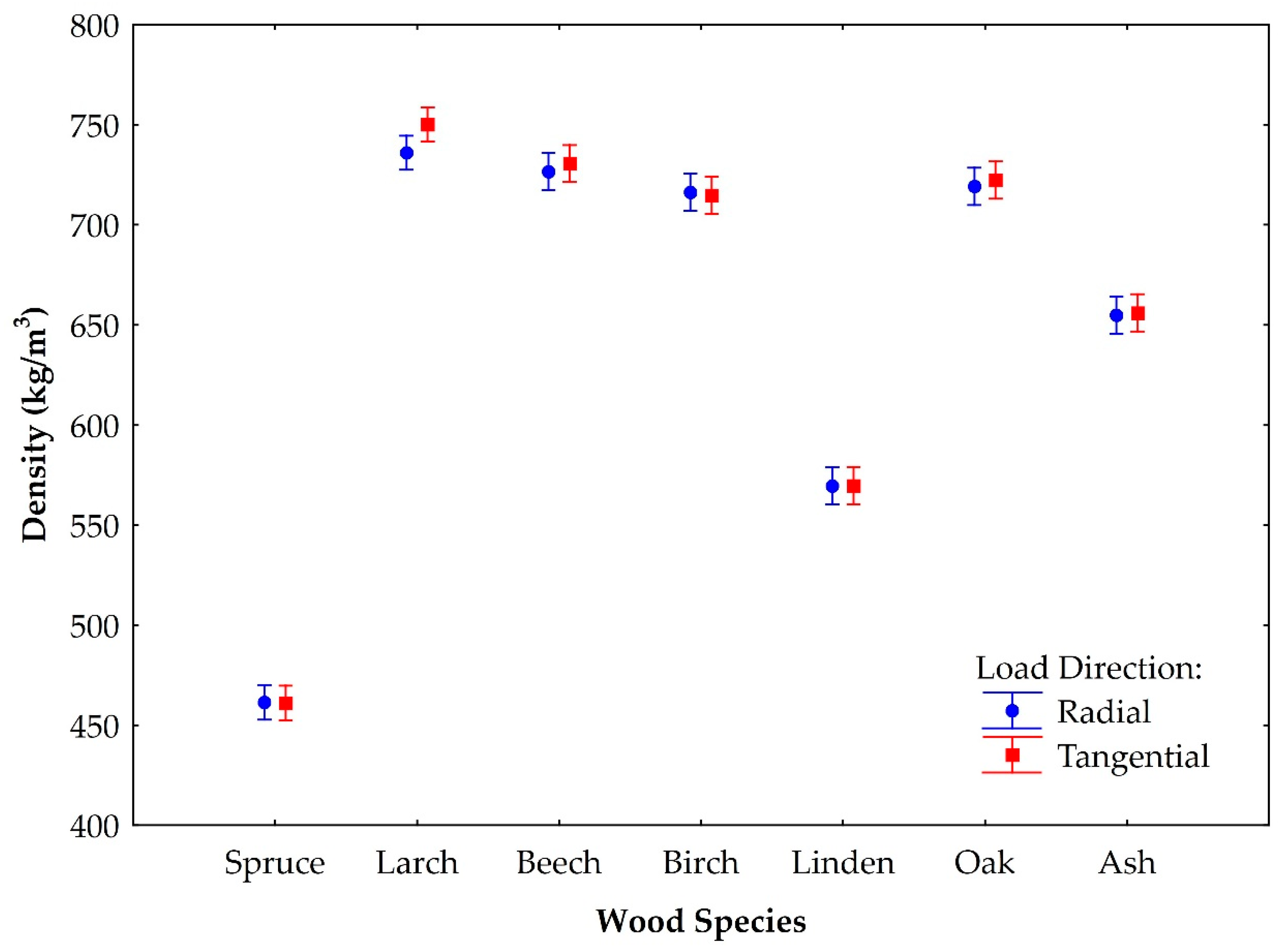
The wood density of individual wood species was determined after air-conditioning of the test specimens. After the air-conditioning, absolute moisture was ascertained for the individual woods, namely 13.8% for spruce wood, 13.3% for larch, 11.9% for beech, 11.7% for birch, 10.2% for linden, 11.5% for oak and 12.0% for ash. The graph (Figure 4) shows the determined values of wood density for individual examined wood species. The highest average density was recorded for larch wood, i.e., 760 kg/m³ for samples that were tested under loading in the tangential direction. The lowest density was recorded for spruce wood, for which the same average density was found for both sets of samples (radial and tangential direction of loading), i.e., 463 kg/m³. Statistically significant differences in mean values depending on the direction of loading were demonstrated for larch wood, and Duncan’s test (

Table A3. Duncan´s Multiple Range Test for Density.

MS = 1792.1

Sp

Sp

La

La

Be

Be

Bi

Bi

Li

Li

Oa

Oa

As

As

DF = 1106

Rd

Tg

Rd

Tg

Rd

Tg

Rd

Tg

Rd

Tg

Rd

Tg

Rd

Tg

Sp

Rd

Sp

Tg

0.976

La

Rd

0.000 *

0.000 *

La

Tg

0.000 *

0.000 *

0.031 *

Be

Rd

0.000 *

0.000 *

0.180

0.001 *

Be

Tg

0.000 *

0.000 *

0.415

0.004 *

0.541

Bi

Rd

0.000 *

0.000 *

0.006 *

0.000 *

0.153

0.050

Bi

Tg

0.000 *

0.000 *

0.003 *

0.000 *

0.107

0.031 *

0.812

Li

Rd

0.000 *

0.000 *

0.000 *

0.000 *

0.000 *

0.000 *

0.000 *

0.000 *

Li

Tg

0.000 *

0.000 *

0.000 *

0.000 *

0.000 *

0.000 *

0.000 *

0.000 *

0.981

Oa

Rd

0.000 *

0.000 *

0.020 *

0.000 *

0.289

0.113

0.656

0.523

0.000 *

0.000 *

Oa

Tg

0.000 *

0.000 *

0.057

0.000 *

0.518

0.238

0.385

0.293

0.000 *

0.000 *

0.628

As

Rd

0.000 *

0.000 *

0.000 *

0.000 *

0.000 *

0.000 *

0.000 *

0.000 *

0.000 *

0.000 *

0.000 *

0.000 *

As

Tg

0.000 *

0.000 *

0.000 *

0.000 *

0.000 *

0.000 *

0.000 *

0.000 *

0.000 *

0.000 *

0.000 *

0.000 *

0.864

* Values are significant at p < 0.05. Error: between MS = mean squares, DF = degrees of freedom. Wood Species: Sp = Spruce; La = Larch; Be = Beech; Bi = Birch; Li = Linden; Oa = Oak; As = Ash. Load Direction: Rd = Radial; Tg = Tangential.

) was used for multiple comparisons. Wood density is highly variable and depends on many factors [5,14]. This claim is evident in the case of larch density, which appears to be nonstandard compared to the values specified, for example, by Tsoumis [5] or Wageführ [33]. Other determined densities of individual wood species coincide with the range of densities reported in the literature [5,33,34], except for oak wood, in which a slightly higher density was found, i.e., 719 or 722 kg/m³.

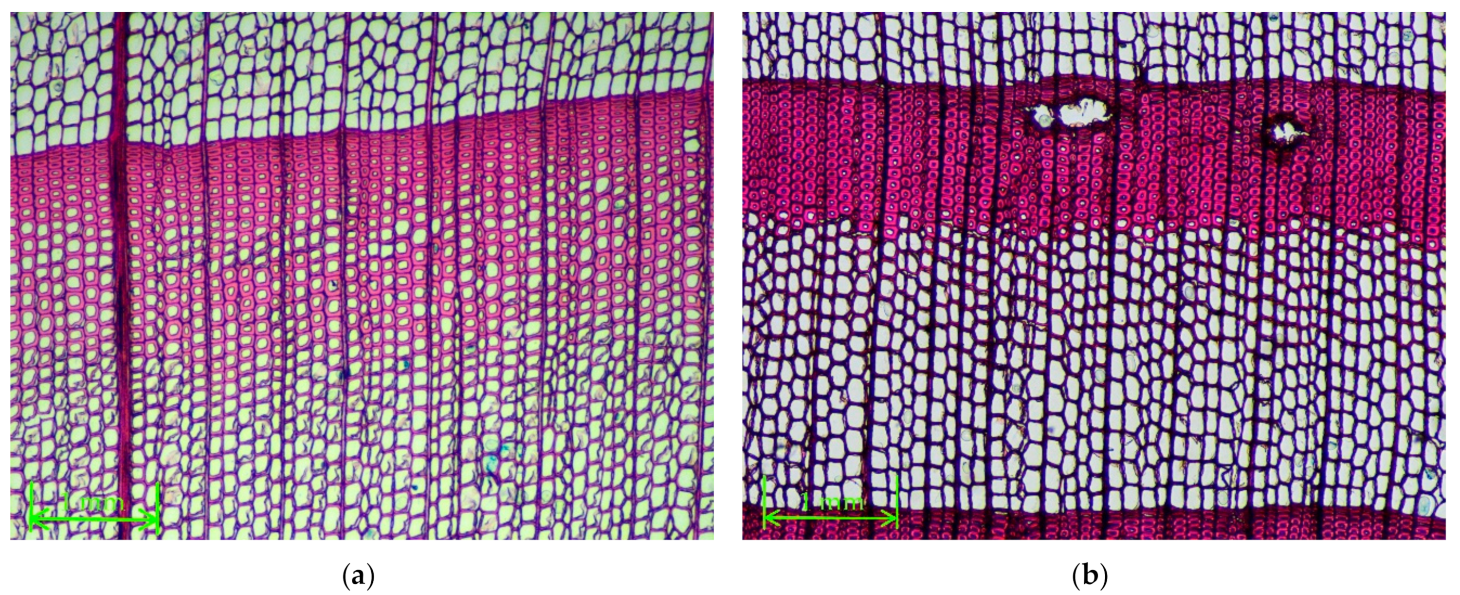
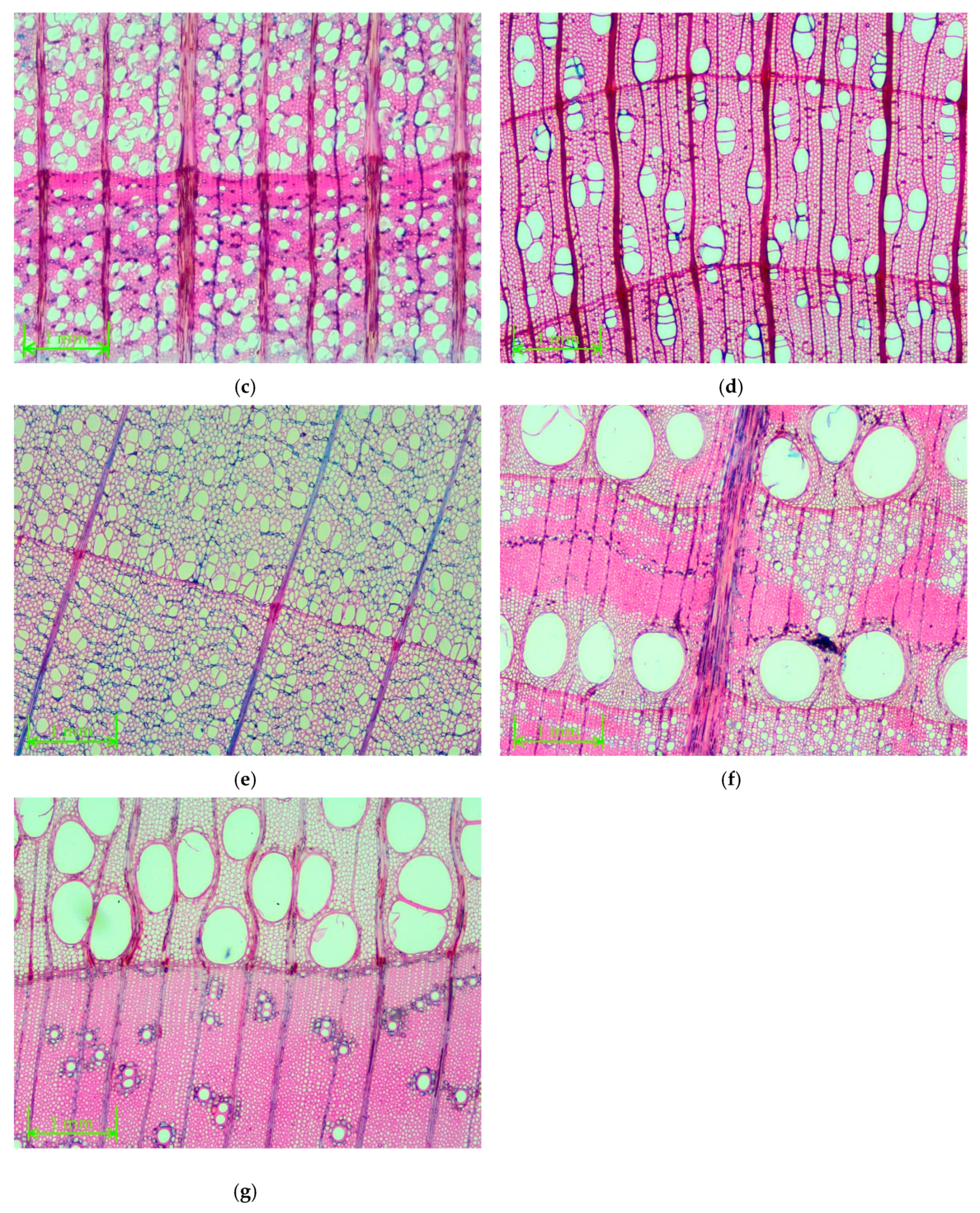
Table 1, Table 2, Table 3, Table 4, Table 5, Table 6 and Table 7 show the average widths of annual rings for individual wood species. The width and structure of the annual rings is highly variable and influenced by a large number of factors. The width of the annual ring changes both along the diameter of the trunk and along its length [3,5]. The largest width of the annual rings was found for ash wood, i.e., 2.9 mm, and the lowest for larch wood, 1.5 mm, which also showed the highest degree of variability. For birch wood with an average annual ring width of 2.4 mm, a nonstandard factor in the structure of annual rings was found after image analysis. The annual rings were markedly wavy in the cross section (Figure 5d). Figure 5 also shows examples of cross sections of wood of other wood species. All of the images are at 40× magnification.

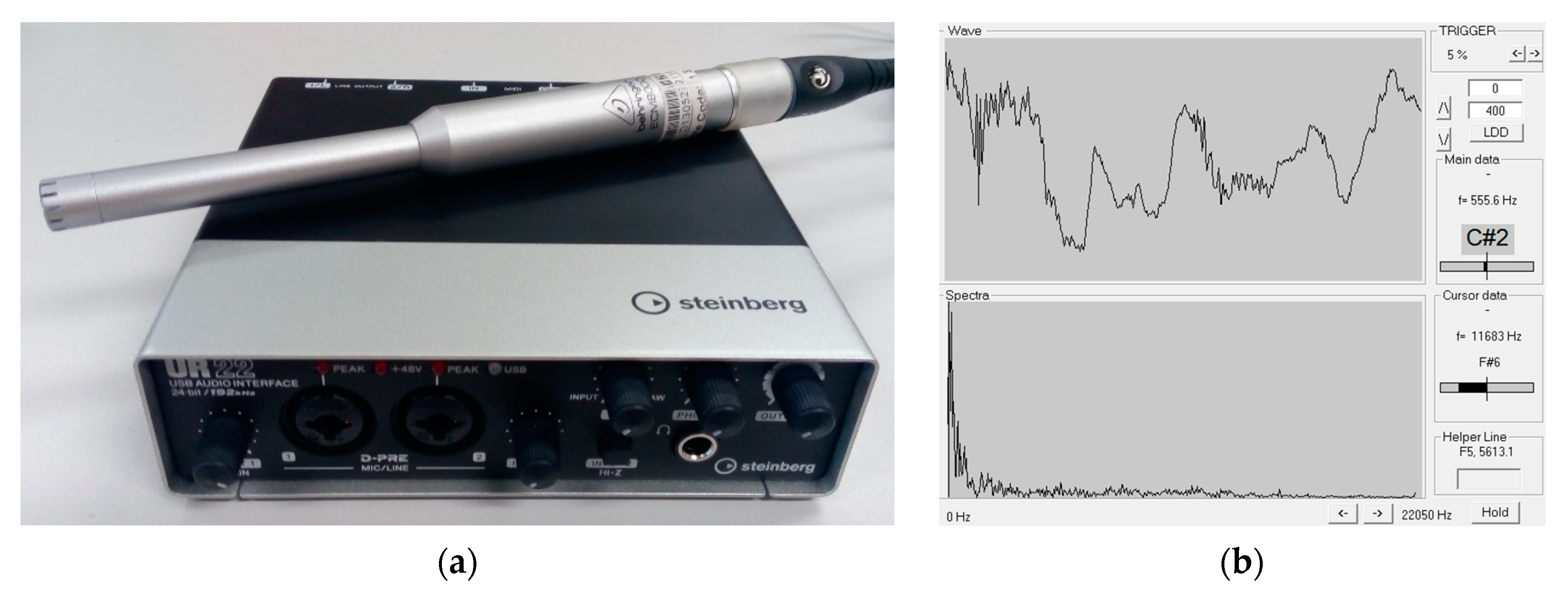
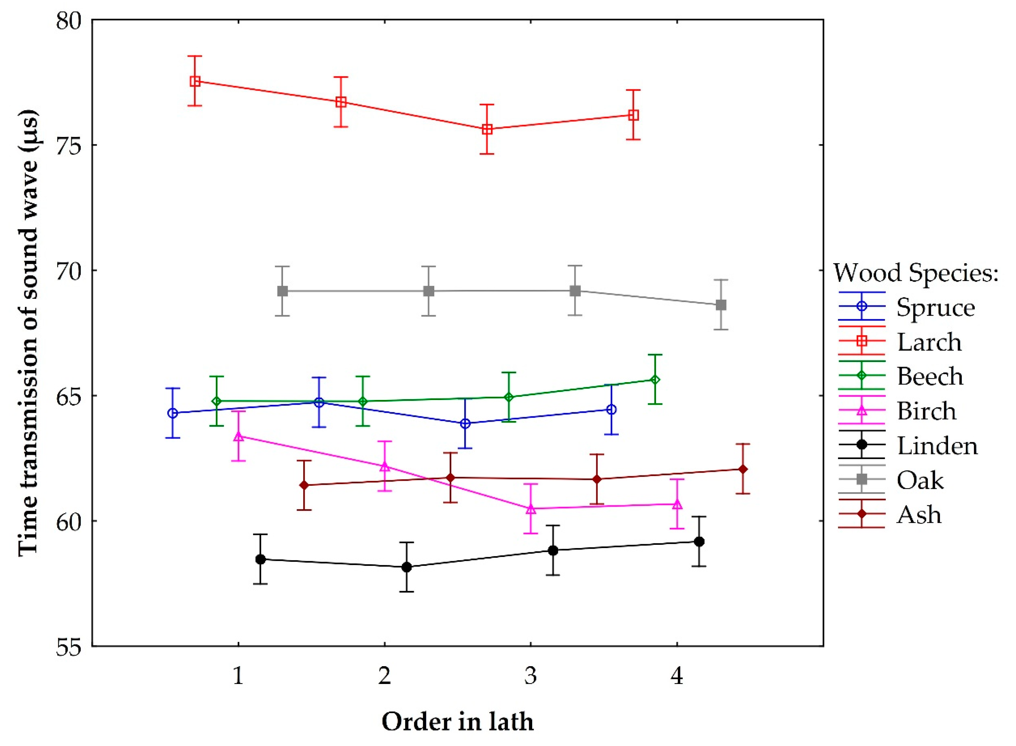
Dinwoodie [2] states in his work that bending strength is highly influenced by the occurrence of defects and the deviation of wood fibers from the longitudinal axis. However, in this work, great emphasis was placed on the quality of the tested material and the relative “homogeneity” of the test specimens was verified, which guaranteed the highest possible representative values of the investigated properties. This homogeneity was verified by the ultrasound and resonance methods. For clarity, the resonance method (Figure 6) is specified, which monitored the time of passage of the sound wave in the test specimens on the basis of the tests they were subjected to. The measured time should be almost identical or similar without significant statistical differences. Only under this assumption were the errors eliminated, and the obtained values determining any of the properties had a more representative weight. After evaluating the data, the differences between the test samples, which followed each other within a specific test, were primarily monitored. Thus, in order to determine the static bending strength, the first two test samples in the lath (1 and 2) were compared, and to determine the dynamic strength (impact strength), the following test specimens, i.e., 3 and 4, were compared. It can be seen from the specified graph that this assumption was fulfilled, and the samples did not show any significant differences amongst themselves. A significant difference was observed for birch wood between samples 1 and 2, i.e., for wood samples in which annual ring corrugation was observed (Figure 5d).

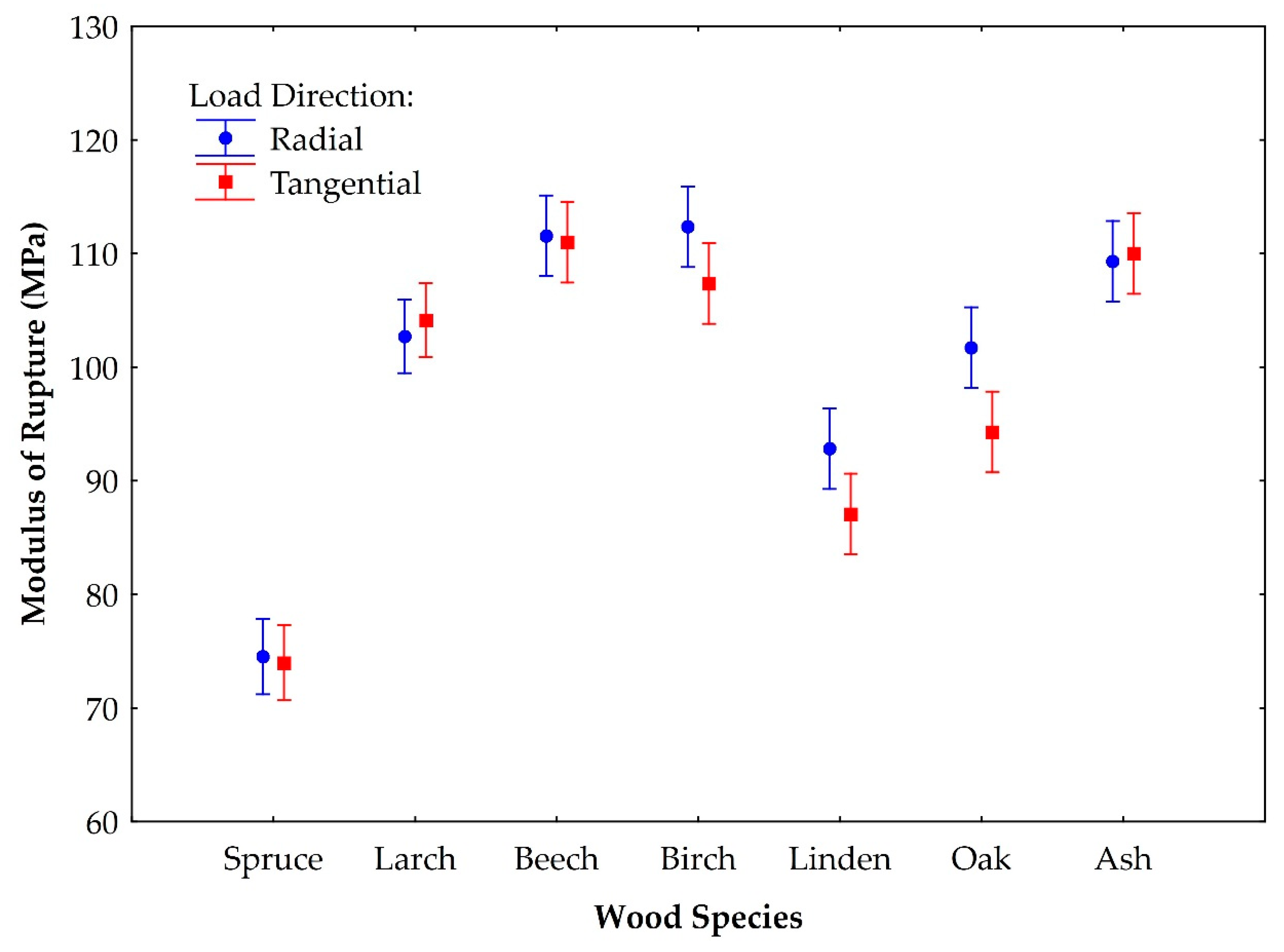
It is clear from the graphical representation (Figure 7) that the highest values of static bending strength were achieved by birch wood when loading test specimens in the radial direction. The mean value of the bending strength limit in this case was 112.4 MPa. The lowest mean value was achieved by spruce wood under load in the radial direction, i.e., 87.1 MPa. Larch, beech and ash wood showed similar average values of static bending strength in both loading directions, i.e., in the range of 104.6 to 111.6 MPa. The mean value of bending strength for oak wood was 94.3 MPa in the tangential direction and 101.7 MPa in the radial direction of the load. All of the detected values of static bending strength for the selected wood species under load in the radial or tangential direction are given above in Table 1, Table 2, Table 3, Table 4, Table 5, Table 6 and Table 7. It is clear from the above tables that the highest degree of variability in the values of the bending strength limit was shown by oak wood, and the lowest degree of variability was observed in ash wood, in both directions. Figure 7 also shows that the largest differences in the mean values of bending strength between the directions were achieved by oak wood, whilst lower differences were observed for linden and birch wood. Spruce, larch, beech and ash wood showed almost no differences in static bending strength values depending on the direction of the test specimen load.

Some authors state [6,13] that the ultimate strength of tangential bending can be 10% to 12% higher than that of radial bending in the wood of coniferous trees (softwoods). Požgaj et al. [6] state in their work that for deciduous wood species (hardwoods), these differences in static bending are negligible in the range of 2% to 4%.

Table 8 shows the differences in the mean values of static bending strength for wood of selected wood species depending on the direction of loading. These differences are expressed as a percentage and are related to how the mean values of static bending strength at radial load have changed from the values found in the tangential direction. The table shows that the largest difference was recorded for oak wood, i.e., 7.9%, while minor differences were found for linden wood, 6.6%, and birch, 4.7%, and for spruce, larch, beech and ash wood, these differences are negligible. Statistically significant differences in mean values between loading directions were demonstrated for oak and linden wood, and Duncan’s test was used for multiple comparisons (see Appendix A

Table A1. Duncan’s Multiple Range Test for Modulus of Rupture.

MS = 130.62

Sp

Sp

La

La

Be

Be

Bi

Bi

Li

Li

Oa

Oa

As

As

DF = 546

Rd

Tg

Rd

Tg

Rd

Tg

Rd

Tg

Rd

Tg

Rd

Tg

Rd

Tg

Sp

Rd

Sp

Tg

0.829

La

Rd

0.000 *

0.000 *

La

Tg

0.000 *

0.000 *

0.566

Be

Rd

0.000 *

0.000 *

0.001 *

0.007 *

Be

Tg

0.000 *

0.000 *

0.002 *

0.012 *

0.823

Bi

Rd

0.000 *

0.000 *

0.000 *

0.003 *

0.755

0.618

Bi

Tg

0.000 *

0.000 *

0.078

0.199

0.136

0.186

0.081

Li

Rd

0.000 *

0.000 *

0.000 *

0.000 *

0.000 *

0.000 *

0.000 *

0.000 *

Li

Tg

0.000 *

0.000 *

0.000 *

0.000 *

0.000 *

0.000 *

0.000 *

0.000 *

0.021 *

Oa

Rd

0.000 *

0.000 *

0.688

0.361

0.000 *

0.001 *

0.000 *

0.037 *

0.001 *

0.000 *

Oa

Tg

0.000 *

0.000 *

0.001 *

0.000 *

0.000 *

0.000 *

0.000 *

0.000 *

0.558

0.005 *

0.003 *

As

Rd

0.000 *

0.000 *

0.014 *

0.049 *

0.421

0.530

0.290

0.430

0.000 *

0.000 *

0.005 *

0.000 *

As

Tg

0.000 *

0.000 *

0.007 *

0.030 *

0.558

0.686

0.399

0.322

0.000 *

0.000 *

0.002 *

0.000 *

0.788

* Values are significant at p < 0.05. Error: between MS = mean squares, DF = degrees of freedom. Wood Species: Sp = Spruce; La = Larch; Be = Beech; Bi = Birch; Li = Linden; Oa = Oak; As = Ash. Load Direction: Rd = Radial; Tg = Tangential.

).

It is evident from the above that for woods of certain deciduous wood species (oak, linden), higher and statistically significant differences in mean values of the limit bending strength depending on the direction of loading were achieved than those reported by Požgaj et al. [6]. Despite this fact, these differences are considered negligible, and in their works, some authors [5,6,34] report only the values of static bending strength, which were obtained by standardized procedures, i.e., in the tangential direction.

The determined values of static bending strength under load in the tangential direction (Table 1, Table 2, Table 3, Table 4, Table 5, Table 6 and Table 7) for woods of selected wood species coincide with the range of values specified in [5,6,34], except for Linden wood, for which the mean value of the strength limit in static bending was significantly higher. Similarly, Pelit et al. [35] state in their work that their ascertained value of static bending strength for linden wood is 60.9 MPa, which is also significantly lower than the value determined in our research.

Table 1, Table 2, Table 3, Table 4, Table 5, Table 6 and Table 7 further show that the highest values of static modulus of elasticity were achieved by birch wood when loading test specimens in the radial direction. The mean value of the static modulus of elasticity in this case was 11,643 MPa. Linden wood achieved the lowest mean value under load in the tangential direction, i.e., 9332 MPa. Other mean values of the static modulus of elasticity depending on the direction of load in the investigated wood species obtained values between the maximum and minimum mean value given above. The highest degree of variability in the values of static modulus of elasticity was shown by oak wood, whilst the lowest degree of variability was observed in ash wood. In both cases, this variability was demonstrated in both the radial and tangential directions of loading. The determined values of the static modulus of elasticity had a similar trend depending on the direction of loading as in bending strength, except for ash wood, where the opposite trend was observed. The static modulus of elasticity values in the woods of the studied wood species are similar to those reported by some authors in their works [1,3,6]. The only exception is birch wood, for which lower values were found compared to the values reported by these authors.

For comparison, dynamic modules of elasticity are also specified in Table 1, Table 2, Table 3, Table 4, Table 5, Table 6 and Table 7. It turned out that in all of the methods, the highest mean values of dynamic modulus of elasticity were achieved by birch wood, i.e., in the range of 16,883 to 18,808 MPa. The lowest mean values were achieved by spruce wood in all of the methods, i.e., in the range of 7748 to 10,367 MPa. For larch wood, the greatest degree of variability was demonstrated using the ultrasound method (from the fronts), and for the remaining two methods, oak wood had the greatest degree of variability. Ash wood generally showed the lowest degree of variability. Furthermore, it is also evident that the highest mean values of the dynamic modulus of elasticity were achieved in almost all of the examined wood species using the ultrasound method, where piezoelectric sensors were applied to the sample surfaces, except for larch wood, where the opposite trend prevailed. The lowest mean values were achieved with the second ultrasound method (sensors were applied to the end faces of the samples), except for beech and larch wood. Dynamic modules determined via the resonance methods were slightly higher, except for spruce, larch and beech wood, where the opposite trend prevailed. In their work, Oberhofnerová et al. [21] determined the dynamic modulus of elasticity for spruce and oak wood via the ultrasound method (piezoelectric sensors were applied to the test specimen surfaces) and the resonance method, and there were similar differences between the mean values of the dynamic modulus of elasticity in oak wood as in this work. However, for spruce wood, such high differences were not recorded depending on the method used, as is also the case in this work. Holeček et al. [20] also found small differences in spruce wood depending on the method used. Based on these facts, it can be concluded that deciduous wood species have larger differences in the values of the dynamic modulus of elasticity depending on the method used than in coniferous trees. This can be explained by the fact that coniferous trees have a simpler anatomical structure than deciduous woods, and the propagation of the sound wave is to some extent influenced by this anatomical structure.

Compared to static modules of elasticity, dynamic modules of elasticity are largely overestimated. In the case of the examined coniferous tree wood, these differences were monitored up to 20%. For wood species with a scattered porous wood structure, these differences were more pronounced, i.e., in the range of 36% to 68%, and for wood species with a circularly porous structure in the range of 21% to 44%.

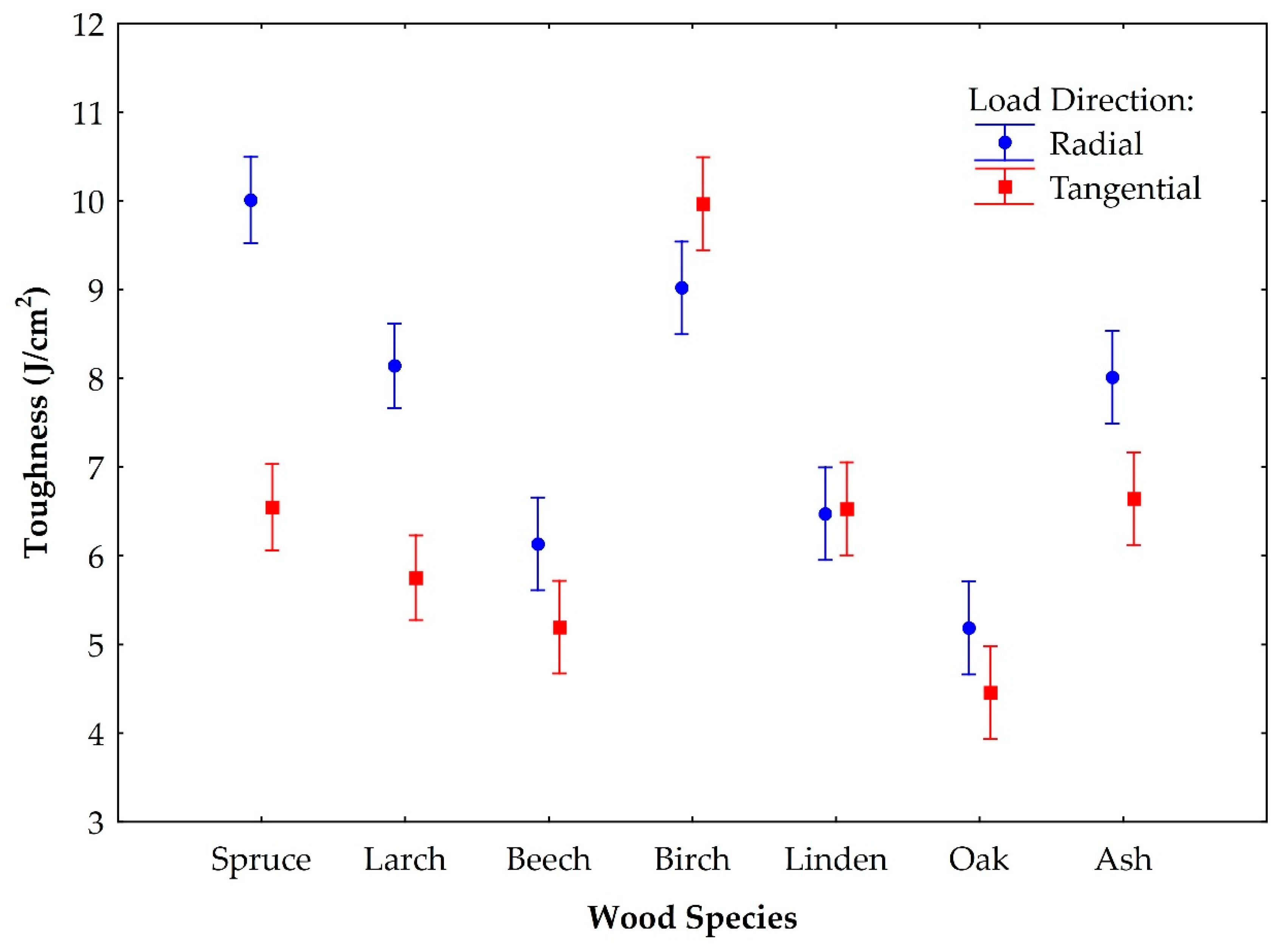
The graphical representation (Figure 8) shows that the highest values of impact (dynamic) strength were achieved by birch wood when loading test specimens in the tangential direction. The mean value of impact strength in this case was 10.0 J/cm². The lowest mean value was achieved by oak wood in the tangential direction i.e., 4.5 J/cm². For linden wood, almost no difference was observed in the average values of impact strength depending on the direction of loading, with a mean value of 6.5 J/cm². The largest differences in the average values of dynamic toughness were recorded for spruce wood, which were 9.8 J/cm² in the radial direction and 6.5 J/cm² in the loading tangential direction. All of the ascertained values are specified in Table 1, Table 2, Table 3, Table 4, Table 5, Table 6 and Table 7. It is clear from the above tables that the highest degree of variability in the values of dynamic toughness was shown by spruce wood under load in the radial direction and the lowest degree of variability was observed in ash wood, i.e., both in the loading tangential and radial direction. It was also found that the mean values of impact strength depend on both the type of wood species and the direction of loading of the test specimens. There were significant differences depending on the direction of loading in spruce wood, larch, beech, oak, birch and ash. In their work, Požgaj et al. [6] state that for wood with a significant difference between spring and summer wood, i.e., for coniferous and deciduous wood species with a circularly porous structure, the work consumed for rupturing the test specimen (impact strength) is higher, in the range of 25% to 50%, in the radial than in the tangential direction of loading. Požgaj et al. [6] did not notice any significant differences in the wood of deciduous wood species with a scattered porous wood structure. It is clear from Table 8 that this claim agrees for coniferous tree wood and wood species with a circularly porous wood structure, but this is not the case for scattered porous wood species. The table shows that the largest difference in mean values was recorded for spruce wood, i.e., 50.3%, and slightly smaller differences were observed for larch wood 41.2%. Smaller differences of about 20% were recorded for beech, ash and oak wood. For birch wood, a difference was recorded with the opposite trend than for the woods mentioned above, i.e., −9.5%. This peculiarity can be explained by the fact that despite careful selection of the material and verification of its relative “homogeneity”, it was found after image analysis that birch wood shows a significant, but slight ripple in the annual ring that cannot be seen with the human eye (Figure 5d). It can be concluded from this that this ripple greatly affected the impact strength values. Linden wood showed almost no difference, and this difference (−0.8%) can be considered negligible. Duncan’s test (

Table A2. Duncan’s Multiple Range Test for Toughness.

MS = 2.8329

Sp

Sp

La

La

Be

Be

Bi

Bi

Li

Li

Oa

Oa

As

As

DF = 546

Rd

Tg

Rd

Tg

Rd

Tg

Rd

Tg

Rd

Tg

Rd

Tg

Rd

Tg

Sp

Rd

Sp

Tg

0.000 *

La

Rd

0.000 *

0.000

La

Tg

0.000 *

0.053

0.000 *

Be

Rd

0.000 *

0.311

0.000 *

0.301

Be

Tg

0.000 *

0.001 *

0.000 *

0.130

0.015 *

Bi

Rd

0.010 *

0.000 *

0.017 *

0.000 *

0.000 *

0.000 *

Bi

Tg

0.910

0.000 *

0.000 *

0.000 *

0.000 *

0.000 *

0.010 *

Li

Rd

0.000 *

0.852

0.000 *

0.063

0.355

0.001 *

0.000 *

0.000 *

Li

Tg

0.000 *

0.959

0.000 *

0.053

0.315

0.001 *

0.000 *

0.000 *

0.882

Oa

Rd

0.000 *

0.001 *

0.000 *

0.147

0.017 *

0.982

0.000 *

0.000 *

0.001 *

0.001 *

Oa

Tg

0.000 *

0.000 *

0.000 *

0.001 *

0.000 *

0.058

0.000 *

0.000 *

0.000 *

0.000 *

0.048 *

As

Rd

0.000 *

0.000 *

0.729

0.000 *

0.000 *

0.000 *

0.009 *

0.000 *

0.000 *

0.000 *

0.000 *

0.000 *

As

Tg

0.000 *

0.793

0.000 *

0.032 *

0.223

0.000 *

0.000 *

0.000 *

0.680

0.770

0.000 *

0.000 *

0.000 *

* Values are significant at p < 0.05. Error: between MS = mean squares, DF = degrees of freedom. Wood Species: Sp = Spruce; La = Larch; Be = Beech; Bi = Birch; Li = Linden; Oa = Oak; As = Ash. Load Direction: Rd = Radial; Tg = Tangential.

) was used for multiple comparisons. Statistically significant differences in the mean values of impact strength depending on the direction of loading were demonstrated in spruce, larch, beech, birch, oak and ash wood, and in linden wood, no statistically significant difference was demonstrated.

Overall, it can be concluded that the impact strength values between the individual studied wood species and directions of loading are highly influenced by the anatomical structure of the wood of individual wood species and the percentage representation of basic building elements (vessels, tracheids, parenchymal cells, libriform fibers, etc.). Furthermore, it can be concluded that the anatomical structure and the percentage of individual building elements are more pronounced in the determination of dynamic toughness and contribute to the difference in values in the radial and tangential directions of loading than in the case of bending strength under static loading. The values will also be influenced both by the submicroscopic structure of wood (fibrillar structure) and by the representation of basic building biopolymers of wood (cellulose, hemicelluloses, lignin) in individual anatomical elements of wood. In their work, Conrad el. al. [36] addressed the results of several authors and came to the conclusion that in the case of wood failure, there is a different crack propagation at the microscopic and submicroscopic level of wood depending on the direction of loading, from which it can be deduced that different crack propagation in wood from various selected wood species will also affect the resulting dynamic toughness values. 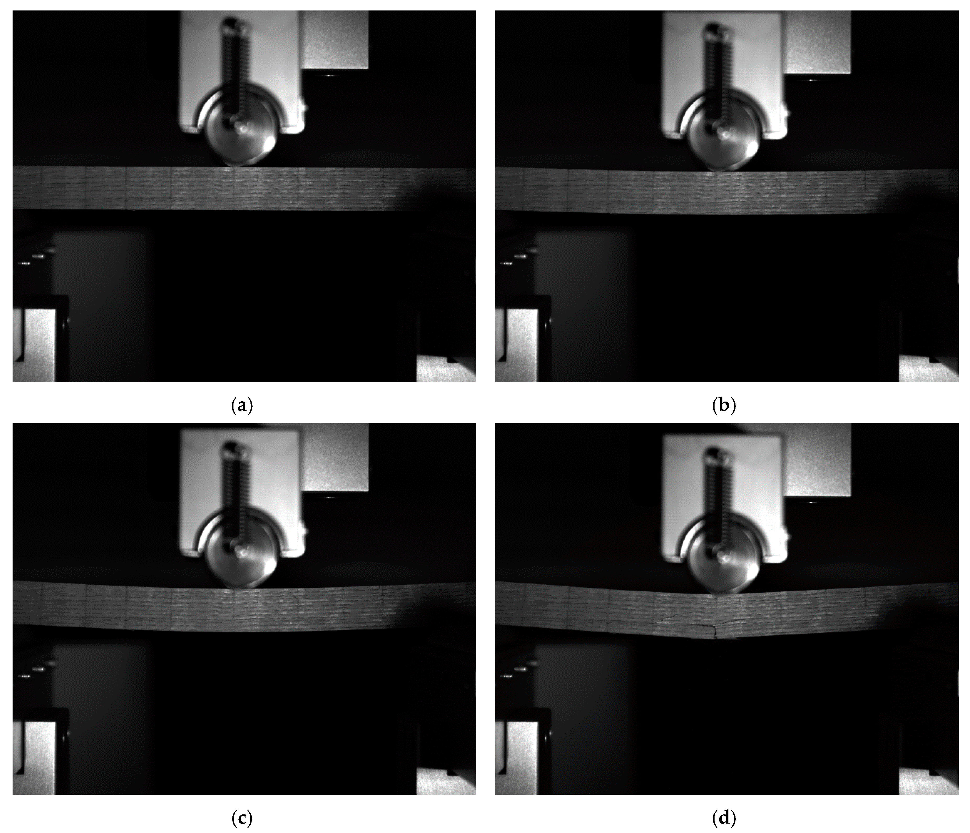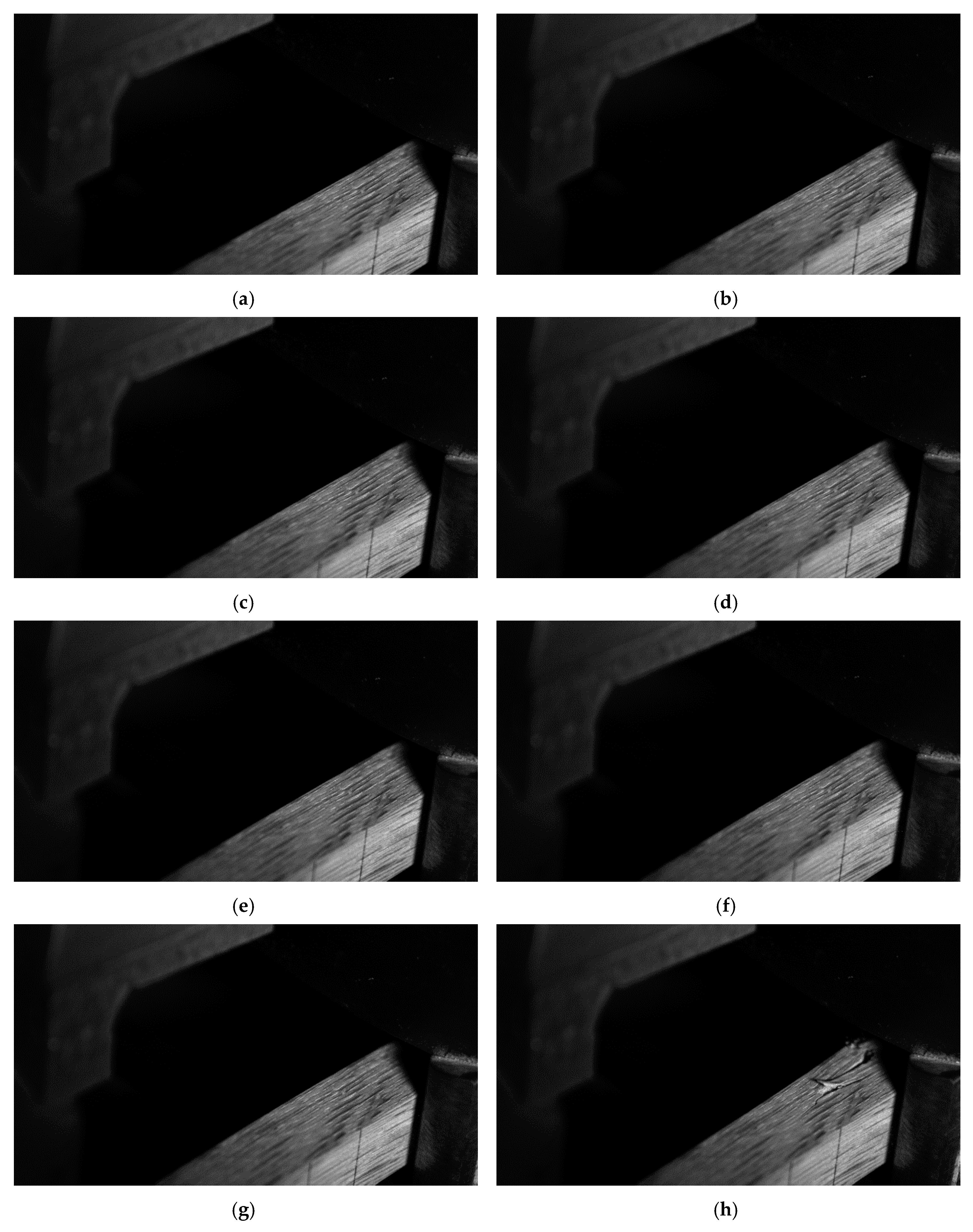The same can be assumed for static loads in bending (see Figure 9 and Figure 10). Furthermore, it can be concluded that with dynamic loading of wood in the radial direction, there is a higher resistance of the material, because the impact energy must alternately pass through the spring and summer wood, which does not occur with loading in the tangential direction.

It is clear that various methodologies can be used to determine the bending characteristics of wood, often using nondestructive principles, such as Near-Infrared Spectroscopy [37]. However, the standardized methodologies can be said to be, from a principle point of view and in compliance with the conditions of the experiments, still the most accurate methods, especially from the point of view of the validity of the obtained results.

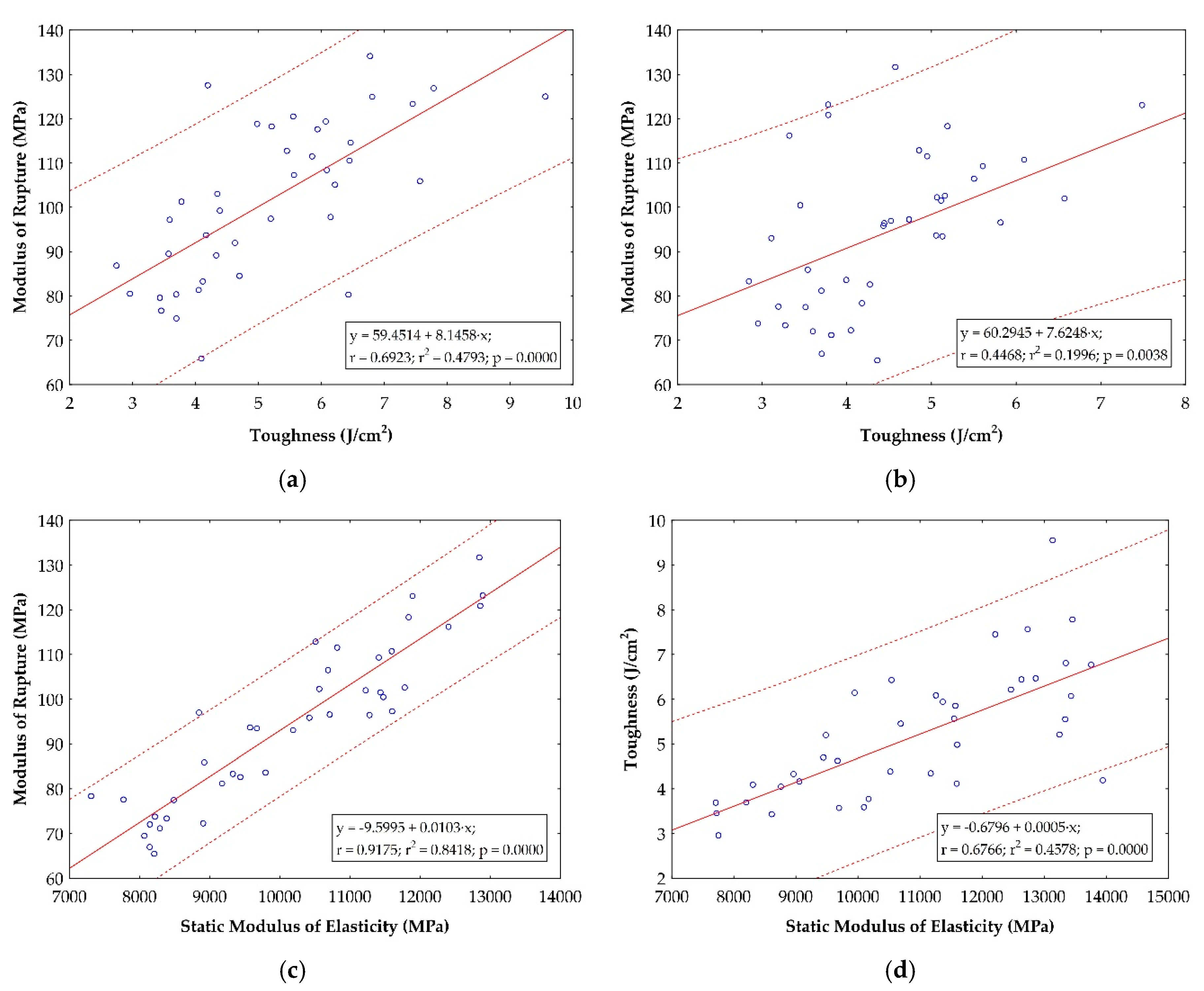
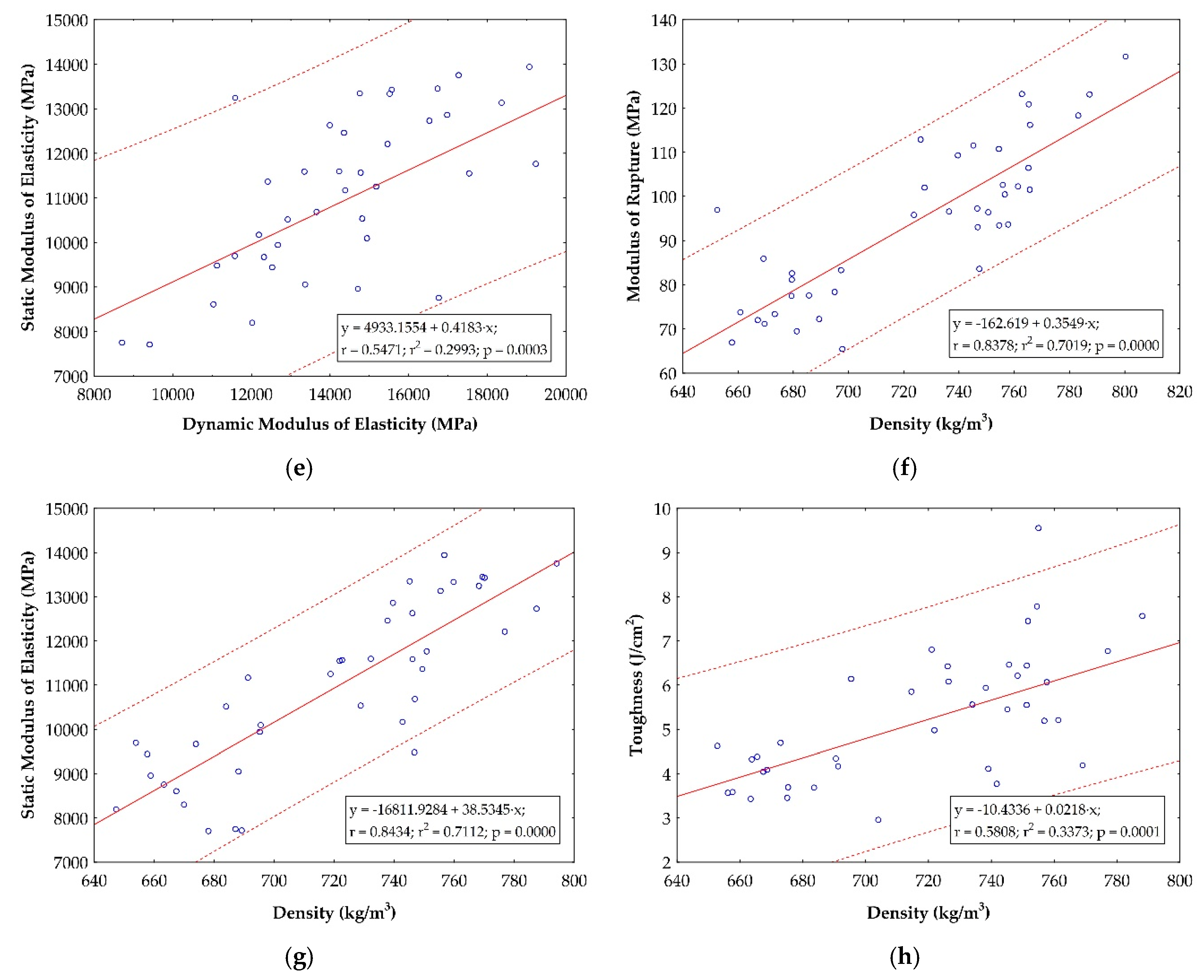
With regard to the investigated wood species, it is often possible to observe dependencies between the individual obtained quantities or properties. Based on this fact, correlation matrices were created (see

Table A4. Values of Correlation Coefficients Between Given Quantities for Spruce Wood.

		MOR		Toughness		Static MOE		Dynamic MOE *		Density
		Radial	Tangential	Radial	Tangential	Radial	Tangential	Radial	Tangential	Radial	Tangential
MOR	Radial
	Tangential	0.092
Toughness	Radial	0.429	−0.015
	Tangential	0.043	0.234	0.479
Static MOE	Radial	0.738	0.177	0.370	0.154
	Tangential	0.548	0.712	0.300	0.237	0.508
Dynamic MOE *	Radial	0.399	0.013	−0.050	0.294	0.470	0.371
	Tangential	0.420	0.209	0.227	0.190	0.367	0.522	0.466
Density	Radial	0.645	0.411	0.377	0.295	0.624	0.736	0.444	0.617
	Tangential	0.618	0.342	0.135	0.022	0.578	0.632	0.249	0.548	0.879

Red coloring = Significant at p < 0.05; MOR = Modulus of Rupture; MOE = Dynamic Modulus of Elasticity; * determined by the Ultrasound Method (from the side surface).

,

Table A5. Values of Correlation Coefficients Between Given Quantities for Larch Wood.

		MOR		Toughness		Static MOE		Dynamic MOE *		Density
		Radial	Tangential	Radial	Tangential	Radial	Tangential	Radial	Tangential	Radial	Tangential
MOR	Radial
	Tangential	0.471
Toughness	Radial	0.368	0.742
	Tangential	0.170	0.560	0.726
Static MOE	Radial	0.657	0.561	0.429	0.214
	Tangential	0.394	0.833	0.689	0.500	0.770
Dynamic MOE *	Radial	0.424	0.355	0.727	0.540	0.719	0.597
	Tangential	0.308	0.697	0.507	0.408	0.633	0.781	0.427
Density	Radial	0.475	0.516	0.337	0.175	0.417	0.361	0.082	0.385
	Tangential	0.428	0.623	0.319	0.183	0.355	0.410	0.001	0.425	0.912

Red coloring = Significant at p < 0.05; MOR = Modulus of Rupture; MOE = Dynamic Modulus of Elasticity; * determined by the Ultrasound Method (from the side surface).

,

Table A6. Values of Correlation Coefficients Between Given Quantities for Beech Wood.

		MOR		Toughness		Static MOE		Dynamic MOE *		Density
		Radial	Tangential	Radial	Tangential	Radial	Tangential	Radial	Tangential	Radial	Tangential
MOR	Radial
	Tangential	0.670
Toughness	Radial	0.390	0.319
	Tangential	0.197	0.155	0.019
Static MOE	Radial	0.867	0.591	0.478	0.219
	Tangential	0.616	0.638	0.323	0.547	0.745
Dynamic MOE *	Radial	0.586	0.453	0.312	0.299	0.482	0.584
	Tangential	0.147	0.156	0.152	0.413	0.134	0.324	0.322
Density	Radial	0.110	0.204	0.315	0.066	0.189	0.192	0.119	−0.051
	Tangential	0.498	0.515	0.221	−0.047	0.508	0.517	0.435	0.055	0.799

Red coloring = Significant at p < 0.05; MOR = Modulus of Rupture; MOE = Dynamic Modulus of Elasticity; * determined by the Ultrasound Method (from the side surface).

,

Table A7. Values of Correlation Coefficients Between Given Quantities for Birch Wood.

		MOR		Toughness		Static MOE		Dynamic MOE *		Density
		Radial	Tangential	Radial	Tangential	Radial	Tangential	Radial	Tangential	Radial	Tangential
MOR	Radial
	Tangential	−0.038
Toughness	Radial	−0.351	−0.019
	Tangential	−0.468	0.346	0.548
Static MOE	Radial	0.874	0.059	−0.483	−0.554
	Tangential	0.170	0.773	−0.161	0.138	0.376
Dynamic MOE *	Radial	0.635	0.015	−0.095	−0.150	0.714	0.267
	Tangential	0.295	0.057	−0.295	−0.021	0.459	0.341	0.300
Density	Radial	0.002	0.458	0.594	0.530	0.149	0.636	0.083	0.044
	Tangential	−0.069	0.369	0.550	0.654	−0.031	0.487	0.034	−0.022	0.753

Red coloring = Significant at p < 0.05; MOR = Modulus of Rupture; MOE = Dynamic Modulus of Elasticity; * determined by the Ultrasound Method (from the side surface).

,

Table A8. Values of Correlation Coefficients Between Given Quantities for Linden Wood.

		MOR		Toughness		Static MOE		Dynamic MOE *		Density
		Radial	Tangential	Radial	Tangential	Radial	Tangential	Radial	Tangential	Radial	Tangential
MOR	Radial
	Tangential	0.198
Toughness	Radial	0.093	0.054
	Tangential	−0.061	0.191	0.128
Static MOE	Radial	0.842	0.266	0.043	0.153
	Tangential	0.070	0.926	−0.016	0.233	0.199
Dynamic MOE *	Radial	0.513	0.451	0.451	0.265	0.639	0.505
	Tangential	0.108	0.546	0.107	0.120	0.285	0.646	0.552
Density	Radial	0.429	0.560	0.191	−0.016	0.494	0.641	0.541	0.510
	Tangential	0.177	0.646	0.051	0.057	0.370	0.763	0.422	0.498	0.878

Red coloring = Significant at p < 0.05; MOR = Modulus of Rupture; MOE = Dynamic Modulus of Elasticity; * determined by the Ultrasound Method (from the side surface).

,

Table A9. Values of Correlation Coefficients Between Given Quantities for Oak Wood.

		MOR		Toughness		Static MOE		Dynamic MOE *		Density
		Radial	Tangential	Radial	Tangential	Radial	Tangential	Radial	Tangential	Radial	Tangential
MOR	Radial
	Tangential	0.708
Toughness	Radial	0.692	0.680
	Tangential	0.305	0.447	0.509
Static MOE	Radial	0.874	0.754	0.677	0.342
	Tangential	0.812	0.918	0.726	0.390	0.916
Dynamic MOE *	Radial	0.388	0.423	0.314	0.159	0.547	0.539
	Tangential	0.409	0.442	0.073	0.207	0.487	0.504	0.800
Density	Radial	0.775	0.845	0.581	0.513	0.843	0.882	0.429	0.405
	Tangential	0.791	0.838	0.519	0.549	0.816	0.866	0.379	0.360	0.979

Red coloring = Significant at p < 0.05; MOR = Modulus of Rupture; MOE = Dynamic Modulus of Elasticity; * determined by the Ultrasound Method (from the side surface).

and

Table A10. Values of Correlation Coefficients Between Given Quantities for Ash Wood.

		MOR		Toughness		Static MOE		Dynamic MOE *		Density
		Radial	Tangential	Radial	Tangential	Radial	Tangential	Radial	Tangential	Radial	Tangential
MOR	Radial
	Tangential	0.388
Toughness	Radial	0.170	0.032
	Tangential	0.130	0.054	0.295
Static MOE	Radial	0.670	0.532	0.311	0.132
	Tangential	0.455	0.663	0.375	0.318	0.755
Dynamic MOE *	Radial	0.022	0.317	0.371	0.003	0.345	0.307
	Tangential	0.029	0.337	0.088	0.163	0.455	0.430	0.334
Density	Radial	0.509	0.550	0.254	0.339	0.823	0.734	0.337	0.389
	Tangential	0.602	0.646	0.169	0.188	0.845	0.747	0.265	0.373	0.938

Red coloring = Significant at p < 0.05; MOR = Modulus of Rupture; MOE = Dynamic Modulus of Elasticity; * determined by the Ultrasound Method (from the side surface).

), by means of which the obtained quantities of wood of individual wood species were compared and, if possible, also depending on the direction of loading. As an example, some of the correlations were converted to graphical form (linear regression, see Figure 11). From the above graphs and tables, it is clear that relatively strong dependencies were observed between some variables, i.e., in particular in the case of oak wood, where dependence was proven in almost all cases. Dependence was not proven between impact toughness (tangential direction) and bending strength (radial direction), which is of course one of the dependencies without any significant justification. Furthermore, the dependence between impact strength and the dynamic modulus of elasticity was not demonstrated for oak wood. In this case, a statistically significant dependence was demonstrated only between the impact strength (radial direction) and the dynamic modulus of elasticity (radial direction) with a correlation coefficient of r = 0.314. In all other cases, statistically significant dependencies were demonstrated, with higher correlation coefficients than in the previous case. It is evident from the graphical expression (Figure 11a,b) that a medium–strong dependence (r ≅ 0.50 ÷ 0.75) was demonstrated between bending strength and impact strength, as well as between impact strength and static modulus of elasticity (Figure 11d). Similar statistically significant dependencies were also observed in oak wood in other cases. Very strong dependences (r > 0.75) were demonstrated between bending strength and static modulus of elasticity (Figure 11c), between bending strength and density (Figure 11f) and between the static modulus of elasticity and density (Figure 11g), as shown, for example, by Dinwoodie [2]. All of the other investigated dependencies, both for oak and the wood of other investigated wood species, are specified in Table A4, Table A5, Table A6, Table A7, Table A8, Table A9 and Table A10.

4. Conclusions

The following are the most important findings of this research focused on static and dynamic bending characteristics:

• The largest difference of mean values in impact bending strength in the radial direction toward tangential was recorded for spruce wood, i.e., 50.3%. Slightly smaller differences were observed for larch wood, i.e., 41.2%. Smaller differences of about 20% were recorded for beech, ash and oak wood. For birch wood, a difference was recorded with the opposite trend to the woods mentioned above, i.e., −9.5%. Linden wood showed almost no difference (−0.8%). The highest values of impact strength were achieved by birch wood when loading the test specimens in the tangential direction and spruce wood in the radial direction (approximately 10 J/cm²). The lowest values were achieved by oak wood in the tangential direction, on average 4.5 J/cm², and only slightly higher values in the radial direction.
• For static bending strength, it was found that the largest difference (radial/tangential) was recorded for oak wood, i.e., 7.9%, while minor differences were found for linden wood of 6.6% and birch of 4.7%. For spruce, larch, beech and ash wood, these differences are negligible. The highest values of static bending strength were achieved by birch wood when loading the test specimens in the radial direction (112.4 MPa). The lowest values were achieved by spruce wood under load in the radial direction—on average 87.1 MPa.
• Compared to static modules of elasticity, dynamic modules of elasticity are largely overestimated. In the case of the examined coniferous trees, these differences were up to a maximum of 20%. For wood species with a diffuse-porous wood structure, these differences were more pronounced, i.e., in the range of 36% to 68%, and for wood species with a ring-porous structure in the range of 21% to 43%. Regardless of the methods, in real terms, birch wood achieved the highest values of modulus of elasticity, whilst ash wood was slightly lower. The lowest values of modulus of elasticity were shown by spruce wood.
• It is evident from the correlation dependences between the individual quantities that most of them are statistically significant, especially in the case of oak wood, where dependence was proven in almost all cases. Very strong dependences were demonstrated between bending strength and static modulus of elasticity, between bending strength and density, as well as between static modulus of elasticity and density. It is also evident that a moderate dependence was demonstrated between bending strength and impact strength, as well as between impact strength and static modulus of elasticity, which are dependencies that are not normally monitored.

This paper is primarily intended to lead to a targeted expansion of the database dealing with bending characteristics, and thus help to understand the static and dynamic bending strength depending on the direction of the effects of external forces. Wood is very often used in structural elements of buildings; wood products (e.g., furniture), in which there is both a static load; and in many cases a dynamic load, while the direction of loading is usually not considered.

References

1. Bodig, J.; Jayne, B.A. Mechanics of Wood and Wood Composites, 1st ed.; Van Nostrand Reinhold: New York, NY, USA, 1982; p. 712. ISBN 0442008228. [Google Scholar]
2. Dinwoodie, J.M. Timber: Its Nature and Behavior, 2nd ed.; CRC Press: New York, NY, USA, 2000; p. 272. ISBN 978-0419235804. [Google Scholar]
3. Kollmann, F.F.P.; Côté, W.A. Principles of Wood Science and Technology–I Solid Wood; Springer: Berlin/Heidelberg, Germany, 1968; p. 592. ISBN 978-3-642-87930-2. [Google Scholar]
4. Shmulsky, R.; Jones, P.D. Forest Products and Wood Science An. Introduction, 6th ed.; Wiley: Hoboken, NJ, USA, 2011; p. 496. ISBN 978-0813820743. [Google Scholar]
5. Tsoumis, G.T. Science and Technology of Wood–Structure, Properties, Utilization, 1st ed.; Van Nostrand Reinhold: New York, NY, USA, 1991; p. 494. ISBN 9780442239855. [Google Scholar]
6. Požgaj, A.; Chovanec, D.; Kurjatko, S.; Babiak, M. Štruktúra a Vlastnosti Dreva (Structure and Properties of Wood), 1st ed.; Príroda: Bratislava, Slovakia, 1993; p. 485. ISBN 80-07-00600-1. [Google Scholar]
7. Madsen, B.; Nielsen, L.F. Structural Behaviour of Timber, 1st ed.; American Society of Civil Engineers: Reston, VA, USA, 1995; p. 405. ISBN 978-0969616207. [Google Scholar]
8. Borgström, E. (Ed.) Design of Timber Structures: Structural Aspects of Timber Construction Volume 1; Swedish Wood: Stockholm, Sweden, 2015; p. 314. ISBN 978-91-980304-8-8. [Google Scholar]
9. Breyer, D.E.; Fridley, K.J.; Pollock, D.G.; Cobeen, K.E. Design of Wood Structures—ASD/LRFD, 6th ed.; McGraw-Hill: New York, NY, USA, 2007; p. 1096. ISBN 978-0-07-145539-8. [Google Scholar]
10. Porteous, J.; Kermani, A. Structural Timber Design to Eurocode 5, 1st ed.; Blackwell Publishing: Malden, MA, USA, 2007; p. 452. ISBN 978-14051-4638-8. [Google Scholar]
11. Schober, K.U. (Ed.) Experimental Research with Timber; University of Bath: Bath, UK, 2014; p. 232. ISBN 1-85790-183-5. [Google Scholar]
12. Jansson, B. Impact Loading of Timber Beams. Ph.D. Thesis, The University of British Columbia, Vancouver, BC, Canada, 1992. [Google Scholar]
13. Güray, E.; Kasal, A.; Demirci, S.; Ceylan, E.; Kuşkun, T. Effects of cross-sectional geometry and force direction on bending strength and modulus of elasticity of some softwood beams. BioResources 2019, 14, 9258–9270. [Google Scholar] [CrossRef]
14. Zobel, B.J.; Buijtenen, J.P. Wood Variation: Its Causes and Control, 1st ed.; Springer: Berlin/Heidelberg, Germany, 1989; p. 363. ISBN 978-3-642-74071-8. [Google Scholar]
15. Beall, F. Overview of the use of ultrasonic technologies in research on wood properties. Wood Sci. Technol. 2002, 36, 197–212. [Google Scholar] [CrossRef]
16. Bucur, V. Acoustics of Wood, 2nd ed.; Springer: Berlin/Heidelberg, Germany, 2006; p. 394. ISBN 978-3-540-26123-0. [Google Scholar]
17. Kuttruff, H. Acoustics. An introduction; Taylor & Francis: New York, NY, USA, 2007; p. 457. ISBN 0-203-97089-6. [Google Scholar]
18. Bucur, V. Nondestructive Characterization and Imaging of Wood, 1st ed.; Springer: Berlin/Heidelberg, Germany, 2003; p. 354. ISBN 978-3-540-43840-3. [Google Scholar]
19. Reinprecht, L. Wood Deterioration, Protection and Maintenance, 1st ed.; John Wiley & Sons: Oxford, UK, 2016; p. 376. ISBN 978-1119106531. [Google Scholar]
20. Holeček, T.; Gašparík, M.; Lagaňa, R.; Borůvka, V.; Oberhofnerová, E. Measuring the modulus of elasticity of thermally treated spruce wood using the ultrasound and resonance methods. BioResources 2017, 12, 819–838. [Google Scholar] [CrossRef]
21. Oberhofnerová, E.; Arnetová, K.; Holeček, T.; Borůvka, V.; Bomba, J. Determination of Correlation between Destructive and Nondestructive Methods Applied on Modified Wood Exposed to Natural Weathering Test. BioResources 2016, 11, 5155–5168. [Google Scholar] [CrossRef]
22. ČSN 49 0101. Drevo. Všeobecné Požiadavky na Fyzikálne a Mechanické Skúšky (Wood. General Requirements for Physical and Mechanical Testing); Office for Standardization and Measurement: Prague, Czech Republic, 1 January 1980. [Google Scholar]
23. ČSN 49 0108. Drevo. Zisťovanie hustoty (Wood. Determination of the density); Czech Standards Institute: Prague, Czech Republic, 1 March 1993. [Google Scholar]
24. ČSN 49 0103. Drevo. Zisťovanie Vlhkosti pri Fyzikálnych a Mechanických Skúškach (Wood. Determination of Moisture Content at Physical and Mechanical Testing); Office for Standardization and Measurement: Prague, Czech Republic, 1 December 1979. [Google Scholar]
25. FAKOPP Ultrasonic Timer User’s Guide. Available online: http://fakopp.com/docs/products/ultrasonic/UltrasonicGuide.pdf (accessed on 1 July 2020).
26. ČSN 49 0115. Drevo. Zist’ovanie Medze Pevnosti v Statickom Ohybe (Wood. Determination of Ultimate Strength in Flexure Tests); Office for Standardization and Measurement: Prague, Czech Republic, 1 December 1979. [Google Scholar]
27. ČSN EN 310. Desky ze Dřeva. Stanovení Modulu Pružnosti v Ohybu a Pevnosti v Ohybu (Wood Based Panels. Determination of Modulus of Elasticity in Bending and of Bending Strength); Czech Standards Institute: Prague, Czech Republic, 1 January 1996. [Google Scholar]
28. ČSN 49 0116. Drevo. Metóda Zisťovania Modulu Pružnosti pri Statickom Ohybe (Wood. Determination of the Modulus of Elasticity in Static Bending); Office for Standardization and Measurement: Prague, Czech Republic, 1 January 1982. [Google Scholar]
29. ČSN 49 0117. Drevo. Rázová Húževnatosť v Ohybe (Wood. Impact Strength in Flexure); Office for Standardization and Measurement: Prague, Czech Republic, 1 January 1980. [Google Scholar]
30. Gärtner, H.; Lucchinetti, S.; Schweingruber, F.H. New perspectives for wood anatomical analysis in dendrosciences: The GSL1-microtome. Dendrochronologia 2014, 32, 47–51. [Google Scholar] [CrossRef]
31. Bär, A.; Bräuning, A.; Löffler, J. Dendroecology of dwarf shrubs in the high mountains of Norway–A methodological approach. Dendrochronologia 2006, 24, 17–27. [Google Scholar] [CrossRef]
32. Buchwal, A.; Rachlewicz, G.; Fonti, P.; Cherubini, P.; Gärtner, H. Temperature modulates intra-plant growth of Salix polaris from a high Arctic site (Svalbard). Polar Biol. 2013, 36, 1305–1318. [Google Scholar] [CrossRef] [Green Version]
33. Wagenführ, R. Holzatlas, 5th ed.; Fachbuchverlag Leipzig: Leipzig, Germany, 2000; p. 707. ISBN 3-446-21390-2. [Google Scholar]
34. Ross, R. (Ed.) Wood Handbook: Wood as an Engineering Material; General Technical Report FPL-GTR-190; CreateSpace Independent Publishing Platform: Madison, WI, USA, 2010; p. 508. ISBN 9781484859704. [Google Scholar]
35. Pelit, H.; Budakçi, M.; Sönmez, A. Density and some mechanical properties of densified and heat post-treated Uludağ fir, linden and black poplar woods. Eur. J. Wood Wood Prod. 2018, 76, 79–87. [Google Scholar] [CrossRef]
36. Conrad, M.P.C.; Smith, G.D.; Fernlund, G. Fracture of solid wood: A review of structure and properties at different length scales. Wood Fiber Sci. 2003, 35, 570–584. [Google Scholar]
37. Kurata, Y.A. Comparison of the Loading Direction for Bending Strength with Different Wood Measurement Surfaces Using Near-Infrared Spectroscopy. Forests 2020, 11, 644. [Google Scholar] [CrossRef]
Figure 1. Scheme of preparation of test specimens from the central board.
Forests 11 00896 g001
Figure 2. Photo of equipment Ultrasonic Fakopp Timer.
Forests 11 00896 g002
Figure 3. Photos of microphone ECM 8000 and amplifier UR22 MK2 (a) and record of the graphical interface of software of FFT analyzer (b).
Forests 11 00896 g003
Figure 4. Graphic visualization of samples density of specific wood species for determination of the effect of load direction at bending strength and impact bending strength.
Forests 11 00896 g004
Figure 5. Cross section of wood at 40× magnification: spruce (a), larch (b), beech (c), birch (d), linden (e), oak (f) and ash (g).
Forests 11 00896 g005aForests 11 00896 g005b
Figure 6. Graphical visualization of the transmission time of a sound wave of a specific wood species and samples in the parallel (longitudinal) direction in the lath.
Forests 11 00896 g006
Figure 7. Graphic visualization of the effect of load direction on modulus of rupture (bending strength) for specific wood species.
Forests 11 00896 g007
Figure 8. Graphic visualization of the effect of load direction on toughness (impact bending strength) for specific wood species.
Forests 11 00896 g008
Figure 9. Time course of bending strength test for oak wood: 0 s (a), 30 s (b), 60 s (c) and 90 s (d).
Forests 11 00896 g009
Figure 10. Time course of impact bending strength test for oak wood: 0 ms (a), 0.31 ms (b), 0.62 ms (c), 0.93 ms (d), 1.24 ms (e), 1.55 ms (f), 1.86 ms (g) and 2.17 ms (h).
Forests 11 00896 g010
Figure 11. For oak wood is shown the relationship between: modulus of rupture and toughness in radial direction (a), modulus of rupture and toughness in tangential direction (b), modulus of rupture and static modulus of elasticity in tangential direction (c), toughness and static modulus of elasticity in radial direction (d), static modulus of elasticity and dynamic modulus of elasticity in radial direction (e), modulus of rupture and density in tangential direction (f), static modulus of elasticity and density in radial direction (g), toughness and density in radial direction (h).
Forests 11 00896 g011aForests 11 00896 g011b