Species Ecological Envelopes under Climate Change Scenarios: A Case Study for the Main Two Wood-Production Forest Species in Portugal

Abstract

Species ecological envelope maps were obtained for the two main Portuguese wood-production species (Eucalyptus globulus Labill. and Pinus pinaster Aiton) and projected future climate change scenarios. A machine learning approach was used to understand the most influential environmental variables that may explain current species distribution and productivity. Background and Objectives: The aims of the study were: (1) to map species potential suitability areas using ecological envelopes in the present and to project them in the future under climate change scenarios; (2) to map species current distributions; (3) to map species current productivity; and (4) to explore the most influential environmental variables on species current distribution and productivity. Materials and Methods: Climate, elevation data, and soil data sets were used to obtain present and future species ecological envelopes under two climate change scenarios. The official land cover maps were used to map species distributions. Forest inventory data were used to map the species productivity by geostatistical techniques. A Bayesian machine learning approach, supported by species distributions and productivity data, was used to explore the most influential environmental variables on species distribution and productivity and to validate species ecological envelopes. Results: The species ecological envelope methodology was found to be robust. Species’ ecological envelopes showed a high potential for both species’ afforestation. In the future, a decrease in the country’s area potentiality was forecasted for both species. The distribution of maritime pine was found to be mainly determined by precipitation-related variables, but the elevation and temperature-related variables were very important to differentiate species productivity. For eucalypts, species distribution was mainly explained by temperature-related variables, as well as the species productivity. Conclusions: These findings are key to support recommendations for future afforestation and will bring value to policy-makers and environmental authorities in policy formulation under climate change scenarios.

1. Introduction

In the last decade of the 20th century, the successive breaking of high-temperature records at a global scale, together with a large set of climate change scenarios publications have built up strong warnings that climate change is occurring at a fast pace [1]. The climate change scenarios for Portugal in the 21st century suggest a substantial increase in the mean air temperature all over the country (between 2.5 °C and 4 °C), but especially in summer and inland [1,2,3]. This warming is stronger for maximum temperatures than for minimum temperatures, implying an increase in the diurnal temperature range [1,2,3]. The land–sea thermal gradient will also significantly increase [1,2,3]. All temperature-related climate indices show dramatic increases in climate change scenarios [1,2,3]. Increases are very large in some indices, like the number of hot days (maximum temperature above 35 °C) and tropical nights (minimum temperature above 20 °C), while large decreases are found for indices related to cold weather (e.g., frost days, with minimum temperature below 0 °C) [1,2,3]. Regarding precipitation, climate uncertainty in the future will increase [1,2,3]. However, almost all models anticipate reductions in mean precipitation and the duration of the rainy season [1,2,3]. However, an increase in winter precipitation, due to heavy daily precipitation events (above 10 mm day⁻¹), accompanied by a larger decrease in precipitation in the other seasons is projected by a regional model [1,2,3]. Additionally, climate change models indicate the increase in extreme events (floods, storms, droughts, and heatwaves) [1,2,3].

Climate change will have a great impact on plants, as climate (temperature and precipitation) determines the growth and survival of plants, as well as their geographic distribution [4]. These variables seasonal variation is of utmost importance in the Mediterranean region, such as Portugal [4]. During the rainy season (winter and early spring), low temperature is a severe limitation to plant productivity, on the other hand, when the temperature is higher, the low precipitation induces dryness which affects productivity [4]. Species tolerance depends on the conditions of their genetic adaptation and plasticity potential, varying from species to species [4]. Forest species vulnerability to climate is greater during the juvenile phase, when the root system is not yet fully developed, limiting water absorption capacity, and during the reproductive phase, that requires favorable environmental conditions to allow for massive seed production [4]. The adult trees have greater tolerance to unfavorable periods due to the stored reserves and the greater extension of their roots [4]. Regarding the impact of biotic agents on species, such as the incidence of pests and diseases, changes in temperature and precipitation will also affect the survival, dispersion, and distribution of those pathogens [4]. Additionally, changes in plant susceptibility may also occur due to stress affecting the existent native and exotic species’ survival and exotic species invasion [4]. Abiotic agents, such as fire, are also highly related to climate, particularly to the seasonality of precipitation (e.g., higher burned area for intermediate precipitation, as lower values result in lower fuel loads and higher values result in higher soil and fuel moisture contents) [4].

In Portugal, according to the National Forest Inventory (NFI) data, during the 20th century, the forest area has increased considerably from 7% in 1875 to 33% in 1965 and has reached to 39% in 2005 (3.5 million ha) [5,6,7,8,9,10]. From 1938 to 1977, under the Portuguese afforestation plan (290,673 ha), the pioneer species maritime pine (P. pinaster) was extensively used in dunes and mountain areas afforestation for protection and production reasons [5,6,7,8,9,10]. However, throughout 1965–1983 under the private afforestation policy that supported 50% of installation costs (126,934 ha), the exotic eucalypts species was favored to respond to the need for Portuguese pulp industry wood supply [5,6,7,8,9,10]. As a result, although maritime pine has been the most widespread species until 2005, the eucalypts are presently the most abundant species (26%; 811,943 ha) followed by cork oak (Quercus suber L.; 23%; 736,775 ha), maritime pine (23%; 714,445 ha), and holm oak (Quercus rotundifolia Lam.; 11%; 331,179 ha) [11]. E. globulus is the most common eucalypts forest species (95%) [10]. Maritime pine and eucalypts forests provide most of the wood harvested in Portugal used mainly as raw materials for the wood-based industry [12].

In the past years, the impact of climate change on current and/or potential species distribution and productivity has been studied based on several approaches either by simulation using process-based models (e.g., both -PG2S and GOTILWA+ models are based on physiological processes for predicting growth) and empirical models (e.g., both Globulus 2.1. and Pinaster-tree models include equations to predict species productivity) that have as input climate data [13] which allows making future projections under climate change scenarios [4,14]. More recently, statistical models such as Classical Regression Models (CRM), Generalized Linear Models (GLM), algorithmic modeling based on Machine Learning (ML; e.g., Bayesian Networks (BNs), Maximum Entropy (MaxENT)), Classification and Regression Trees (CART)) have become increasingly popular [15]. For instance, these statistical modeling techniques were used to predict current and future suitable habitat and productivity for maritime pine populations in Spain [16], the impact of climate change on the potential distribution of Mediterranean pines [17], and the current and future conflicts between eucalypt plantations and high biodiversity areas in the Iberian Peninsula [18].

The climate change’s main impacts on the potential distribution of the main Portuguese forest species, at the end of the 21st century, have been studied by several authors [4,19]. Pereira et al. [4] assessed the potential productivity of eucalypts, maritime pine, and cork oak forests, using the process-based model GOTILWA+, for current and one climate change scenario. Costa et al. [19] used a bioclimatic approach (aridity and thermicity indices) to generate a new composite index to overlap with the species current ranges and for two climate change scenarios (Representative Concentration Pathways scenarios, RCP 4.5 and RCP 8.5, where the numbers refer to the radiative forcing (Wm⁻²) [20]). Ribeiro et al. [21] have used a bioclimatic modeling approach to study the influence of environmental variables explaining the presence of a typically adapted species to the Mediterranean region in Portugal for two climate change scenarios (RCP 4.5 and RCP 8.5).

The Portuguese forest species’ productive potential maps, for the present and the future climate change scenarios (RCP 4.5 and RCP 8.5), are published in the Portuguese Forest Management Regional Plans [22] for the seven country’s regions. However, different methodological approaches were used for each one of these regions to map forest species’ productive potential (e.g., using ecological–cultural characteristics and/or edaphic–climatic characteristics, or bioclimatic indices or productivity estimation), thus no methodological consistency exists considering all the country. The species’ potential area mapping has also been essayed in several other studies [23,24,25]. However, none of these methods have been validated and/or their accuracy evaluated.

The species ecological envelopes proposed by DGRF (Direção Geral dos Recursos Florestais) [26], based on the species distribution information obtained in the literature [27], is a very simple and straightforward methodology to be used. Thus, in this study, this methodology was essayed to map species potential areas for the two main Portuguese wood-production species (E. globulus and P. pinaster), and after, projected the future under climate change scenarios. The species ecological envelopes methodology was validated with species distribution data and inventory data. Thus, the aims of this study were: (1) to map species ecological envelopes in the present and to project them in the future under two climate change scenarios; (2) to map species distributions; (3) to map species productivity; and (4) to explore the most influential variables on species distribution and productivity.

To that end, the climate data sets (1960–1990 and 1970–2000), elevation data, and soil data were used to obtain present species ecological envelopes and to project them in the future (2050 and 2070) under two climate change scenarios. The official land cover/land use maps (1995 and 2015) were used to map species distributions. Forest inventory data (1990–1994) was used to map the species productivity by geostatistical techniques. These two maps were later used to validate species ecological envelopes. A machine learning approach, supported by species distributions data and productivity data, was then used to explore the most influential environmental variables on species distribution and productivity and to validate species ecological envelopes. It is expected that understanding which environmental variables have a higher impact on these two-species distributions and productivity will help to support key recommendations for future afforestation and will bring value to policy-makers and environmental authorities in policy formulation under climate change scenarios.

2. Materials and Methods

2.1. Data

2.1.1. Environmental Data—Climate, Topography, and Soil

The climate data sets (

Table 1. Climatic, topographic, and soil variables.

Variable	Units	Description
T max	°C 10−1	Monthly average maximum temperature
T min	°C 10−1	Monthly average minimum temperature
BIO1	°C 10−1	Annual mean temperature
BIO2	°C 10−1	Mean diurnal range (mean of monthly (max temp–min temp))
BIO3	%	Isothermality $BIO3=100.BIO2.BIO{7}^{-1}$
BIO4	%	Temperature seasonality (standard deviation * 100)
BIO5	°C 10−1	Maximum temperature of the warmest month
T max Aug	°C 10−1	Maximum temperature in August
BIO6	°C 10−1	Minimum temperature of the coldest month (i.e., winter frost)
T min Jan	°C 10−1	Minimum temperature in January
BIO7	°C 10−1	Temperature annual range $BIO7=BIO5-BIO6$
BIO8	°C 10−1	Mean temperature of the wettest quarter
BIO9	°C 10−1	Mean temperature of the driest quarter
BIO10	°C 10−1	Mean temperature of the warmest quarter
BIO11	°C 10−1	Mean temperature of the coldest quarter
BIO12	mm	Annual precipitation
BIO13	mm	Precipitation of the wettest month
BIO14	mm	Precipitation of the driest month
BIO15	%	Precipitation seasonality (coefficient of variation)
BIO16	mm	Precipitation of the wettest quarter
BIO17	mm	Precipitation of the driest quarter
BIO18	mm	Precipitation of the warmest quarter
BIO19	mm	Precipitation of the coldest quarter
E	m	Elevation—The vertical distance measured between a point and a datum (a reference surface) which is usually the mean sea level (MSL)
S	%	Slope—The rate of change of elevation for each digital elevation model (DEM) cell (i.e., the first derivative of a DEM)
A	°	Aspect—The orientation of slope measured clockwise in degrees from 0 to 360, where 0 is north-facing, 90 is east-facing, 180 is south-facing, and 270 is west-facing.
WRBFU		Soil codes from the international soil classification system for naming soils and creating legends for soil maps

) for the periods 1960–1990 and 1970–2000 were downloaded from the WorldClim site version 4.1 (downscaled the General Circulation Model (GCM) built on the Community Climate System Model, United States of America version 4 (CCSM4)) from CMIP5 (Coupled Model Intercomparison Project) [28] in a grid of 1 km × 1 km [29]. To predict climate future conditions, the RCP 4.5 and RCP 8.5 climate change scenarios [20] were considered, fitted for two future time slices (2050 and 2070), as they cover a wide range of anthropogenic driving. The 19 BIOCLIM variables [30] available from the WorldClim website were used in this study.

The elevation data (Table 1) was derived from the SRTM (Shuttle Radar Topography Mission) with a spatial resolution of 30 m [31]. The soil data (Table 1) were derived from the ESDBv2 Raster Library in a grid of 1 km × 1 km [32,33,34].

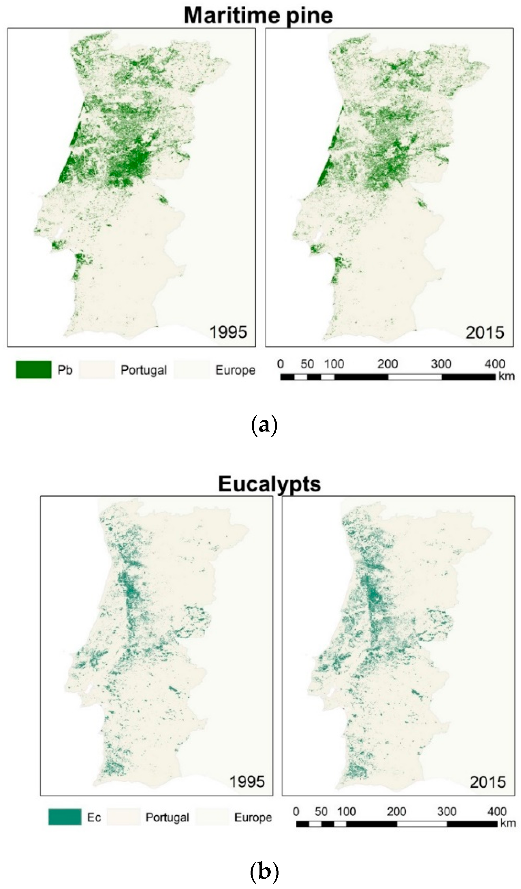
2.1.2. Species Forests Cover (1995 and 2015)

To obtain maritime pine and eucalypts forests cover, the national reference thematic map for Land Cover and Land Use (LCLU) in Portugal named as COS (Carta de Ocupação do Solo) for 1995 (COS1995) and 2015 (COS2015) were used [35]. The COS maps have a scale of 1:25,000, one ha of the minimum cartographic unit, a five-level hierarchical classification with 89 (COS1995) and 48 (COS2015) classes in the most detailed level, available through Web Feature Services (WFS) [36], allowed a detailed analysis regarding these species’ forests cover (Figure 1). To that end, the COS1995 legend was first harmonized concerning the COS2015 legend. In this analysis, only pure forests of the species were considered (i.e., forests where the dominant species represents more than 75% of the total number of trees and the ground cover is higher than 10%) as they represent more than 80% of these species’ types of occupation [36,37].

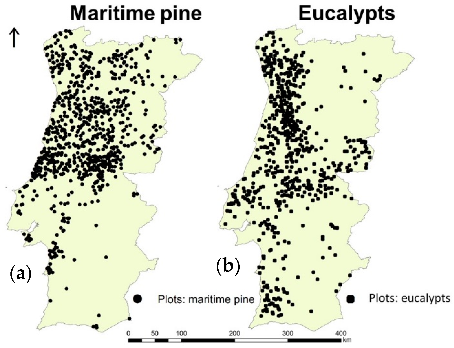
2.1.3. Species Forest Inventory (1990–1994)

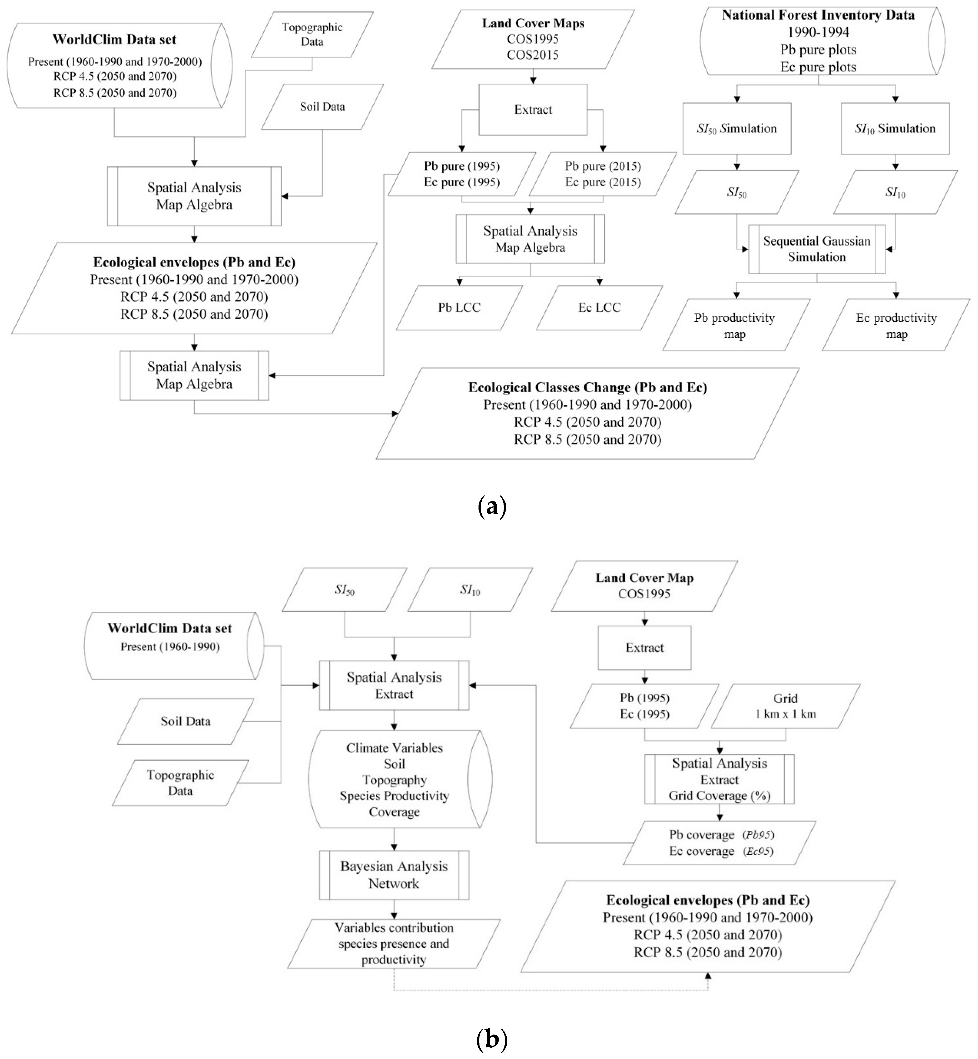
The National Forest Inventory data in 1990–1994 (NFI4) regarding the plots measured in pure stands (i.e., forests where the dominant species represents more than 75% of the total number of trees and the ground cover is higher than 10% [36,37]) of maritime pine and eucalypts were used to estimate these species productivities (Figure 2). The two-species stands characterization based on the NFI4 plots collected data [38] are synthesized in

Table 2. Summary statistics—Stands characteristics for the NFI4 plots (1990–1994).

Variable	Units	Min.	Max.	Mean	Std. dev.	Min	Max.	Mean	Std. dev.
		NFI4 plots in pure maritime pine stands (n = 744)				NFI4 plots in pure eucalypts stands (n = 615)
N	trees ha−1	10	2510	399	371	10	2770	607	486
G	m2 ha−1	0.2	57.5	13.1	11.2	0.2	59.3	8.4	6.8
V	m3 ha−1	0.0	440.6	90.7	86.9	0.0	704.9	53.7	56.9
ddom	cm	7.6	61.6	28.1	10.4	7.5	92	19.8	11.6
hdom	m	3.2	31.0	15.3	5.6	6.0	43.6	17.6	6.1
t	years	6	80	41	16	2	60	10	6

Legend: N—Number of trees per ha (trees ha⁻¹); G—Basal area per ha (m² ha⁻¹); V—Volume per ha (m³ ha⁻¹); ddom—Dominant diameter (cm); hdom—Dominant height (m); t—Age (y); n—Sample size; Min.—Minimum; Max.—Maximum; Std. dev.—Standard deviation.

.

In Portugal, maritime pine stands are mainly established by natural regeneration and managed in medium to long revolutions (e.g., more than 35 years) [11,37,39]. Eucalypts stands are installed by plantation and commonly managed throughout three rotations of short harvesting cycles (e.g., 10–12-year coppices) [8,40].

2.2. Methods

2.2.1. Species Ecological Envelopes Maps

The distribution of maritime pine in Portugal (Figure 1a) corresponds to a coastal strip that extends from the Sado and the Tejo rivers basins to the Minho river basin, penetrating in the north and center inland up to elevations of 700–900 m, preferably in the southwest to north-facing slopes where the Atlantic influence is still felt. Its climatic optimum corresponds broadly to an average temperature between 13 and 15 °C, an average temperature of the coldest month between 8 and 10 °C, and average annual precipitation between 500 mm and 1200–1400 mm. Regarding elevation, basal regions (0–400 m) are the most favorable. The species has severe limitations to growth above 800 m, due to wind and snow and has increased susceptibility to pests and diseases [40]. The species does not support well intense and prolonged colds and snow. As a pioneer species, it grows well in poor soil with light textures, preferably siliceous [39].

Eucalypts’ present-day distribution in Portugal (Figure 1b) includes areas of precipitation between the 700–2000 mm and mild winter due to its sensitivity to frost, in the north-coastal and central-coastal regions (Figure 1b) [38]. The species thrives in soil with a certain amount of humidity, well-drained, and without active limestone [7]. Data on eucalypts species naturalization in Portugal, showed that E. globulus is able to naturally regenerate from seeds both inside and outside plantations, corroborating that precipitation and distance to the sea (used as a surrogate of thermal amplitude) are key factors for the abundance of this species wildlings [9]. But topography, frost occurrence, and soil type also play a significant role [9]. Indeed, Catry et al. [9] observed that wildlings abundance, measured as the plant density through the number of plants per hectare, peaked at around 1500 mm of annual precipitation and it decreased with both low and high precipitation, reaching the lowest values below 800 mm and above 2400 mm. Higher plant density was also found in areas with milder temperatures, namely closer to the sea (with lower thermal amplitude) and with a lower number of days with frost. Plant density also seemed to be favoured in areas with intermediate elevation, higher slope and with certain soil types (namely, Cambisols and Podzols) [9]. These results are consistent to the previous knowledge for the species [38] and allow to understand what climate and site conditions this species natural regeneration prefers. Thus, helping to define the environmental variables range for the species site suitability. It should be noted that wildlings abundance is not a site productivity indicator and will be treated further in Section 2.2.3.

The species ecological envelopes for maritime pine and eucalypts [26], based on the species distribution information obtained in the literature [27], are defined by the following five variables: (i) temperature range (T max Aug–T min Jan); (ii) temperature limits (T max Aug and/or T min Jan); (iii) precipitation (P, i.e., BIO12); (iv) elevation (E); and (v) lithology. The variable thresholds (

Table 3. Variables and thresholds defining species ecological envelopes [25].

	Temperature Range (°C)	Temperature Limits (°C)	Precipitation (mm)	Elevation (m)	Lithology
Maritime pine	T max Aug–T min Jan < 26	T max Aug < 29.9	P > 850	E < 800	different of Limestone
Eucalypts	T max Aug–T min Jan < 26	T max Aug <31 T min Jan > 2	P > 600	E < 500	different of Limestone and Wind alluvial sands

Legend: T max Aug—Maximum temperature in August (˚C); T min Jan—Minimum temperature in January (˚C); P—Annual precipitation (mm; BIO12); E—elevation (m).

) ensure that more than 75% of the species forest inventory plots (IFN4), as a dominant species, are inside of the envelope. The maps of the input variables are reclassified by the Boolean method (0—Not suitable, 1—Suitable). The species ecological envelopes maps are obtained by map algebra, by summing the species variable maps produced earlier, resulting in five suitability classes classification as follows: (5) Excellent, (4) Good, (3) Regular, (2) Marginal, and (1) Unsuitable [25].

In this study, the above-referenced methodology was used to produce the species ecological envelopes by using both the present climate data for 1960–1990 (Table 3 and Figure 3) and 1970–2000. The resulting envelopes were then applied using the predicted future climate data for 2050 and 2070 under the two RCPs scenarios (RCP 4.5—Meeting the Kyoto goal; and RCP 8.5—Not meeting the Kyoto goal). Afterwards, the ecological envelope classes area for both species in Portugal was extracted to analyze the country species potentiality in the present (1960–1990 and 1970–2000) and in future scenarios (2050 and 2070, both under RCP4.5 and RCP 8.5 scenarios).

2.2.2. Species Forests Cover Distributions (1995 and 2015)

The main change trends regarding these two-species are well known. From 1995 to 2010, the maritime pine forest area decreased by 27% while eucalypts forest areas observed an increase of 13%, mainly by the reconversion of maritime pine areas after fire [11]. In this study, the land cover change map for the 20-year period (1995–2015) was performed, with a 1 km spatial resolution, by map algebra (subtraction) of the species forest cover in 1995 and 2015 (from COS1995 and COS2015).

The area of the ecological envelope classes over both species distributions in 1995 (COS1995) was extracted to analyze the potentiality of species forest areas (present and 2050 and 2070, both under RCP4.5 and RCP 8.5 scenarios). The ecological envelope classes change over both species distributions in 1995 (COS1995) was also performed by map algebra (subtraction) of the present and future scenarios (2050 and 2070, both under RCP4.5 and RCP 8.5 scenarios) to analyze the change trends in both species’ potential areas.

The same grid (1 km × 1 km) was used to extract for each pixel the two-species percentage coverage in the COS1995 (Figure 1; Pb95 and Ec95; species presence occurs when pixel percentage coverage is higher than 0) and the correspondent bioclimatic (1960–1990), topographic and soil variables (Table 1). The species presence was searched in every COS class where the species is mentioned. These data (

Table A1. Summary statistics: Species presence in COS 1995 (maritime pine—Pb95; and eucalypts—Ec95); species productivity in 1990–1994 plots (maritime pine—SI₅₀; and eucalypts—SI₁₀) and the correspondent climatic (1960–1990), topographic and soil variables.

Variable	Units	Min.	Max.	Mean	Std. Dev.	Min.	Max.	Mean	Std. Dev.	Min.	Max.	Mean	Std. Dev.
		Presence—Pb95 and Ec95 (n = 88,496)				Maritime pine—SI50 (n = 740)				Eucalypts—SI10 (n = 614)
Pb95	%	0.0	100.0	6.6	16.5
Ec95	%	0.0	100.0	9.6	20.0
SI50	m					5.8	48.6	18.4	4.4
SI10	m									4.7	37.4	19.1	4.0
T max	°C	9.9	22.8	19.7	1.9	4.5	13.1	9.9	1.5	16.1	22.2	19.7	1.2
T min	°C	2.7	13.2	10.2	1.9	13.0	21.9	19.0	1.4	7.4	12.8	10.5	1.2
BIO1	°C	6.3	17.6	15.0	1.8	9.5	17.5	14.5	1.4	11.8	17.1	15.1	1.1
BIO2	°C	5.2	11.7	9.5	1.0	5.8	11.0	9.1	0.9	6.0	11.2	9.1	0.9
BIO3	%	31.0	51.0	40.0	2.4	31.0	46.0	40.4	2.7	35.0	45.0	41.1	2.2
BIO4	%	26.0	61.2	48.6	7.2	29.8	60.6	44.7	0.7	29.5	60.5	46.2	0.7
BIO5	°C	19.7	34.0	28.6	2.5	22.1	31.9	27.3	2.1	22.4	32.7	27.6	2.4
T max Aug	°C	19.7	33.7	28.6	2.5	20.9	28.9	24.8	1.4	20.8	29.9	25.5	1.7
BIO6	°C	−2.8	9.2	5.0	2.3	−1.1	8.3	4.8	1.9	1.4	8.4	5.6	1.5
T min Jan	°C	−4.6	10.0	2.8	2.0	−2.6	8.4	3.0	2.0	0.3	7.7	3.6	1.4
BIO7	°C	12.2	29.3	23.6	2.9	14.1	27.9	22.5	2.9	14.4	27.8	22.0	2.7
BIO8	°C	0.5	13.7	9.5	2.5	3.4	13.1	9.1	2.1	5.4	13.1	10.1	1.5
BIO9	°C	13.6	24.9	21.2	1.7	16.8	23.8	20.4	1.3	17.4	24.4	20.8	1.5
BIO10	°C	13.6	25.0	21.4	1.8	16.8	23.8	20.6	1.4	17.6	24.5	21.0	1.6
BIO11	°C	0.5	13.0	9.0	2.3	2.8	12.3	8.8	1.9	5.4	12.2	9.6	1.4
BIO12	mm	463.0	1792.0	840.7	269.9	483.0	1593.0	1015.2	211.7	503.0	1542.0	937.1	246.8
BIO13	mm	64.0	272.0	121.5	38.5	76.0	248.0	146.7	30.0	75.0	240.0	134.0	32.4
BIO14	mm	0.0	37.0	8.0	5.8	1.0	30.0	10.6	4.4	1.0	28.0	9.2	5.1
BIO15	%	39.0	72.0	56.4	5.4	43.0	71.0	54.8	3.5	48.0	70.0	55.7	4.5
BIO16	mm	180.0	719.0	345.4	102.6	220.0	657.0	413.0	79.9	220.0	619.0	383.5	91.4
BIO17	mm	13.0	157.0	51.7	25.5	14.0	132.0	65.2	19.5	16.0	123.0	58.1	23.0
BIO18	mm	15.0	161.0	54.8	27.6	17.0	143.0	70.2	22.6	18.0	137.0	64.1	27.8
BIO19	mm	168.0	719.0	341.0	104.3	202.0	657.0	409.5	81.3	207.0	619.0	378.3	91.9
E	m	0.0	1921.0	321.0	262.6	0.0	1275.0	329.1	248.7	8.0	752.0	231.2	155.3
S	%	0.0	25.4	2.8	3.0	0.1	20.2	3.6	3.4	0.0	17.4	2.9	2.5
A	°	0.0	360.0	188.7	103.4	0.0	360.0	197.7	97.9	0.0	359.7	198.4	99.7
WRBFU		2.0	130.0	86.2	33.8	27.0	124.0	83.8	38.1	27.0	127.0	85.3	36.1

Legend: Pb95—Maritime pine presence in 1995 (pixel percentage coverage); Ec95—Eucalypts presence in 1995 (pixel percentage coverage); SI₅₀—hdom (m) at the age of 50 years; SI₁₀—hdom (m) at the age of 10 years; T max—monthly average maximum temperature (°C); T min—monthly average minimum temperature (°C); BIO1—Annual mean temperature (°C); BIO2—Mean diurnal range (°C); BIO3—Isothermality (%); BIO4—Temperature seasonality (%); BIO5—Maximum temperature of the warmest month (°C); T max Aug—Maximum temperature in August (°C); BIO6—Minimum temperature of the coldest month (°C); T min Jan—Minimum temperature in January; BIO7—Temperature annual range (°C); BIO8—Mean temperature of the wettest quarter (°C); BIO9—Mean temperature of the driest quarter (°C); BIO10—Mean temperature of the warmest quarter (°C); BIO11—Mean temperature of the coldest quarter (°C); BIO12—Annual precipitation (mm); BIO13—Precipitation of the wettest month (mm); BIO14—Precipitation of the driest month (mm); BIO15—Precipitation seasonality (%); BIO16—Precipitation of the wettest quarter (mm); BIO17—Precipitation of the driest quarter (mm); BIO18—Precipitation of the warmest quarter (mm); BIO19—Precipitation of the coldest quarter (mm); E—Elevation (m); S—Slope (%); A—Aspect (°); WRBFU—soil codes; n—sample size; Min.—minimum; Max.—maximum; Std. dev.—standard deviation.

in Appendix A) were used in a machine learning approach to gauge variable influence in these two-species distributions (Figure 4).

2.2.3. Species Productivity Maps

In Portugal, the annual average maritime pine productivity (for fully mature trees of 35–45 years old) is about 5–10 m³ha⁻¹y⁻¹ of timber in the north of the Tagus river, and lowers, in general, to 4 m³ha⁻¹y⁻¹ in the south of the Tagus river. Much lower productivities of 0.7–3.4 m³ha⁻¹y⁻¹, are found in poor-quality areas, such as plots in coastal dunes [41]. In the coastal center regions maritime pine achieves the highest productivities (e.g., mean annual increment higher than 13.3 m³ha⁻¹y⁻¹, at the age of 30 years old), followed by the northern and central montane and submontane regions (e.g., around 10.3 m³ha⁻¹y⁻¹) [42].

Eucalypts have higher productivities in the Atlantic seaboard (e.g., higher than 15 m³ha⁻¹y⁻¹) followed by the Tagus valley region (e.g., between 10 and 15 m³ha⁻¹y⁻¹; mean annual increment at the age of nine years old of eucalypts plantations without genetic improvement). In low productivity regions for this species, such as the inland of the country, productivities can be lower than 10 m³ha⁻¹y⁻¹ [43].

To assess the two-species productivities, the most widely accepted site productivity indicator, the site index, as used [44]. As forest site productivity is very dependent on both environmental and biotic factors present at the site where the forest species is present [44], the most recent prediction models including environmental parameters, for each species site index evaluation, were selected [45,46,47].

The site index assessment for the NFI4 maritime pine plots was performed using the empirical model developed by Nunes et al. [45], a multiple asymptotes polymorphic equation from Cieszewski [48], modified to include parameters related to climate and soil characteristics (P or BIO12, T or BIO1, WINTER or BIO6, and ST₁, ST₂, ST₃;

Table 4. Site index models for the species maritime pine [45] and eucalypts [46,47].

Species	Site Index Model
Maritime pine SI50—Dominant height at the reference age of 50 years	$S{I}_{50}=e^X{e}^{\left(-\left(b_1+\frac{1}{X}\right){50}^{-c}\right)}$ $X=0.5\left(b_1{t}^{-c}+\ln \left(hdom\right)+F\right)$ $F={\left({\left(b_1{t}^{-c}+\ln \left(hdom\right)\right)}^2+4t^{-c}\right)}^{0.5}$ with, $b_1=9.2562-0.0006\frac{P\sqrt{T}}{WINTER}$ $c=0.5394-0.0918 S{T}_1-0.1767\left(S{T}_2+S{T}_3\right)$ where hdom—Dominant height (m); t—Stand age (y); P—Annual precipitation (mm; BIO12); T—Annual mean temperature (°C; BIO1); WINTER—Type of winter in a scale from 1 to 5 (1—warm (<7 °C); 2—temperate (3–7 °C); 3—fresh (0–3 °C); 4—cold (−3–0 °C); 5—very cold (<−3 °C; BIO6); ST1, ST2, ST3—Dummy variables for humic cambisols, rankers and calcic cambisols, respectively.
Eucalypts SI10—Dominant height at the reference age of 10 years	$S{I}_{10}=\left(29.0669+0.2880.dp\right){\left(\frac{hdom}{29.0669+0.2880.pd}\right)}^{{\left(\frac{t}{10}\right)}^{0.4890}}$ where pd—number of precipitation days per year with values greater than 0.1 mm; hdom—dominant height (m); t—stand age (y).

and

Table 5. Reference productivity classes [42,44,45,46].

Class	Productivity	Maritime Pine SI50 (m)	Eucalypts SI10 (m)
1	High	≥24	≥23
2	Medium-High	20–24	20–23
3	Medium	16–20	17–20
4	Low-Medium	12–16	14–17
5	Low	<12	<14

Legend: SI₅₀—hdom (m) at the age of 50 years; SI₁₀—hdom (m) at the age of 10 years.

). The parameters were obtained from the climate data set from the WorldClim (1960–1990), the elevation data from STRM (Shuttle Radar Topography Mission), and the soil data from the ESDBv2 Raster Library (Table 1).

The site index assessment for the NFI4 eucalypts plots was performed using the empirical model developed by Tomé et al. [46,47] that includes one parameter related to climate (pd—Number of precipitation days per year; Table 4 and Table 5). Regarding the climate parameter pd (Table 4) the observations from Portuguese meteorological stations in three temporal 30-year series (1931–1960, 1951–1980 and 1971–2000) were used [49,50,51,52,53,54]. After, the pd climatic parameter was interpolated using the Inverse Distance Weighted (IDW) algorithm. The allocated weight was the local correspondent elevation (E) of the species NFI4 plots.

Afterwards, to obtain the species productivities maps (Maritime pine site index—SI₅₀; and Eucalypts site index—SI₁₀), the data spatial characterization was performed through a 2-step approach.

Firstly, the structural analysis through variography, omnidirectional experimental variograms were computed and the best fitted theoretical models adjusted [55]. For computation, SpaceStat V. 4.0e0.18. software [56] was used.

The variogram is a vector function used to compute the spatial variability of regionalized variables defined by the following equation:

$$\gamma \left(h\right)=\frac{1}{2N\left(h\right)}{\displaystyle \sum }_{2N\left(h\right)}^{N\left(h\right)}{\left[Z(x_i-Z\left(x_i+h\right)\right]}^2$$

(1)

Its argument is h (distance) where Z (x_i) and Z (x_i + h) are the numerical values of the observed variable at points x_i, and x_i + h. The number of forming pairs for h distance is N (h). Thus, it is the average value of the square of the differences between all pairs of points in the geometric field spaced at h distance. The graphic study of the variograms obtained provides an overview of the spatial structure of the variable. The nugget effect (C₀) shows the behavior at the origin, whereas the sill (C₁) and the amplitude (a) define the variance used in the subsequent interpolation steps and the spatial influence of the variable, respectively.

Secondly, a Sequential Gaussian Simulation (SGS) was used as a stochastic approach used to map the two-species productivities’ spatial distribution, through the construction of 100 scenarios. SGS starts by defining the univariate distribution of values followed by a normal score transform of the original values to a standard Gaussian distribution. Simulation of the obtained normal scores at grid node locations is done sequentially with simple kriging (SK) using the normal score data and a zero mean [57]. Once all normal scores have been simulated, they are back-transformed to original grade values. The result of a simulation process is a twisted version of an estimation process, which reproduces the statistics of the known data, making a realistic view, but supplying a low prediction behavior. Nevertheless, if multiple sequences of simulations are designed, it is possible to obtain more reliable probabilistic maps. The average image was computed, together with the associated standard deviation for the spatial uncertainty visualization [58].

Finally, the resulting productivity mean images (MI) and the spatial uncertainty representation, through standard deviation (SU), with a 2.45 km × 2.45 km resolution, were reclassified in five productivity classes using the statistical criteria of Jenks natural breaks [59].

Afterwards, for each maritime pine and eucalypts NFI4 plots (1990–1994), the simulated site indices (SI₅₀ and SI₁₀, respectively) and the correspondent climatic (1960–1990), topographic and soil variables were extracted (Table 1). These data (Table A1) were used in a machine learning approach to gauge variable influence in these two-species productivities (Figure 4).

2.2.4. Variables Influence Analysis in Species Distribution and Productivity

Bayesian networks have become extremely popular for gaining deep insight into manifold problem domains [60]. Their inherently graphical structure built upon machine learning algorithms based on the Bayesian Network formalism leads to robust models optimal for exploring and explaining complex problems. In this study, four supervised Bayesian networks machine-learned from the data (i.e., presence—Pb95 and Ec95 and productivity—SI₅₀ and SI₁₀) were created to assess the most influential variables conditioning maritime pine and eucalypts distribution and productivity. To measure the variable influence regarding the target node (X) of each network, first, the relative mutual information (RMI) was calculated to quantify the percentage of information gained on X by observing Y

$$RMI\left(X,Y\right)=\frac{MI\left(X,Y\right)}{H\left(X\right)}$$

(2)

where $MI\left(X,Y\right)$ is the mutual information [61] in absolute terms and $H\left(X\right)$ the entropy associated with the probability distribution of X. The entropy of a variable can also be understood as the sum of the expected log-losses of its states. Both metrics are expressed in bits and can be calculated as follows

$$MI\left(X,Y\right)=H\left(X\right)-H\left(X|Y\right)$$

(3)

$$H\left(X\right)=-{\displaystyle \sum }_{xϵX}p\left(x\right){\log }_2\left(p\left(x\right)\right)$$

(4)

where H (X|Y) is the conditioned entropy associated with the probability of X given Y (how likely is X if you learn Y) and p(x) is the probability of x.

From the RMI analysis, a ranking was obtained regarding the significance of each variable to the knowledge of the target node. However, due to the high dispersion, the large number of variables might be introduced in the model, a second measurement was conducted with the most influential variables identified by the RMI analysis. The Bayesian models were machine-learned again in a simplified scheme and a contribution analysis was computed, showing the contribution of each variable towards the predicted mean of the target variable (i.e., presence—Pb95 and Ec95 and productivity—SI₅₀ and SI₁₀). The contribution of each variable is estimated using counterfactuals based on a specific neutral state that represents the neutral condition of the system. For modeling and graphical representation, the Artificial Intelligence software BayesiaLab 9 [62] was used.

The Bayesian machine learning analysis for the data (i.e., presence—Pb95 and Ec95 and productivity—SI₅₀ and SI₁₀) was carried out with the Augmented Naïve Bayes algorithm. The architecture of this algorithm is rooted in a naive architecture (the target node is the parent of all the other nodes), enhanced by the relations of the child nodes [63]. Cross-validation was used to estimate the prediction accuracy of the supervised machine learning models created. The relative significance (RS), as the ratio between the mutual information brought by each variable and the maximum mutual information, which corresponds with the most informative variable, was used to interpret these results. Due to the informative dispersion by the large number of variables introduced in the model, a closer look into the variables with the highest RS was done, which were taken to a second step to build a simplified Bayesian network (RS > 70% and RMI sum > 80%)

In the end, the open-source software WEKA [64] was used to fit Machine Learning (ML) regression tree models by the algorithm Random Forest [65,66] to compare the quality of ecological envelopes variables as regressors to the ones selected by the Bayesian network analysis.

3. Results

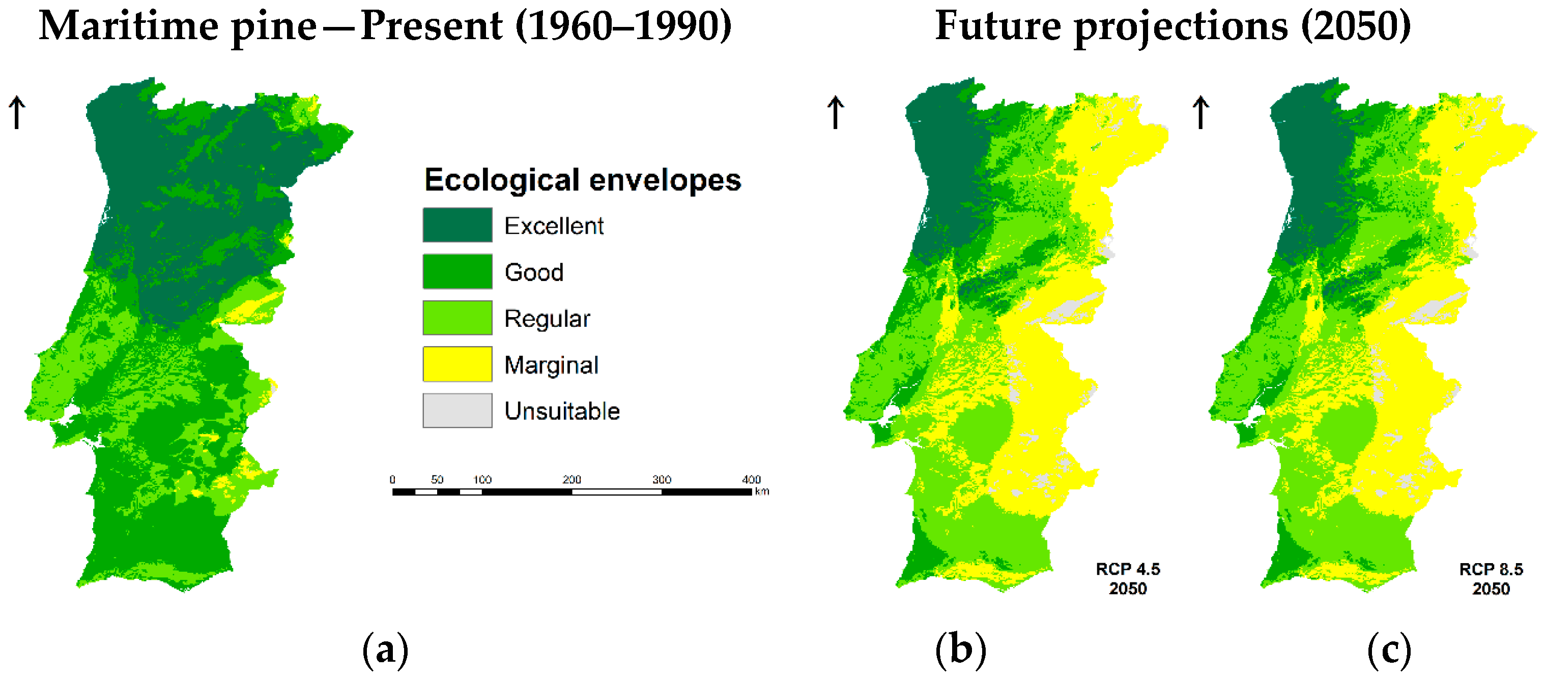
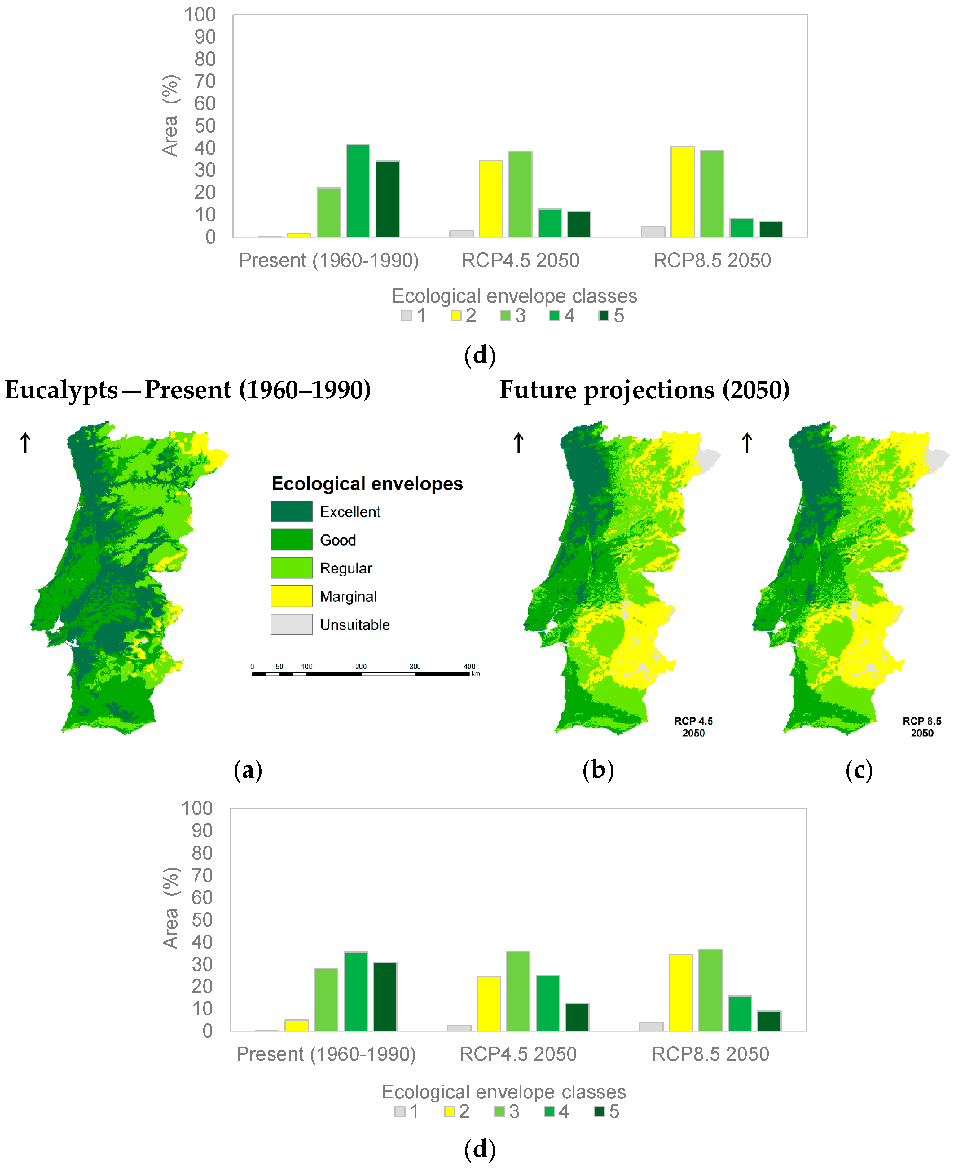
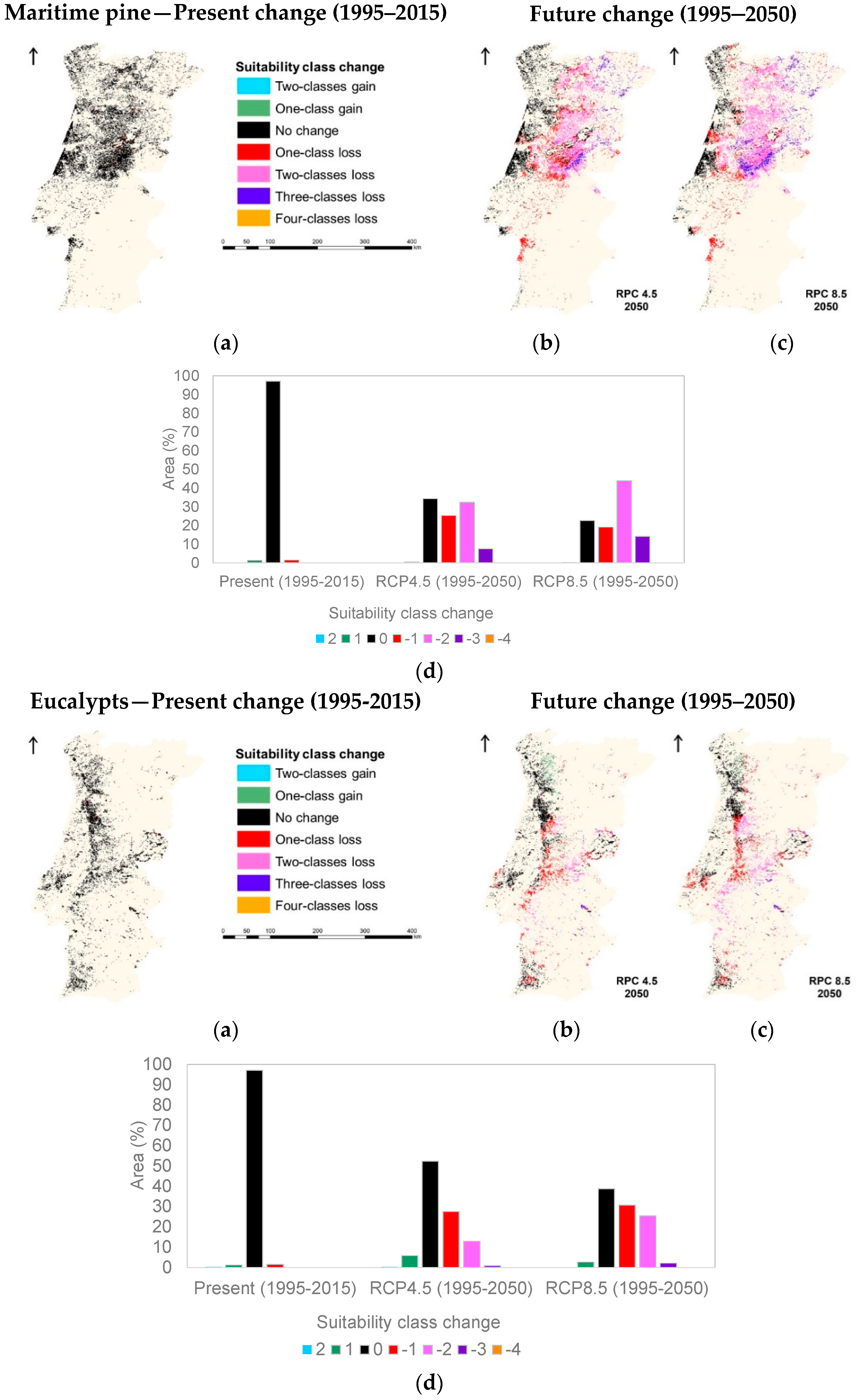
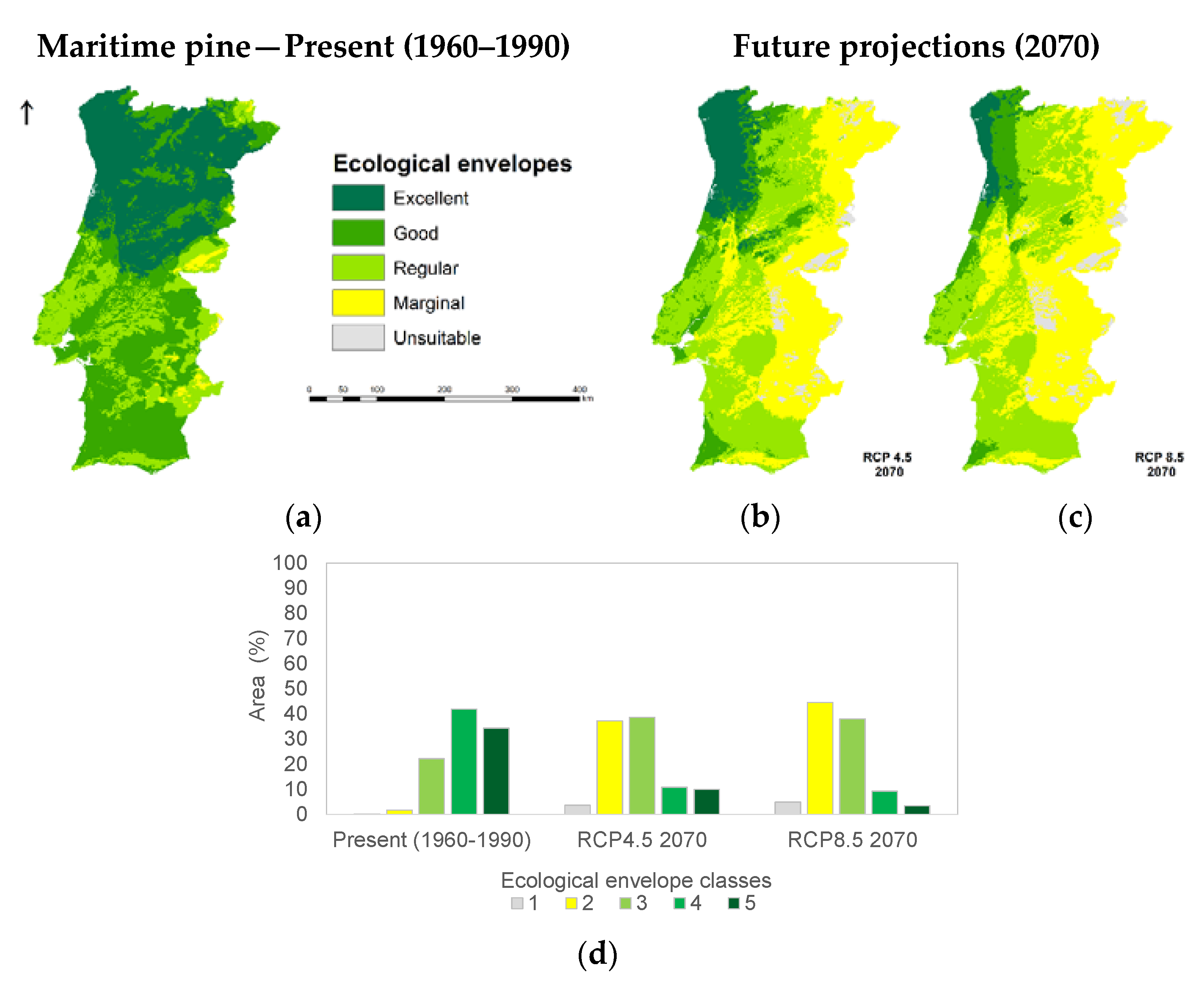
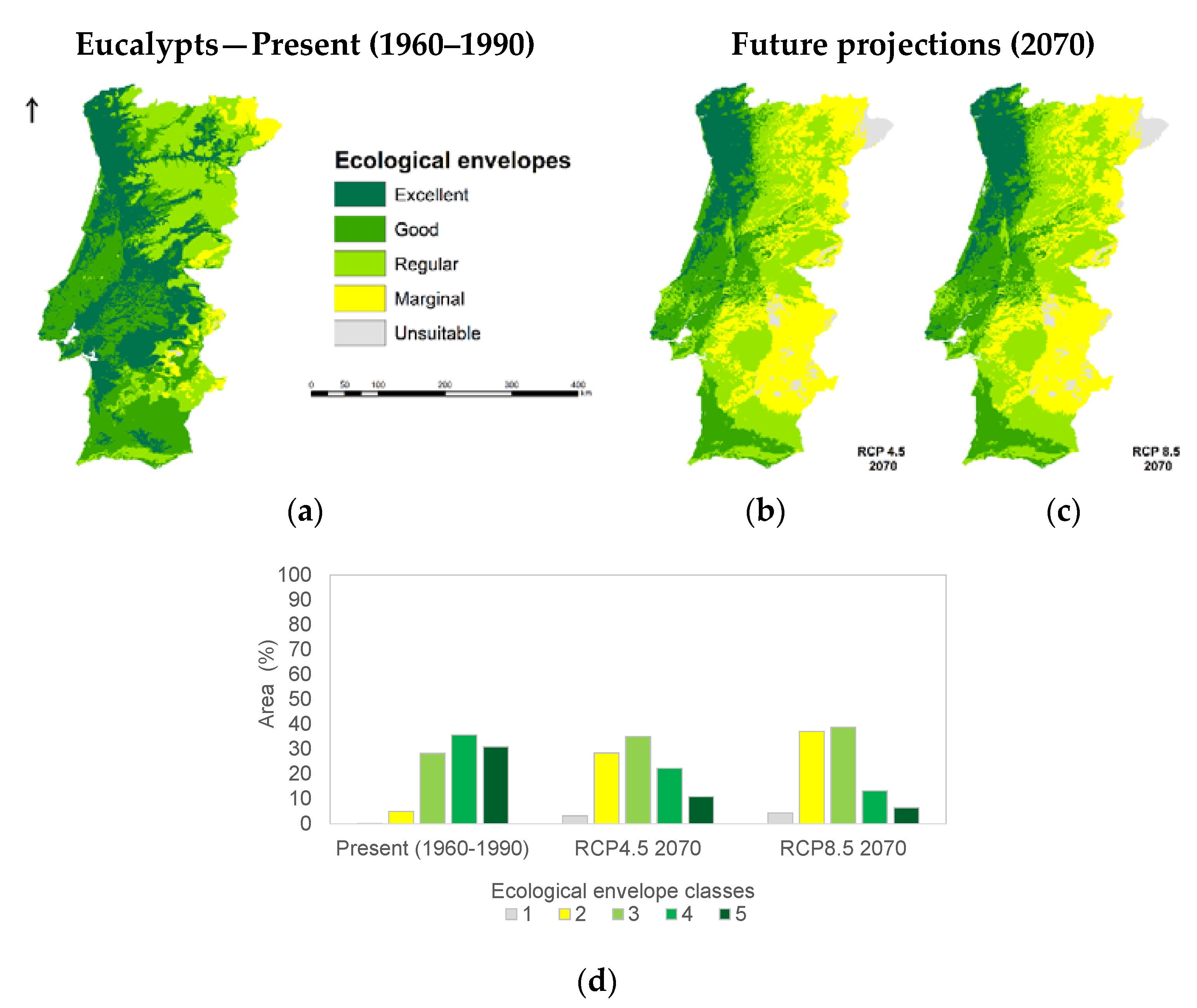
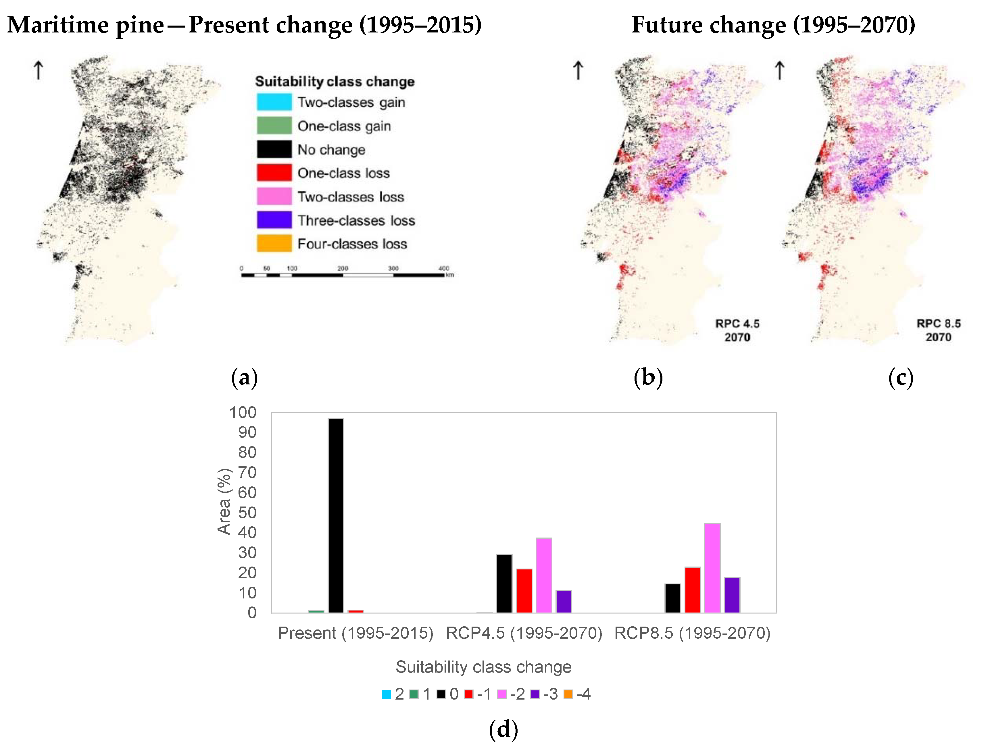
3.1. Species Ecological Envelopes under the Climate Scenarios

The ecological envelope maps analysis for both species in Portugal (Figure 5a,d) indicates that, in the present (1960–1990), the country’s area potentiality for maritime pine is distributed as follows: 34% excellent, 42% good, and 22% regular. For eucalypts, the country’s area potentiality is distributed where 31% is excellent, 36% is good, and 28% is regular. Therefore, in Portugal, there is a high potential for both species’ afforestation (an area over 95%).

Likewise, when analyzing the ecological envelope maps in the present, but now with the climate data sets from 1970 to 2000, little change was observed and the high potentiality for both species’ afforestation maintains.

Ecological envelope maps projected for future scenarios in 2050 (Figure 5b—RCP4.5; Figure 5c—RCP8.5; Figure 5d), showed a decrease in the country’s area potentiality (excellent, good, and regular areas) for both species. Maritime pine potential area is expected to decrease to 63–54%, respectively, in the RCP4.5 scenario and the RCP8.5 scenario. However, for eucalypts the decrease will not be so severe, ranging to 73–62%, respectively, in each scenario.

The ecological envelope maps for the projected future scenarios in 2070 are very similar to the ones in 2050. However, the maritime pine potential area is expected to decrease further to 59–51%, respectively, in the RCP4.5 scenario and RCP8.5. Similarly, for eucalypts, the decrease is expected to be 68–59%, respectively, in each scenario (Figure A1).

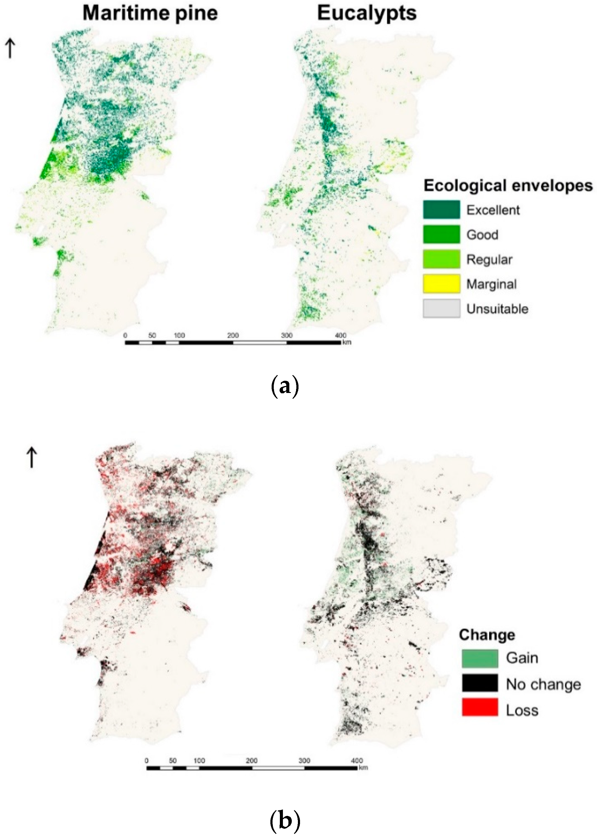
3.2. Species Forests Cover Distributions Maps

Comparing the ecological envelope classes (Figure 5a) over the present species distributions in 1995 (COS1995; Figure 1) it was verified that 99% of maritime pine forest and eucalypts forest were found inside excellent, good and regular ecological envelope classes (Figure 6a). In fact, 62% of the maritime pine forest is inside the excellent class (Figure 6a) compared to 52% of the eucalypts forest (Figure 6a).

Moreover, according to the known land cover trend between these two species, the maritime pine forest has experienced a reduction between 1995 and 2015 which was mostly replaced by eucalypts new afforestation (Figure 6b).

Little change was observed for the ecological envelope maps in the present, obtained using the climate data sets from 1970 to 2000 instead (Figure 7a).

In 2050 future scenarios (Figure 5b,c), the maritime pine forest area (Figure 1a) will lose potentiality by decreasing from 99% to 84–72%, respectively, in each scenario (Figure 7b–d). Nevertheless, for the eucalypts forest area (Figure 1b) the potentiality loss will be lesser than for maritime pine, decreasing only to 91–85%, respectively, in each scenario (Figure 7b–d). Indeed, maritime pine forest in excellent areas class will experience a great loss in potentiality, from 62% to 19–11%, respectively, in each scenario (Figure 5b–d). Conversely, the eucalypts forest showed a much lesser decrease, from 52% to 32–22%, respectively, in each scenario (Figure 5b–d). The loss of maritime pine forest area potential is more severe in the north inland of the country (three-class dropdown) followed by the central north (two-class drop drown; Figure 7b–d). However, the loss of the eucalypts’ forest area potential will occur in the inland (three-class drop drown) followed by the center (two-class dropdown; Figure 7b–d).

Once more, the projected future scenarios in 2070 are very similar to the ones in 2050. However, the maritime pine forest area (Figure 1a) will continue to lose potentiality by decreasing to 78–65%, respectively, in each scenario (Figure A2). Again, the eucalypts forest area (Figure 1b) potentiality loss will be lesser than for maritime pine, decreasing only to 89–82%, respectively, in each scenario (Figure A2). Maritime pine forest in excellent areas class is expected to lose potentiality to 15–6%, respectively, in each scenario (Figure A1). Eucalypts forest will continue showing a much lesser decrease to 28–13%, respectively, in each scenario (Figure A1).

The same analysis was performed regarding the species distributions in 2015 (COS 2015; Figure 1) but only a small percentage variation (ranging ±3%) was observed.

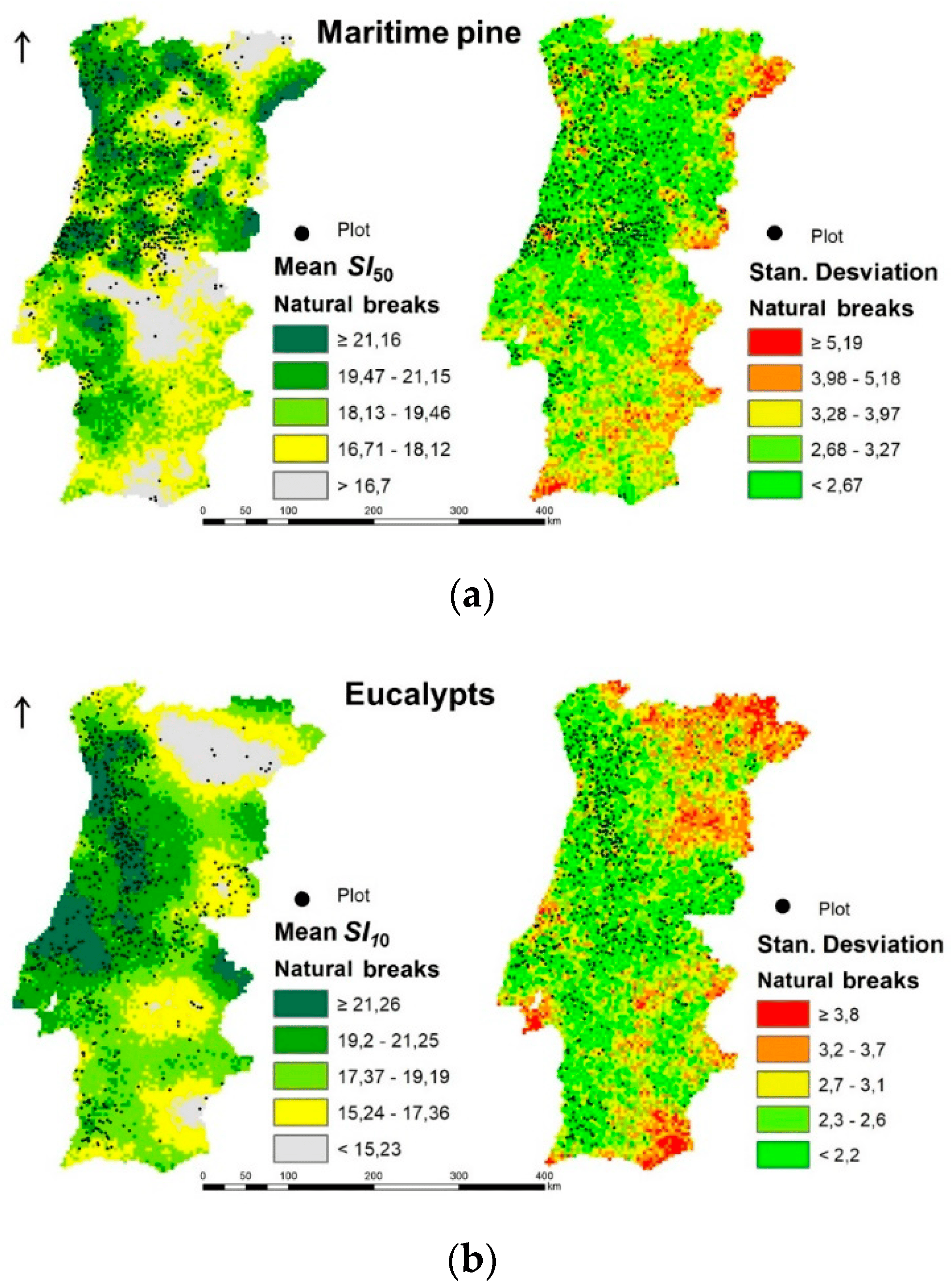
3.3. Current Climate Species Productivities Maps

The two-species current productivities maps (Figure 8), obtained from the National Forest Inventory data in 1990–1994 (NFI4), show high productivity areas for maritime pine (SI₅₀ > 21.15 m) mainly in the west-northern and the center of the country (Figure 8a), and for eucalypts (SI₁₀ > 21.27 m) mainly in a western strip in the center and north of the country (Figure 8b). Inland regions are associated with high spatial uncertainty, while coast regions are associated with low spatial uncertainty, as expected due to those species’ present distributions (Figure 1). The productivity classes, obtained by using the statistical criteria of Jenks natural breaks, are less restrictive than the ones found in the literature (Table 5). The species highest productivities were found overlapping areas from regular to excellent ecological envelope classes, namely, 68% for maritime pine and 56% for eucalypts (Figure 6 and Figure 8).

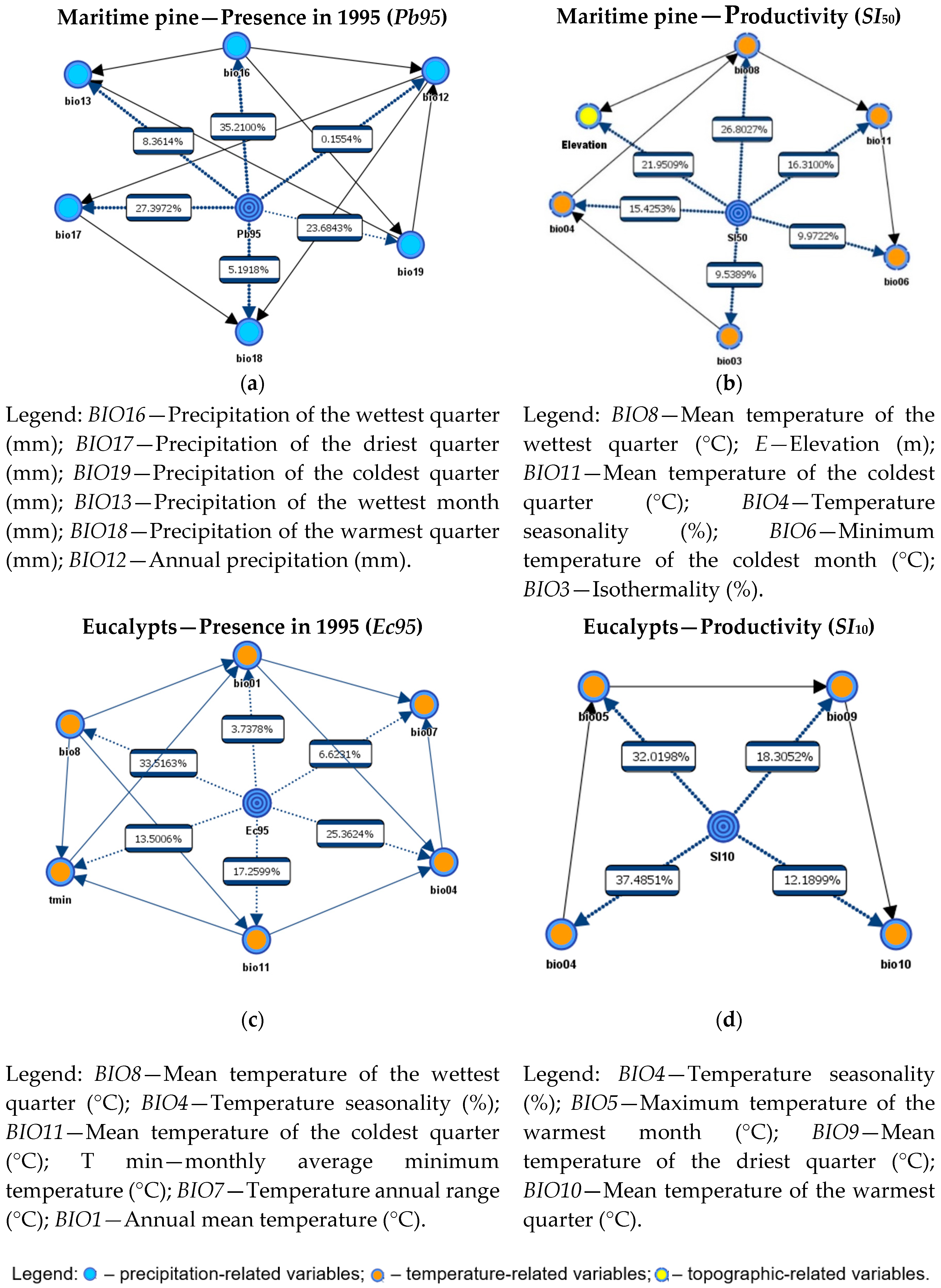
3.4. Variables Influence Analysis in Current Species Distribution and Productivity

The Bayesian machine learning analysis was performed for the two-species current distributions (Pb95 and Ec95) and productivities (SI₅₀ and SI₁₀). The cross-validation indicated that Bayesian models for species presence showed a higher quality of the problem representation than those for productivity. The contingency table fit (CTF) values for Pb95 and Ec95 (above 85%) indicate that the joint probability distribution by the created networks is good. In turn, the CTF values for SI₅₀ and SI₁₀ are slightly lower, ranging from 70% to 80%. This circumstance can be appreciated when comparing the RMI for the species presence and productivity (

Table A2. Bayesian networks—Relative Mutual Information (RMI) and Relative Significance (RS): species presence (maritime pine—Pb95; and eucalypts—Ec95); species productivity (maritime pine—SI₅₀; and eucalypts—SI₁₀) and the correspondent climatic (1960-1990), topographic and soil variables (most contributive variables highlighted in bold—RS > 70% and RMI sum > 80%).

Variable	Pb95		Ec95		SI50		SI10
	RMI (%)	RS (%)	RMI (%)	RS (%)	RMI (%)	RS (%)	RMI (%)	RS (%)
T max	5.95	57.61	3.91	62.16	0.95	44.09	2.14	60.02
T min	6.60	63.83	5.54	88.01	1.43	66.24	1.54	43.26
BIO1	6.02	58.24	4.60	73.06	1.44	66.36	2.12	59.30
BIO2	3.75	36.27	3.73	59.31	0.81	37.15	0.85	23.94
BIO3	1.94	19.18	3.86	61.38	1.63	75.38	1.67	46.75
BIO4	2.97	28.74	5.32	84.45	1.62	74.88	3.07	85.79
BIO5	3.42	33.15	2.60	41.35	1.09	50.38	3.58	100.00
BIO6	2.54	24.58	0.53	8.41	1.77	81.97	0.63	17.61
BIO7	3.19	30.88	5.38	85.45	1.36	62.99	2.27	63.63
BIO8	5.88	59.88	6.30	100.00	2.16	100.00	0.58	16.22
BIO9	3.80	36.79	2.32	36.83	0.72	41.50	2.98	83.37
BIO10	4.41	42.66	2.28	36.25	0.71	33.16	3.02	84.50
BIO11	5.57	53.89	5.50	87.35	1.96	90.52	1.01	28.03
BIO12	10.27	99.40	2.64	41.99	0.59	27.52	1.59	44.62
BIO13	9.91	95.89	4.15	65.99	1.14	52.71	1.35	37.92
BIO14	5.91	57.22	0.97	15.46	0.33	15.45	1.26	35.36
BIO15	5.78	55.54	2.40	38.24	0.96	44.76	1.34	37.87
BIO16	10.21	98.73	3.08	48.99	0.55	25.69	1.65	46.29
BIO17	8.32	80.45	1.77	28.18	0.72	32.90	1.02	28.51
BIO18	8.80	85.12	1.19	18.95	0.81	37.45	1.09	30.70
BIO19	10.34	100.00	3.12	49.57	0.87	26.33	1.60	44.44
Elevation	1.99	19.27	2.91	46.31	1.95	90.34	0.56	15.64
Slope	0.92	8.99	0.40	6.36	1.25	58.07	0.25	7.23
Aspect	0.11	1.12	0.10	1.60	0.34	15.88	0.46	13.11
WRBFU	1.02	9.95	0.60	9.64	1.15	53.45	1.55	43.48

Legend Pb95—Maritime pine presence in 1995 (pixel percentage coverage); Ec95—Eucalypts presence in 1995 (pixel percentage coverage); SI₅₀—hdom (m) at the age of 50 years; SI₁₀—hdom (m) at the age of 10 years; T max—monthly average maximum temperature (°C); T min—monthly average minimum temperature (°C); BIO1—Annual mean temperature (°C); BIO2—Mean diurnal range (°C); BIO3—Isothermality (%); BIO4—Temperature seasonality (%); BIO5—Maximum temperature of the warmest month (°C); BIO6—Minimum temperature of the coldest month (°C); BIO7—Temperature annual range (°C); BIO8—Mean temperature of the wettest quarter (°C); BIO9—Mean temperature of the driest quarter (°C); BIO10—Mean temperature of the warmest quarter (°C); BIO11—Mean temperature of the coldest quarter (°C); BIO12—Annual precipitation (mm); BIO13—Precipitation of the wettest month (mm); BIO14—Precipitation of the driest month (mm); BIO15—Precipitation seasonality (%); BIO16—Precipitation of the wettest quarter (mm); BIO17—Precipitation of the driest quarter (mm); BIO18—Precipitation of the warmest quarter (mm); BIO19—Precipitation of the coldest quarter (mm); E—Elevation (m); S—Slope (%); A—Aspect (°); WRBFU—soil codes.

). The most contributive variables (RS > 70% and RMI sum > 80%) were represented in four simplified Bayesian networks (Figure 9).

Hence, for maritime pine presence (Pb95), it was observed that precipitation-related had greater contributions (BIO16 > BIO17 > BIO19 > BIO13 > BIO18 > BIO12; Figure 9a). However, for maritime pine productivity (SI₅₀) it was found that the elevation and temperature-related variables had greater contributions (BIO8 > E > BIO11 > BIO4 > BIO6 > BIO3; Figure 9b).

For eucalypts’ presence (Ec95), it was observed that temperature-related variables had greater contributions (BIO8 > BIO4 > BIO11 > T min > BIO7 > BIO1; Figure 9c). Likewise, for eucalypts’ productivity (SI₁₀), it was found that temperature-related variables had greater contributions (BIO4 > BIO5 > BIO9 > BIO10; Figure 9d).

Finally, the fitting efficiency (e.g., pseudo-coefficient of determination R²), of the ML regression models obtained by the Random Forest algorithm, using as regressors the ecological envelopes variables in comparison to the variables selected by the Bayesian network analysis were very similar. For maritime pine presence (Pb95) models, the fitting efficiency was 69% and 66%, respectively. For maritime pine productivity (SI₅₀) models, the fitting efficiency was 14% and 17%, respectively. For eucalypts’ presence (Ec95) models, the fitting efficiency was 72% and 63%, respectively. For eucalypts’ productivity (SI₁₀) models, the fitting efficiency was 34% in both cases. These results prove how robust the ecological envelopes variables are in defining species potential areas (

Table 6. Summary data for species distribution and productivity: (a) Maritime pine presence in COS 1995 (Pb95 > 0); (b) Maritime pine productivity in 1990–1994 plots (SI₅₀); c) Eucalypts presence in COS 1995 (Ec95 > 0); (d) Eucalypts productivity in 1990–1994 plots (SI₁₀).

Variable	Units	Min.	Max.	Mean	Std. Dev.	Min.	Max.	Mean	Std. dev.
		Maritime pine—Pb95 > 0 (n = 23,752)				Maritime pine—SI50 (n = 740)
BIO5	°C	21.8	32.7	27.5	2.2	22.1	31.9	27.3	2.1
T max Aug	°C	21.8	32.7	27.5	2.2	20.9	28.9	24.8	1.4
BIO6	°C	−1.4	9.0	5.4	1.7	−1.1	8.3	4.8	1.9
T min Jan	°C	−2.4	9.3	3.4	2.0	−2.6	8.4	3.0	2.0
BIO7	°C	13.3	28.2	22.1	2.9	14.1	27.9	22.5	2.9
T max Aug–T min Jan	°C	14.1	31.0	24.1	3.2	13.6	27.4	21.8	2.4
BIO12	mm	468.0	1587.0	968.3	221.3	483.0	1593.0	1015.2	211.7
E	m	0.0	1192.0	264.9	200.7	0.0	1275.0	329.1	248.7
WRBFU		2.0	129.0	82.8	37.2	27.0	124.0	83.8	38.1
		Eucalypts—Ec95 > 0 (n = 34,730)				Eucalypts—SI10 (n = 614)
BIO5	°C	21.6	33.9	27.9	2.4	22.4	32.7	27.6	2.4
T max Aug	°C	21.6	33.5	27.9	2.4	20.8	29.9	25.5	1.7
BIO6	°C	−1.4	9.1	5.7	1.6	1.4	8.4	5.6	1.5
T min Jan	°C	−2.4	9.4	3.5	1.6	0.3	7.7	3.6	1.4
BIO7	°C	12.9	29.1	22.3	2.8	14.4	27.8	22.0	2.7
T max Aug–Tmin Jan	°C	13.0	33.0	24.4	3.3	14.7	28.0	21.9	2.3
BIO12	mm	468.0	1594.0	900.3	248.2	503.0	1542.0	937.1	246.8
E	m	0.0	1192.0	245.4	184.7	8.0	752.0	231.2	155.3
WRBFU		2.0	129.0	82.9	36.3	27.0	127.0	85.3	36.1

Legend: Pb95—Maritime pine presence in 1995 (pixel percentage coverage); Ec95—Eucalypts presence in 1995 (pixel percentage coverage); SI₅₀—hdom (m) at the age of 50 years; SI₁₀—hdom (m) at the age of 10 years; BIO5—Maximum temperature of the warmest month (°C); BIO6—Minimum temperature of the coldest month (°C); BIO7—Temperature annual range (°C); BIO12—Annual precipitation (mm); E—Elevation (m); WRBFU—soil codes; n—sample size; Min.—minimum; Max.—maximum; Std. dev.—standard deviation.

).

Comparing the ecological envelopes variables summary data (Table 6), regarding species distribution (COS 1995) and species productivity (1990–1994 plots), with the thresholds for the two-species ecological envelopes (Table 3), consistency was observed in those values.

4. Discussion

The results obtained in this study revealed that: (1) the species ecological envelopes indicate that the country has presently a high potential for both species afforestation (over 95%); future climate scenarios forecasted for both species a loss of country’s area potentiality, intensified from best to worst scenario (RCP4.5 and RCP8.5), respectively: maritime pine (98%) decreasing to 63–59% in 2050 and to 54–51% in 2070 while eucalypts (95%) decreasing to 73–68% in 2050 and to 62–59% in 2070; (2) it was verified that 99% of maritime pine forest and eucalypts forest in 1995 were found inside excellent, good and regular ecological envelope classes, noting that 62% of maritime pine forest is inside the excellent class compared to the 52% of eucalypts forest; (3) the productivity maps showed that the highest productivity areas were found overlapping areas from regular to excellent ecological envelope classes, namely, 68% for maritime pine and 56% for eucalypts; and (4) the Bayesian network analysis highlighted the most effective variables explaining better the two-species presence in 1995 and their productivities. However, when comparing these selected variables and the ecological envelopes variables as regressors in ML regression tree models the fitting efficiency was very similar proving how robust the ecological envelopes methodology is. The variable thresholds used in species ecological envelopes mapping were consistent with the ones obtained in species distributions (COS1995) and species productivity (1990–1994 plots).

So, despite Portugal having currently a high potential for maritime pine and eucalypts afforestation (over 95%), it is expected that within the next 45–65 years, excellent areas for these species will be limited to a coastal strip in the north of the country, though wider for eucalypts. Moreover, it is expected that present excellent areas will change its potentiality, becoming in the future only good and regular areas for the species. Hence, marginal areas for the species will increase mainly in the inland of the country: maritime pine, from 0.2% to 19–25% and 31–36%, and eucalypts, from 1% to 9–11% and 14–16%, respectively in both scenarios (RCP4.5 and RCP8.5).

Additionally, it is worthwhile noting, when comparing the species present distribution in 1995 with the species ecological envelopes classes, that maritime pine forest was inside the excellent class, while eucalypts new afforestation has been made inside marginal classes for this species. This trend had already been observed in the central inland region of Portugal [67]. This study has also foreseen that this trend will be aggravated in future climate scenarios. Therefore, recommendations on species afforestation potential areas will be key to set back this trend. Additionally, it is important to study the impact of climate change in other Mediterranean species to be used alternatively in future afforestation.

Other studies have reported the decrease of maritime pine and eucalypts potential distribution areas in climate change scenarios, particularly in the south of the Tagus river and in the inland [2,3,4,18]. Overall, it suggested a future trend of species migration from south to north and from the interior to the coastal areas. The eucalypts and maritime pine forests productivity in the northern region may increase in future global change scenarios, mainly in sites closer to the sea and with good quality soils. In the central region, a decrease in those species’ productivity will be expected, while in the southern region it is where these two species are expected to be most affected and possibly becoming residual species [2,3,4,19].

The species ecological envelope maps and the productivity maps produced in this study are two approaches to obtain species productive potential. In this study, those maps were produced considering the entire country and with a higher resolution than the ones from previous studies [4,19,22,41], as more input data were used.

Finally, the machine learning approach proved to be a powerful tool to assess the most influential climatic, topographic, and soil variables explaining the two-species distributions and productivities. The results from this study were consistent with previous knowledge about the species [7,34] and with other authors’ studies [17,18,19]. Indeed, it was found that the distribution of maritime pine was mainly determined by precipitation-related variables (Figure 1a and Figure 3d), but the elevation and temperature-related variables were very important to differentiate species productivity (Figure 3a,c and Figure 8a). For eucalypts, it was found that this species distribution was mainly explained by temperature-related variables, as well as the species productivity (Figure 1b and Figure 2a,b).

In the light of these findings, it is now understandable why future maritime pine area is forecasted to have a higher decrease in comparison to the eucalypts area. The decreasing precipitation will constrain maritime pine excellent areas to a coastal strip in the north of the country. On the other hand, the increasing temperature will constrain eucalypts excellent areas also to a coastal strip in the north of the country, although wider than for maritime pine, because this temperature increase will allow the species to spread to regions that will become less cold in the future. Although, this temperature increase will also have an opposite effect by turning drier in some regions and constraining this species’ distribution area. Additionally, it is important to study the impact of climate change scenarios in other Mediterranean species that may alternatively be used in future afforestation in these areas.

Finally, further investigation is already being undertaken on fitting statistical ML models for the species distribution (SDM) and productivity (SPM) under climate change scenarios to evaluate the statistical precision and agreement of the maps produced in this study (i.e., the ecological envelopes maps and the productivity maps) to the ones obtained by ML modeling.

5. Conclusions

In this study, the species spatial distribution and productivity maps were obtained for the two main Portuguese wood-production species (maritime pine and eucalypts) for the entire country and with higher resolution than others from previous studies. The species ecological envelope methodology was found to be robust and allowed mapping species potential areas in the present and future projections under climate change scenarios. The machine learning approach allowed understanding the most influential environmental variables that may explain current species distribution and productivity. The distribution of maritime pine was found to be mainly determined by precipitation-related variables, but the elevation and temperature-related variables were very important to differentiate species productivity. For eucalypts, it was found that this species distribution was mainly explained by temperature-related variables, as well as the species productivity.

Understanding which environmental variables will have a higher impact on this two-species distribution and productivity, are key to support recommendations for future afforestation and will bring information for policy design under climate change scenarios. Yet, ecological systems are complex, and many other variables may influence species distribution and productivity. Therefore, further investigation is needed on modeling current and future suitable habitat and productivity by enlarging both the study area and the set of variables studied (for instance, including SoilGrids250m data) to refine species ecological behavior.

References

1. Miranda, P.M.A.; Coelho, F.E.S.; Tomé, A.R.; Valente, M.A.; Carvalho, A.; Pires, C.; Pires, H.O.; Pires, V.C.; Ramalho, C. 20th century Portuguese climate and climate scenarios. In Climate Change in Portugal: Scenarios, Impacts and Adaptation Measures (SIAM Project); Santos, F.D., Forbes, K., Moita, R., Eds.; Gradiva: Lisbon, Portugal, 2002; pp. 23–83. [Google Scholar]
2. DR. Estratégia Nacional para as Florestas, Resolução de Conselho de Ministros nº 114/2006, Diário da República, I Série—nº 179 de 15 de Setembro. 2006. Available online: https://dre.pt/application/file/539887 (accessed on 9 March 2018).
3. DR. Estratégia Nacional para as Florestas, Resolução de Conselho de Ministros nº 6-B/2015, Diário da República, I Série—nº 24 de 4 de Fevereiro. 2015. Available online: https://dre.pt/application/file/66432612 (accessed on 9 March 2018).
4. Pereira, J.S.; Correia, A.V.; Correia, C.V.; Ferreira, M.T.; Onofre, N.; Freitas, H.; Godinho, F. Florestas e biodiversidade. In Alterações Climáticas em Portugal. Cenários, Impactos e Medidas de Adaptação (Projecto SIAM II); Santos, F.D., Miranda, P.M.A., Eds.; Gradiva: Lisbon, Portugal, 2006; pp. 301–344. [Google Scholar]
5. Leite, A.; Martins, L. Forestry resources. In Forests of Portugal; Direcção Geral das Florestas (DGF): Lisbon, Portugal, 2000; pp. 139–143. [Google Scholar]
6. Jones, N.; de Graaff, J.; Rodrigo, I.; Duarte, F. Historical review of land use changes in Portugal (before and after EU integration in 1986) and their implications for land degradation and conservation, with a focus on Centro and Alentejo regions. Appl. Geogr. 2011, 31, 1036–1048. [Google Scholar] [CrossRef]
7. Teixeira, J.S.; Matos, J. The eucalyptus sector. In Forests of Portugal; Direcção Geral das Florestas (DGF): Lisbon, Portugal, 2000; pp. 203–207. [Google Scholar]
8. Alves, A.M.; Pereira, J.S.; Silva, J.M.N. A introdução e expansão do eucalipto em Portugal. In O Eucaliptal em Portugal: Impactes Ambientais e Investigação Científica; Alves, A.M., Pereira, J.S., Silva, J.M.N., Eds.; ISA Press: Lisbon, Portugal, 2007; pp. 13–24. [Google Scholar]
9. Catry, F.X.; Moreira, F.; Deus, E.; Silva, J.S.; Águas, A. Assessing the extent and the environmental drivers of Eucalyptus globulus wildling establishment in Portugal: Results from a countrywide survey. Biol. Invasions 2015, 17, 3163–3181. [Google Scholar] [CrossRef]
10. Borralho, N.M.G.; Almeida, M.H.; Potts, B.M. O melhoramento do eucalipto em Portugal. In O eucaliptal em Portugal: Impactes Ambientais e Investigação Científica; Alves, A.M., Pereira, J.S., Silva, J.M.N., Eds.; ISA Press: Lisbon, Portugal, 2007; pp. 61–110. [Google Scholar]
11. ICNF. 6º Inventário Florestal Nacional–IFN6. Áreas dos usos do solo e das espécies florestais de Portugal continental. 1995 | 2005 | 2010. Resultados Preliminaries; Instituto da Conservação da Natureza e das Florestas: Lisboa, Portugal, 2013; Available online: http://www2.icnf.pt/portal/florestas/ifn/resource/doc/ifn/ifn6-res-prelimv1-1 (accessed on 20 February 2020).
12. INE. Estatísticas Agrícolas; Instituto Nacional de Estatística: Lisbon, Portugal, 2011.
13. IEFC. Formodels; Institut Européen De La Forêt Cultivée: Bordeaux-Pierrot, France, 2020; Available online: http://www.iefc.net/formodels_database_forest_modeles_liste/ (accessed on 11 August 2020).
14. Meason, D.; Mason, W. Evaluating the deployment of alternative species in planted conifer forests as a means of adaptation to climate change—Case studies in New Zealand and Scotland. Ann. For. Sci. 2014, 71. [Google Scholar] [CrossRef] [Green Version]
15. Fourcade, Y.; Engler, J.O.; Rodder, D.; Secondi, J. Mapping species distributions with MAXENT using a geographically biased sample of presence data: A performance assessment of methods for correcting sampling bias. PLoS ONE 2019, 9, e97122. [Google Scholar] [CrossRef] [PubMed] [Green Version]
16. Barrio-Anta, M.; Castedo-Dorado, F.; Cámara-Obregón, A.; López-Sánchez, C. Predicting current and future suitable habitat and productivity for Atlantic populations of maritime pine (Pinus pinaster Aiton) in Spain. Ann. For. Sci. 2020, 77, 41. [Google Scholar] [CrossRef]
17. Bede-Fazekas, A.; Levente Horváth, K.M. Impact of climate change on the potential distribution of Mediterranean pines. Q. J. Hung. Meteorol. Serv. 2014, 118, 41–52. [Google Scholar]
18. Deus, E.; Silva, J.S.; Castro-Díez, P.; Lomba, A.; Ortiz, M.L.; Vicente, J. Current and future conflicts between eucalypt plantations and high biodiversity areas in the Iberian Peninsula. J. Nat. Conserv. 2018, 45, 107–117. [Google Scholar] [CrossRef]
19. Costa, R.; Fraga, H.; Fernandes, P.M.; Santos, J.A. Implications of future bioclimatic shifts on Portuguese forests. Reg. Environ. Change 2017, 17, 117–127. [Google Scholar] [CrossRef]
20. Van Vuuren, D.P.; Edmonds, J.; Kainuma, M.; Riahi, K.; Thomson, A.; Hibbard, K.; Hurtt, G.C.; Krey, T.K.V.; Lamarque, J.; Masui, T.; et al. The representative concentration pathways: An overview. Clim. Change 2011, 109, 5. [Google Scholar] [CrossRef]
21. Ribeiro, M.M.; Roque, N.; Ribeiro, S.; Gavinhos, C.; Castanheira, I.; Quinta-Nova, L.; Albuquerque, T.; Gerassis, S. Bioclimatic modeling in the Last Glacial Maximum, Mid-Holocene and facing future climatic changes in the strawberry tree (Arbutus unedo L.). PLoS ONE 2019, 14, e0210062. [Google Scholar] [CrossRef] [Green Version]
22. ICNF. Planos Regionais de Ordenamento Florestal; Instituto da Conservação da Natureza e das Florestas: Lisboa, Portugal, 2019; Available online: http://www2.icnf.pt/portal/florestas/profs/prof-em-vigor (accessed on 20 February 2020).
23. Navalho, I.; Alegria, C.; Quinta-Nova, L.; Fernandez, P. Integrated planning for landscape diversity enhancement, fire hazard mitigation and forest production regulation: A case study in central Portugal. Land Policy 2017, 61, 398–412. [Google Scholar] [CrossRef]
24. Mestre, S.; Alegria, C.; Teresa, M.; Albuquerque, D.; Goovaerts, P. Developing an index for forest productivity mapping—A case study for maritime pine production regulation in Portugal. Rev. Árvore 2017, 41, e410306. [Google Scholar] [CrossRef]
25. Quinta-Nova, L.; Roque, N.; Navalho, I.; Alegria, C.; Albuquerque, T. Using geostatistics and multicriteria spatial analysis to map forest species biogeophysical suitability: A study case for the Centro region of Portugal. In Information and Communication Technologies in Modern Agricultural Development. HAICTA 2017; Salampasis, M., Bournaris, T., Eds.; Springer: Cham, Switzerland, 2019; Volume 953, pp. 64–83. [Google Scholar] [CrossRef]
26. DGRF. Plano Regional de Ordenamento Florestal do Pinhal Interior Sul. Documento estratégico; Direção Geral dos Recursos Florestais: Lisbon, Portugal, 2005. [Google Scholar]
27. Alves, A.A.M. Técnicas de Produção Florestal; Instituto Nacional de Investigação Científica: Lisbon, Portugal, 1988. [Google Scholar]
28. Gent, P.R.; Danabasoglu, G.; Donner, L.J.; Holland, M.M.; Hunke, E.C.; Jayne, S.R.; Lawrence, D.M.; Neale, R.B.; Rasch, P.J.; Vertenstein, M.; et al. The community climate system model version 4. J. Clim. 2011, 24, 4973–4991. [Google Scholar] [CrossRef]
29. Hijmans, R.J.; Cameron, S.E.; Parra, J.L.; Jones, P.G.; Jarvis, A. Very high-resolution interpolated climate surfaces for global land areas. Int. J. Climatol. 2005, 25, 1965–1978. [Google Scholar] [CrossRef]
30. Booth, T.H.; Nix, H.A.; Busby, J.R.; Hutchinson, M.F. BIOCLIM: The first species distribution modelling package, its early applications and relevance to most current MAXENT studies. Divers. Distrib. 2014, 20, 1–9. [Google Scholar] [CrossRef]
31. STRM. Shuttle Radar Topography Mission 1 Arc-Second Global: SRTM1N22W016V3; U.S. Geological Survey (USGS); National Geospatial-Intelligence Agency (NGA); National Aeronautics and Space Administration (NASA): Sioux Falls, SD, USA, 2017. Available online: http://www2.jpl.nasa.gov/srtm/ (accessed on 9 March 2018).
32. Panagos, P. The European soil database. GEO Connex. 2006, 5, 32–33. [Google Scholar]
33. Van Liedekerke, M.; Jones, A.; Panagos, P. ESDBv2 Raster Library—A Set of Rasters Derived from the European Soil Database Distribution v2.0 (CD-ROM, EUR 19945 EN); European Commission and the European Soil Bureau Network. 2006. Available online: https://esdac.jrc.ec.europa.eu/content/european-soil-database-v2-raster-library-1kmx1km (accessed on 29 July 2018).
34. IUSS Working Group WRB. World Reference Base for Soil Resources 2014, Update 2015 International Soil Classification System for Naming Soils and Creating Legends for Soil Maps; World Soil Resources Reports No. 106; FAO: Rome, Italy, 2015. [Google Scholar]
35. DGT. Catálogo de Serviços de Dados Geográficos; Direção Geral do Território: Lisboa, Portugal, 2020. Available online: https://snig.dgterritorio.gov.pt/rndg/srv/por/catalog.search#/search?anysnig=COS&fast=index (accessed on 20 February 2020).
36. DGT. Especificações Técnicas da Carta de Uso e Ocupação do Solo de Portugal Continental para 1995, 2007, 2010 e 2015. Relatório Técnico; Direção-Geral do Território: Lisboa, Portugal, 2018. Available online: http://www.dgterritorio.pt/cartografia_e_geodesia/cartografia/cartografia_tematica/cartografia_de_uso_e_ocupacao_do_solo__cos_clc_e_copernicus_/ (accessed on 27 July 2019).
37. ICNF. 6º Inventário Florestal Nacional—IFN6. 2015. Relatório Final; Instituto da Conservação da Natureza e das Florestas: Lisboa, Portugal, 2019; Available online: http://www2.icnf.pt/portal/florestas/ifn/resource/doc/ifn/ifn6/IFN6_Relatorio_completo-2019-11-28.pdf (accessed on 20 February 2020).
38. ICNF. Inventário Florestal Nacional. IFN4. Dados de base de 1995-98; ICNF: Lisboa, Portugal, 2020; Available online: http://www2.icnf.pt/portal/florestas/ifn/ifn4/dad-base95-98 (accessed on 11 August 2020).
39. Oliveira, A. Boas Práticas Florestais para o Pinheiro Bravo. Manual; Centro Pinus: Porto, Portugal, 1999; Available online: https://centropinus.org/files/2018/04/manual01.pdf (accessed on 20 January 2017).
40. Alves, A.M.; Pereira, J.S.; Correia, V.A. Silvicultura. A Gestão dos Ecossistemas Florestais; Fundação Calouste Gulbenkian: Lisbon, Portugal, 2012. [Google Scholar]
41. Santos, C.; Almeida, J.A. Spatial characterization of maritime pine productivity in Portugal. In Forest Context and Policies in Portugal. World Forests; Reboredo, F., Ed.; Springer: Cham, Switzerland, 2014; Volume 19, pp. 185–217. [Google Scholar] [CrossRef]
42. Oliveira, A.C.; Pereira, J.S.; Correia, A.V. A Silvicultura do Pinheiro Bravo. Manual; Centro Pinus: Porto, Portugal, 2000. [Google Scholar]
43. Borralho, N.; Silva, M. O Imperativo da Renovação da Floresta de Eucalipto; RAIZ, Instituto de Investigação da Floresta e Papel: Eixo, Portugal, 2006. [Google Scholar]
44. Vanclay, J. Modeling Forest Growth and Yield. Applications to Mixed Tropical Forests; CAB International: Wallingford, UK, 1994. [Google Scholar]
45. Nunes, L.; Patrício, M.; Tomé, J.; Tomé, M. Modeling dominant height growth of maritime pine in Portugal using GADA methodology with parameters depending on soil and climate variables. Ann. For. Sci. 2011, 68, 311–323. [Google Scholar] [CrossRef] [Green Version]
46. Tomé, M.; Oliveira, T.; Soares, P. O modelo Globulus 3.0. Publicações GIMREF—RC2/2006; Centro de Estudos Florestais, Instituto Superior de Agronomia, Universidade Técnica de Lisboa: Lisboa, Portugal, 2006; Available online: https://www.repository.utl.pt/handle/10400.5/1760 (accessed on 9 March 2018).
47. Tomé, M.; Ribeiro, F.; Soares, P. O modelo Globulus 2.1. Relatórios Técnico-Científicos do GIMREF, n° 1/2001; Departamento Engenharia Florestal, Instituto Superior de Agronomia: Lisboa, Portugal, 2001; Available online: https://www.repository.utl.pt/bitstream/10400.5/.../REP-DEF-Relatorio-Globulus_2.1.pdf (accessed on 29 July 2018).
48. Cieszewski, C.J. GADA derivation of dynamic site equations with polymorphism and variable asymptotes from Richards, Weibull and other Exponential Functions. In Second International Conference on Forest Measurements and Qualitative Methods and Management; Cieszewski, C.J., Strub, M., Eds.; University of Georgia: Athens, GA, USA, 2004; pp. 248–261. [Google Scholar]
49. SMN. O Clima de Portugal. Normais Climatológicas do Continente, Açores e Madeira correspondentes a 1931-1980. Fascículo XLIII; Serviço Meteorológico Nacional: Lisbon, Portugal, 1970.
50. INMG. O Clima de Portugal. Normais Climatológicas da Região de “Entre Douro e Minho” e “Beira Litoral” correspondentes a 1951–1980. Fascículo XLIX; Instituto Nacional Meteorológico e Geofísica: Lisbon, Portugal, 1990; Volume 1–1ª região. [Google Scholar]
51. INMG. O Clima de Portugal. Normais Climatológicas da Região de “Ribatejo e Oeste” Correspondentes a 1951–1980. Fascículo XLIX; Instituto Nacional Meteorológico e Geofísica: Lisbon, Portugal, 1991; Volume 2–2ª região. [Google Scholar]
52. INMG. O Clima de Portugal. Normais Climatológicas da Região de “Trás-os-Montes e Alto Douro e Beira Interior” Correspondentes a 1951–1980. Fascículo XLIX; Instituto Nacional Meteorológico e Geofísica: Lisbon, Portugal, 1991; Volume 3–3ª região. [Google Scholar]
53. INMG. O Clima de Portugal. Normais Climatológicas da Região de “Alentejo e Algarve” Correspondentes a 1951–1980. Fascículo XLIX; Instituto Nacional Meteorológico e Geofísica: Lisbon, Portugal, 1991; Volume 4–4ª região. [Google Scholar]
54. IPMA. O Clima de Portugal. Normais Climatológicas. Fichas Climatológicas 1971–2000; Instituto Português do Mar e da Atmosfera: Lisboa, Portugal, 2020. Available online: https://www.ipma.pt/pt/oclima/normais.clima/1971-2000/normalclimate7100.jsp (accessed on 20 February 2020).
55. Journel, A.; Huijbregts, C. Mining Geostatistics; Academic Press: San Diego, CA, USA, 1978. [Google Scholar]
56. BioMedware. SpaceStat. BioMedware; Geospatial Research and Sofware: Ann Arbor, MI, USA, 2018; Available online: https://www.biomedware.com/software/spacestat/ (accessed on 11 August 2020).
57. Goovaerts, P. Geostatistics for Natural Resources Evaluation; Oxford University Press: Oxford, UK, 1997. [Google Scholar]
58. Albuquerque, M.T.D.; Gerassis, S.; Sierra, C.; Taboada, J.; Martín, J.E.; Antunes, I.M.H.R.; Gallego, J.R. Developing a new Bayesian Risk Index for risk evaluation of soil contamination. Sci. Total Environ. 2017, 603, 167–177. [Google Scholar] [CrossRef]
59. Jenks, G.F. The data model concept in statistical mapping. Int. Yearb. Cartogr. 1967, 7, 186–190. [Google Scholar]
60. Pascual, M.; Pérez, E.; Giacomello, E. Integrating knowledge on biodiversity and ecosystem services: Mind-mapping and Bayesian Network modelling. Ecosyst. Serv. 2016, 17, 112–122. [Google Scholar] [CrossRef] [Green Version]
61. Shannon, C.E. A mathematical theory of communication. Bell. Syst. Tech. J. 1948, 27, 379–423. [Google Scholar] [CrossRef] [Green Version]
62. Bayesia. BayesiaLab 9; Bayesia S.A.S.: Changé, France, 2020; Available online: https://www.bayesialab.com/ (accessed on 11 August 2020).
63. Conrady, S.; Jouffe, L. Bayesian Networks and BayesiaLab—A Practical Introduction for Researchers; Franklin: Bayesia, USA: Laval, France, 2015. [Google Scholar]
64. WEKA. WEKA software; Machine Learning Group at the University of Waikato: Waikato, New Zealand, 2020; Available online: https://www.cs.waikato.ac.nz/ml/weka/ (accessed on 11 August 2020).
65. Breiman, L. Random forests. Mach. Learn. 2001, 45, 5–32. [Google Scholar] [CrossRef] [Green Version]
66. Witten, I.H.; Frank, E.; Hall, M.A. Data Mining: Practical Machine Learning Tools and Techniques; Morgan Kaufmann: Burlington, VT, USA, 2011. [Google Scholar]
67. Alegria, C.; Pedro, N.; do Carmo Horta, M.; Roque, N.; Fernandez, P. Ecological envelope maps and stand production of eucalyptus plantations and naturally regenerated maritime pine stands in the central inland of Portugal. For. Ecol. Manag. 2019, 432, 327–344. [Google Scholar] [CrossRef]
Figure 1. Study area—Forest cover in 1995 (COS1995) and 2015 (COS2015): (a) Maritime pine (Pb); (b) Eucalypts (Ec).
Forests 11 00880 g001
Figure 2. National Forest Inventory data (1990–1994): (a) Plots in pure maritime pine stands (n = 744); (b) Plots in pure eucalypts stands (n = 615).
Forests 11 00880 g002
Figure 3. Species ecological envelopes input variables (1960–1990) Boolean maps (0—Not suitable, 1—Suitable): (a) Temperature range (T max Aug–T min Jan); (b) Temperature limits (T max Aug and/or T min Jan); (c) Precipitation (P, i.e., BIO12); (d) Elevation (E); (e) Lithology.
Forests 11 00880 g003
Figure 4. Workflow: (a) species ecological envelopes and ecological classes change maps, land cover change maps (Pb LCC and Ec LCC), and productivity maps (SI50 and SI10); (b) Bayesian network analysis for species presence (Pb95 and Ec95) and productivity (SI50 and SI10).
Forests 11 00880 g004
Figure 5. Species ecological envelopes: (a) Present (1960–1990); (b) Future RCP4.5 scenarios for 2050; (c) Future RCP8.5 scenarios for 2050; (d) Ecological envelopes classes percentage areas distribution.
Forests 11 00880 g005aForests 11 00880 g005b
Figure 6. (a) Species distributions in 1995 (COS1995) by ecological envelope class; (b) Species forest cover change (COS1995-COS2015).
Forests 11 00880 g006
Figure 7. Species distributions—Ecological envelopes class change: (a) Present (1995–2015); (b) Future RCP4.5 scenarios (1995–2050); (c) Future RCP8.5 scenarios (1995–2050); (d) Suitability classes change percentage areas distribution.
Forests 11 00880 g007
Figure 8. Current climate productivity maps—Site index: (a) Maritime pine—SI50 mean image (MI) and standard deviation (SU); (b) Eucalypts—SI10 mean image (MI) and standard deviation (SU). Legend: SI50hdom (m) at the age of 50 years; SI10hdom (m) at the age of 10 years; MI—mean image of 100 computed scenarios through SGS (Sequential Gaussian Simulation); SU—spatial uncertainty (back-transformed standard deviation).
Forests 11 00880 g008
Figure 9. Bayesian networks analysis—Variable contribution to the target node (%): (a) Maritime pine presence in 1995 (Pb95); (b) Maritime pine productivity in 1990–1994 (SI50); (c) Eucalypts presence in 1995 (Ec95); (d) Eucalypts productivity in 1990–1994 (SI10).
Forests 11 00880 g009