Introduction of Fractal-Based Tree Digitalization and Accurate In-Canopy Radiation Transfer Modelling to the Microclimate Model ENVI-met

Abstract

While complex urban morphologies including different materials, wall structures, etc., are rather adequately represented in microclimate models, replication of actual plant geometry is—so far—rather crudely handled. However, plant geometry greatly differs within species and locations while strongly determining a plant’s microclimate performance. To improve the plants representation in numerical models, a new method to describe plant skeletons using the so-called Lindenmayer-System has been implemented in the microclimate model ENVI-met. The new model allows describing much more realistic plants including the position and alignment of leaf clusters, a hierarchical description of the branching system and the calculation of the plant’s biomechanics. Additionally, a new canopy radiation transfer module is introduced that allows not only the simulation of diffuse radiation extinction but also secondary sources of diffuse radiation due to scattering of direct radiation within plant canopies. Intercomparisons between model runs with and without the advancements showed large differences for various plant parameters due to the introduction of the Lindenmayer-System and the advanced radiation scheme. The combination of the two developments represents a sophisticated approach to accurately digitize plants, model radiative transfer in crown canopies, and thus achieve more realistic microclimate results.

1. Introduction

Modern microclimate models such as ENVI-met offer a vast range of different surface and wall materials and wall compositions to digitize urban areas. With these, complex urban morphologies and building façades can be replicated very accurately. Accurate replication of plants, especially trees, has been handled rather crudely. However, there is general consensus about the importance of urban vegetation with regard to mitigating the urban heat island [1,2,3,4,5,6]. The key positive effects of urban vegetation onto thermal comfort are lowering air and radiative temperature via evaporative cooling and shading [6,7,8]. Furthermore, different species, dimensions, and local living conditions strongly determine a plant’s microclimate performance [8,9,10,11,12,13,14,15,16]. Still trees in microclimate models are only represented by more or less homogeneous clusters of leaf area density (LAD), not accounting for inner canopy diversity or species characteristics nor for local climate stimuli to grow denser leaf clusters in particular directions. While there has been some effort to link clusters of LAD to a tree and thus represent specific trees as objects [17,18], individual geometries of specific trees species are—so far—largely neglected.

To allow more detailed modelling of trees, comprehensive information about the structure of the tree (stems, branches, twigs) and the allocation of biomass (leaves, fruits) including the corresponding physiological (thickness, color) and mechanical properties (elasticity, bending properties) are required.

The need of such detailed information contradicts the few information normally available about a specific tree at a given location. Moreover, as living organisms, trees of the same species share a large set of common properties such as general crown structure, branching rules, and leaf positioning, but can be very different from individual to individual in their final structure.

In order to bridge the gap between the general properties of a plant, which are manageable in a database, and the detailed and specific information of the plant’s three-dimensional structure and physical properties, numerical algorithms are required that are able to generate realistic plant models from a limited set of algorithmic information. An adaption of one of those numerical algorithms, the fractal-based Lindenmayer-System was introduced into the microclimate model ENVI-met to be able to accurately digitize trees given a manageable set of information about the plant [19].

Aside from the difficulties in digitizing plant geometries, simulating the radiative processes within plant canopies is quite complex. The radiative processes depend on the quantity and orientation of leaves but also on their physical properties such as reflection, absorption, and transmission. The fact that radiation partially penetrates into and attenuates within plant canopies makes the whole process even more complex.

For direct shortwave radiation, which can be described as a vector quantity, the attenuation can be rather easily described by exponential attenuation equations. The undirected nature of diffuse radiation, however, increases the difficulty of estimating the reduction of diffuse radiation in porous media such as vegetation. Furthermore, the attenuation of direct shortwave radiation partially leads to scattering and thus produces diffuse radiation within the penetrated media making the estimation of diffuse radiation more complex.

In order to simplify the algorithms for diffuse radiation reduction, climate models generally assume isotropic distribution of diffuse radiation. Using this simplification, the reduction of diffuse shortwave radiation is often calculated using sky view factors [20].

In previous versions of ENVI-met, the reduction of diffuse shortwave radiation was only handled for interactions with buildings using the local sky view factor [20]. While direct shortwave radiation was attenuated using ray tracing taking into account local Leaf Area Density (LAD), leaf orientation, and shortwave transmission, the diffuse shortwave radiation was not altered due to vegetation at all.

In order to address this shortcoming, an Advanced Canopy Radiation Transfer (ACRT) Module was implemented following the works of Pedruzo-Bagazgoitia et al., 2017 [21]. The new module not only estimates the attenuation of diffuse radiation in vegetation canopies but also adds a source function for diffuse radiation due to scattering of direct shortwave radiation within vegetation canopies.

Combining both advancements, the fractal-based tree digitalization using the Lindenmayer-System and the more accurate in-canopy radiation transfer model should lead to much more precise simulation results of not only attenuation of radiation within trees, but also the photosynthesis activity. This in turn leads to better estimations of the latent heat flux, improving the modelling of plant-atmosphere interactions as well as plant vitality parameters, such as the leaf temperatures represented by more realistic values and also more detailed inner canopy patterns.

2. Materials and Methods

2.1. Algorithmic Plant Generation

Trees in ENVI-met are generally represented by homogeneous clusters of LAD cells forming a three-dimensional body. Their geometry can be defined by only a few parameters such as general shape (cylindrical, conical, etc.), maximum canopy height, and diameter. Variations of LAD within the canopy or typical geometries of specific plant species are negated as of yet resulting in only plausible but not very realistic trees.

Computer-based generation and visualization of realistic plants and trees interest a wide range of users and researches from film artists over game designers to botanists. Many different solutions for computer-based plant generation exist differing in their algorithmic approaches used, but partly sharing common concepts. Generally, the methods can be distinguished into Procedural Algorithms and Generative Algorithms.

Procedural Algorithms span a wide range over different numerical methods that describe the architecture of a plant through hierarchical and/or recursive patterns. Depending on the specific algorithm, the structure of a tree emerges through the repetition of a pre-defined construction pattern. The most prominent approach in this category is the so-called Lindenmayer-System (“L-System”) [19,22]. The basic L-System has been extended over time adding stochastic functions or context-sensitive rules in order to better control the resulting plant.

On the other hand, Generative Algorithms do not start from a pre-defined geometry rule set, but simulate the growth of a tree. This growth simulation can be biologically motivated, e.g., by simulating the competition of buds for light or simultaneously for light and space [23,24].

The selection of the best suited approach to construct plants and trees from algorithms in ENVI-met is not an easy choice. On the one hand, the plant structures obtained should be realistic and contain a correct topology in order to calculate tree biomechanics such as wind loads. On the other hand, at least in a first step, a light-weight algorithm is required that allows the representation and simulation of up to a few thousand trees in larger model areas.

Therefore, the classic L-System was chosen as the initial system to create three-dimensional trees in ENVI-met. The main advantage of this basic L-System is the generation of a topological correct tree skeleton in a very short time. It also allows fast dynamical adjustments of parts of the skeleton, e.g., due to mechanical loads and a re-calculation of the tree skeleton without violating explicitly given growth rules. However, the given implementation leaves spaces for future developments and alternative tree generation algorithms.

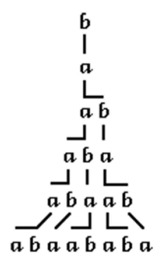
The L-System has been introduced by Aristid Lindenmayer in the late 1960s to describe the growth of spatial systems such as cells or plants [19]. Basically, an L-System consists of a string containing different letters and numbers which are used to either execute a specific turtle-based drawing operation in 2D or 3D space or to re-orientate the turtle in space or store and restore its position.

An L-System is a rewriting system that can contain rules for replacing letters with other letters or sequences of letters in each re-writing step. The replaced letters are inserted into the existing L-String and they are also subject to replacement in the next re-writing step, hence, generating a fractal-like sequence.

Figure 1 shows the development of an L-System with the following properties:

• Start term (Axiom): b
• Replacement Rule 1: b → a
• Replacement Rule 2: a → ab

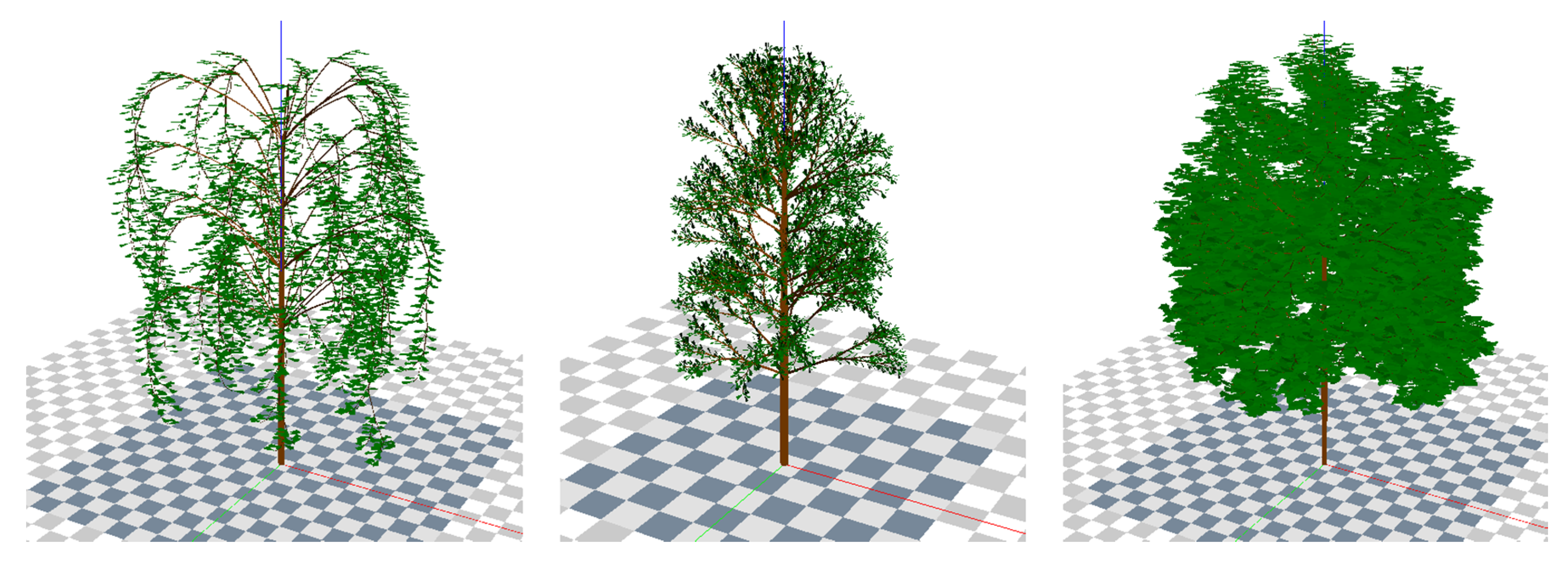
Figure 2 shows three different tree species generated with the L-System. Using the L-System skeleton, the LAD cluster is then derived, depending on the actual model areal resolution.

The placement of leaves can be controlled by the user over a wide range of parameters, including leaf size, orientation, and positioning.

The software allows a wider range of settings to control the leaf placement including the internode length, leaf positioning, and phyllotaxis angels. Moreover, the geometry of the leaf can be set by the user to generate species-depending leaf types.

In every stage of the tree generation, the biomechanics of the tree are calculated and considered in the tree skeleton geometry. For each branch segment (typically 0.2 m), the torques generated through the self-loading of the attached child segments are set in correlation to the tree’s basic mechanical properties such as Young’s modulus to estimate the deformation and rotation of each tree segment.

The final tree skeleton is obtained, when all generated torques and the internally stored energy in the tree segment through deformation and rotation are balanced. If the user designs a tree which is biomechanically instable from the beginning, it is rejected by ENVI-met.

To use the new Lindenmayer-based trees (L-Trees) in ENVI-met, the leaf location rasterized in the usual 1 × 1 × 1 m grid and the associated Leaf Area Density for each grid is calculated by summing up the leaf surface inside the assigned grid box.

2.2. Advancements in the ENVI-met Canopy Radiation Model

Extinction of shortwave radiation in ENVI-met is handled using a ray tracing algorithm [20]:

In the ray trace, each cell shoots a linear ray in a predefined direction and checks for obstructions along its way through a three-dimensional space.

The ray tracing is implemented using an iterative approach:

$$\mathrm{p}\left(\mathrm{x},\mathrm{y},\mathrm{z},\mathrm{n}+1\right)=\mathrm{p}\left(\mathrm{x},\mathrm{y},\mathrm{z},\mathrm{n}\right)+\mathsf{\lambda }\mathrm{v}$$

(1)

with $\mathrm{p}\left(\mathrm{x},\mathrm{y},\mathrm{z},\mathrm{n}\right)$ as the point of the ray at iteration $n$ and λv as a three-dimensional vector heading towards a certain position described by an azimuthal and elevation angle. The λv vector’s length is sized depending on the grid cell resolution and direction angle to ensure that grid cells which lie substantially on the ray’s path are actually hit at each iteration.

Depending upon the objects (building, single wall, terrain, vegetation) that lie in the ray’s path, a local transmission factor $({\mathrm{f}}_{\mathrm{Obj}}\left(\mathrm{i},\mathrm{j},\mathrm{k}\right)$) ranging from 0 to 1 is obtained. While the ray continues on its way, a product of all individual local transmission factors iteratively forms the total transmission factor (${\mathrm{f}}_{\mathrm{tot}}$) of the starting grid cell in the ray’s direction:

$${\mathrm{f}}_{\mathrm{tot}}\left(\mathrm{n}+1\right)={\mathrm{f}}_{\mathrm{tot}}\left(\mathrm{n}\right){\ast \mathrm{f}}_{\mathrm{Obj}}\left(\mathrm{i},\mathrm{j},\mathrm{k}\right)$$

(2)

Different objects carry different transmission factors (${\mathrm{f}}_{\mathrm{Obj}}\left(\mathrm{i},\mathrm{j},\mathrm{k}\right)$). For direct shortwave radiation, buildings and ground surfaces carry a transmission factor of 0. For single walls, the material’s transmission is taken as the object’s transmission factor. To calculate the transmission of direct and diffuse shortwave radiation through vegetation grids, i.e., the attenuation of direct and diffuse shortwave radiation, new approaches following the works of Pedruzo-Bagazgoitia et al., 2017 [21] have been implemented. The new scheme tries to model the processes of shortwave radiation in canopies using three processes:

• Primary extinction of direct shortwave radiation.
• Extinction of direct shortwave radiation due to scattering and creation of secondary diffuse shortwave radiation.
• Extinction of diffuse shortwave radiation.

2.2.1. Primary Extinction of Direct Shortwave Radiation

Primary extinction of direct radiation is modelled using an extinction coefficient depending on solar elevation [25,26]:

$${\mathrm{k}}_{\mathrm{dirbl}}=\frac{0.5}{\sin \mathsf{\beta }}$$

(3)

with $\mathsf{\beta }$ as the solar elevation angle above the horizon. Since the primary extinction of direct radiation only accounts for the pure extinction of direct radiation, leaves are considered visually black—thus neither transmitting nor reflecting, only absorbing direct radiation [25,26].

The transmission factor for primary extinction of direct radiation is then calculated using a ray tracing for every grid in the direction of the sun’s position. When hitting a plant grid cell, the local transmission factor is calculated by:

$$\begin{array}{c}{\mathrm{f}}_{\mathrm{Veg},\mathrm{dir},\mathrm{pri}}\left(\mathrm{i},\mathrm{j},\mathrm{k}\right)=\\ \left(1-{\mathsf{\rho }}_{\mathrm{dir}}\right)\ast \left(1-\mathsf{\sigma }\right)\ast {\mathrm{e}}^{-\left({\mathrm{k}}_{\mathrm{dirbl}} \mathrm{LAIc}\right)}\end{array}$$

(4)

with $LAIc$ as the sum of Leaf Area Index (LAI) between the grid cell and the sun’s position on the ray’s path and ${\mathsf{\rho }}_{\mathrm{dir}}$ as a sun elevation dependent reflection coefficient of direct radiation on horizontally distributed leaves. As the actual amount of horizontally orientated leaves is unknown, the model considers a leaf angle distribution of 0.5—representing an average horizontal orientation of 50% of the leaves [17,25]:

$$\mathsf{\rho } =\frac{1-\sqrt{1-\mathsf{\sigma }}}{1+\sqrt{1-\mathsf{\sigma }}}$$

(5)

$${\mathsf{\rho }}_{\mathrm{dir}}=\mathsf{\rho } \frac{2}{1+1.6 \sin \mathsf{\beta }}$$

(6)

After calculating the local transmission factor, the total transmission factor is updated (see Equation (2)) and the ray tracing continued until the termination condition of the ray tracing is reached. The direct shortwave radiation of grid cell $\mathrm{i},\mathrm{j},\mathrm{k}$ is then calculated by:

$${\mathrm{Q}}_{\mathrm{dir}}\left(\mathrm{i},\mathrm{j},\mathrm{k}\right)={\mathrm{Q}}_{\mathrm{dir},\mathrm{top}}{\ast \mathrm{f}}_{\mathrm{tot},\mathrm{dir},\mathrm{pri}}$$

(7)

with ${\mathrm{Q}}_{\mathrm{dir},\mathrm{top}}$ as the incoming direct shortwave radiation at model top and ${\mathrm{f}}_{\mathrm{tot},\mathrm{dir},\mathrm{pri}}$ as the total transmission factor handling the extinction of radiation within plant canopies according to Equation (4).

2.2.2. Extinction of Direct Shortwave Radiation Due to Scattering of Direct Radiation and Creation of Secondary Diffuse Radiation

To account for creating secondary diffuse radiation due to scattering of direct radiation, the extinction coefficient ${\mathrm{k}}_{\mathrm{dirbl}}$ is altered using an empirical constant $\mathsf{\sigma }$ accounting for scattering of direct shortwave radiation in the vertical direction [25,26]:

$${\mathrm{k}}_{\mathrm{dir}}={\mathrm{k}}_{\mathrm{dirbl}}\ast \sqrt{1-\mathsf{\sigma }}$$

(8)

The transmission factor for extinction of direct shortwave radiation due to scattering and by that creating secondary diffuse radiation is calculated using a ray tracing of every grid cell towards the sun’s position. Upon hitting a plant grid cell, the transmission is, following the works of Pedruzo-Bagazgoitia et al., 2017, then calculated as follows:

$${\mathrm{f}}_{\mathrm{Veg},\mathrm{dir}+\mathrm{dif},\sec }\left(\mathrm{i},\mathrm{j},\mathrm{k}\right)=\left(1-{\mathsf{\rho }}_{\mathrm{dir}}\right){\ast \mathrm{e}}^{-\left({\mathrm{k}}_{\mathrm{dir}} \mathrm{LAIc}\right)}$$

(9)

The resulting transmission factor incorporates the sum of the processes of extinction of direct shortwave radiation and creation of secondary diffuse radiation [21]. Thus, after the ray tracing is terminated, the net creation of secondary diffuse radiation can be calculated in two steps:

Firstly, the combined extinction of direct shortwave radiation and creation of secondary diffuse radiation is calculated by multiplying the total transmission factor with the incoming direct shortwave radiation at model top:

$${\mathrm{Q}}_{\mathrm{dir}+\mathrm{dif},\sec }\left(\mathrm{i},\mathrm{j},\mathrm{k}\right)={\mathrm{Q}}_{\mathrm{dir},\mathrm{top}}{\ast \mathrm{f}}_{\mathrm{tot},\mathrm{dir}+\mathrm{dif},\sec }$$

(10)

with ${\mathrm{f}}_{\mathrm{tot},\mathrm{dir}+\mathrm{dif},\sec }$ as the total transmission factor handling the extinction of radiation within plant canopies according to Equation (10).

Secondly, the previously calculated primary extinction of only direct radiation is subtracted from the combination of direct radiation’s extinction and secondary diffuse radiation’s creation due to scattering. The net creation of secondary diffuse radiation is thus:

$${\mathrm{Q}}_{\mathrm{dif},\sec }\left(\mathrm{i},\mathrm{j},\mathrm{k}\right)={\mathrm{Q}}_{\mathrm{dir}+\mathrm{dif},\sec }\left(\mathrm{i},\mathrm{j},\mathrm{k}\right)-{\mathrm{Q}}_{\mathrm{dir}}\left(\mathrm{i},\mathrm{j},\mathrm{k}\right)$$

(11)

2.2.3. Extinction of Diffuse Shortwave Radiation

The extinction coefficient of diffuse radiation (${\mathrm{k}}_{\mathrm{dif}}$), however, is quite similar to the extinction coefficient ${\mathrm{k}}_{\mathrm{dir}}$. Since diffuse radiation is considered isotropic, sun angle dependency is neglected and replaced by a constant factor of 0.8 [21]:

$${\mathrm{k}}_{\mathrm{dif}}=0.8\ast \sqrt{1-\mathsf{\sigma }}$$

(12)

While Pedruzo-Bagazgoitia et al., 2017 [21] suggested calculating the extinction of diffuse radiation only for a vertical column, i.e., a ray trace perpendicular to a horizontal surface, a more realistic approach using a hemispherical ray tracing is applied to account for the isotropic nature of diffuse radiation in the model.

Other than in the ray tracing for the direct radiation (see above), the ray trace for diffuse extinction is not directed towards the sun’s position, but in all directions of the upper hemisphere of a cell with angular distances of 5° height and 10° azimuthal angle:

$$\mathsf{\lambda }\mathrm{v}=\left(\begin{array}{c}\overline{\mathrm{v}}\ast \cos \left(\mathrm{h}\right)\ast \cos \left(\mathrm{a}\right)\\ \overline{\mathrm{v}}\ast \cos \left(\mathrm{h}\right)\ast \sin \left(\mathrm{a}\right)\\ \overline{\mathrm{v}}\ast \sin \left(\mathrm{h}\right)\end{array}\right)$$

(13)

with λv as a three-dimensional ray tracing vector, $\overline{\mathrm{v}}$ as the vector length, $\mathrm{a}$ as the azimuthal, and $\mathrm{h}$ as the height angle of the ray.

For each ray an individual transmission factor is calculated:

$${\mathrm{f}}_{\mathrm{Veg},\mathrm{dif},\mathrm{pri}}\left(\mathrm{i},\mathrm{j},\mathrm{k}\right)=\left(1-\mathsf{\rho }\right){\ast \mathrm{e}}^{-\left({\mathrm{k}}_{\mathrm{dif}} \mathrm{LAIc}\right)}$$

(14)

The resulting individual transmission factors for every ray trace are then averaged to gain the overall transmission factor for diffuse radiation.

Since the transmission factor of diffuse shortwave radiation extinction does not depend on the current solar elevation, it can be precalculated during the initialization phase of the model and stored in a three-dimensional array. It only needs updating after user-defined intervals (Figure 3) to account for changes in the local LAD of deciduous vegetation, i.e., leaf shedding.

The extinction of diffuse shortwave radiation is then calculated by:

$${\mathrm{Q}}_{\mathrm{dif}}\left(\mathrm{i},\mathrm{j},\mathrm{k}\right)={\mathrm{Q}}_{\mathrm{dif},\mathrm{top}}{\ast \mathrm{f}}_{\mathrm{tot},\mathrm{dif},\mathrm{pri}}$$

(15)

with $Q_{dif,top}$ as the incoming diffuse shortwave radiation at model top.

The total diffuse radiation in grid cell $i,j,k$ is then calculated as the sum of extinct diffuse shortwave radiation and secondary diffuse radiation created by scattering of direct radiation:

$${\mathrm{Q}}_{\mathrm{dif},\mathrm{tot}}\left(\mathrm{i},\mathrm{j},\mathrm{k}\right)={\mathrm{Q}}_{\mathrm{dif}}\left(\mathrm{i},\mathrm{j},\mathrm{k}\right)+{\mathrm{Q}}_{\mathrm{dif},\sec }\left(\mathrm{i},\mathrm{j},\mathrm{k}\right)$$

(16)

2.2.4. Enabling/Disabling the Advanced Canopy Transfer Module

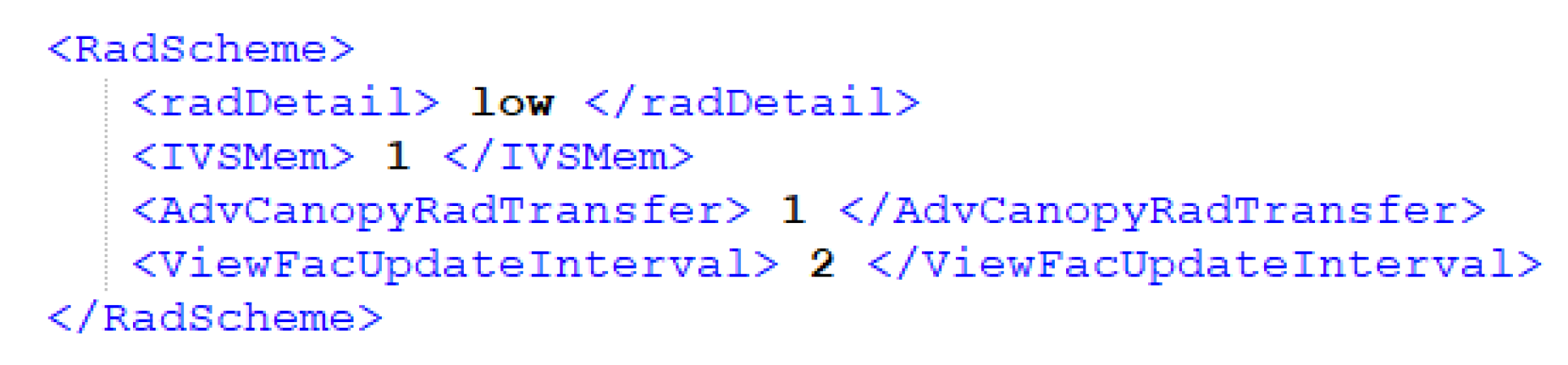
The advanced canopy radiation transfer module can be enabled in the simulation settings of the SIMX file. By default, the module is switched off. If enabled, the user is able to adjust the interval at which the transmission factor analysis is updated. The update interval accounts for effects of leaf shedding onto the radiation calculation. It only takes effect for longer simulation periods when deciduous plants adapt to the environment by shedding their leaves—its value is given in days.

The controlling tags on the SIMX-File are in section RadScheme under AdvCanopyRadTransfer and ViewFacUpdateInterval (Figure 3). Both tags can be edited individually since the update of the ViewFacUpdateInterval also controls the update interval of the view factors analysis.

In case the ACRT module is disabled, the extinction of direct shortwave radiation is carried out as in previous versions of ENVI-met:

$${\mathrm{f}}_{\mathrm{veg}}\left(\mathrm{i},\mathrm{j},\mathrm{k}\right)={\mathrm{e}}^{-\left(\mathsf{\omega }\ast \left(1-\mathrm{t}\right)\ast \mathrm{LAD}\left(\mathrm{i},\mathrm{j},\mathrm{k}\right)\ast \left|\mathsf{\lambda }\mathrm{v}\right|\right)}$$

(17)

with $\mathsf{\omega }$ as the leaf orientation, constant at 0.5, $\mathrm{t}$ as the shortwave transmittance of the leaves, $\mathrm{LAD}\left(\mathrm{i},\mathrm{j},\mathrm{k}\right)$ as the local leaf area density, and $\left|\mathsf{\lambda }\mathrm{v}\right|$ as the length of the current ray segment. The three-dimensional array containing the secondary diffuse radiation is set to 0 and the function calculating the extinction coefficient of diffuse radiation only returns the local sky view factor. This way, the resulting transmission for direct and diffuse shortwave radiation remains identical to previous versions.

2.3. Proof-of-Concept Simulation

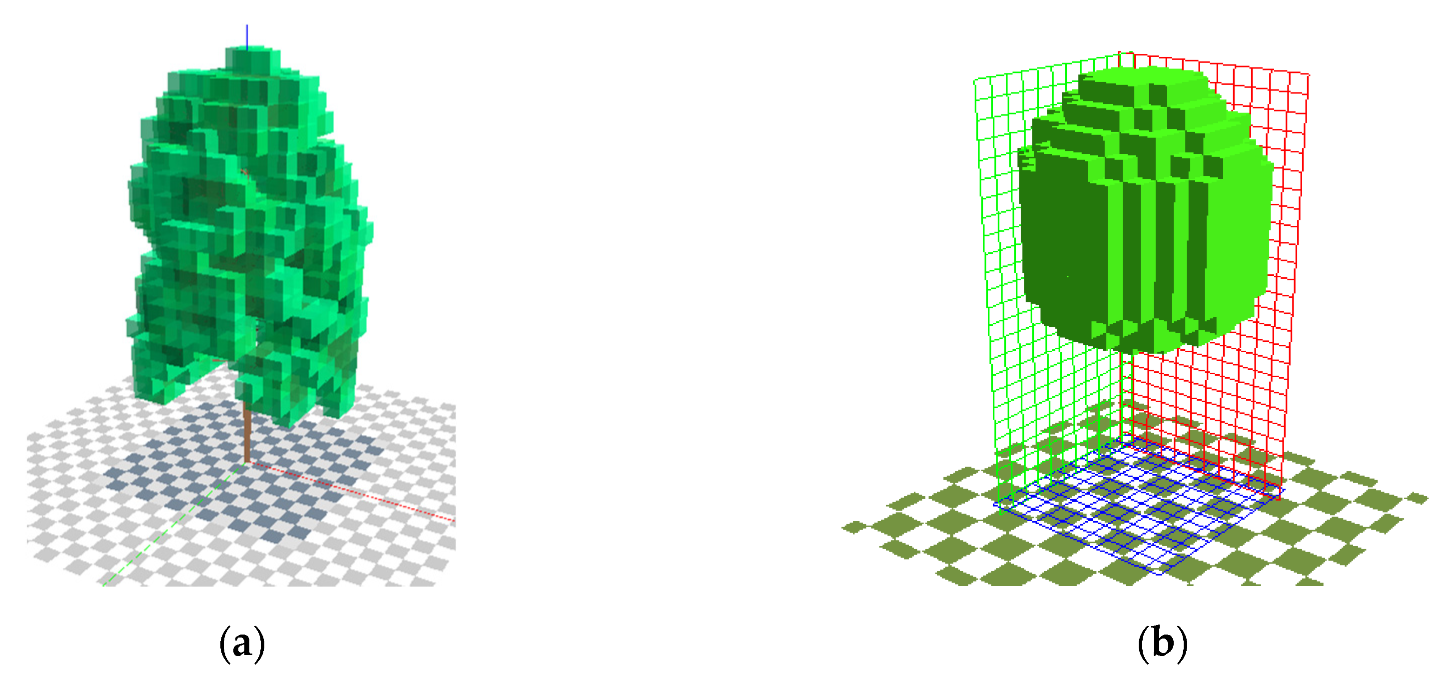
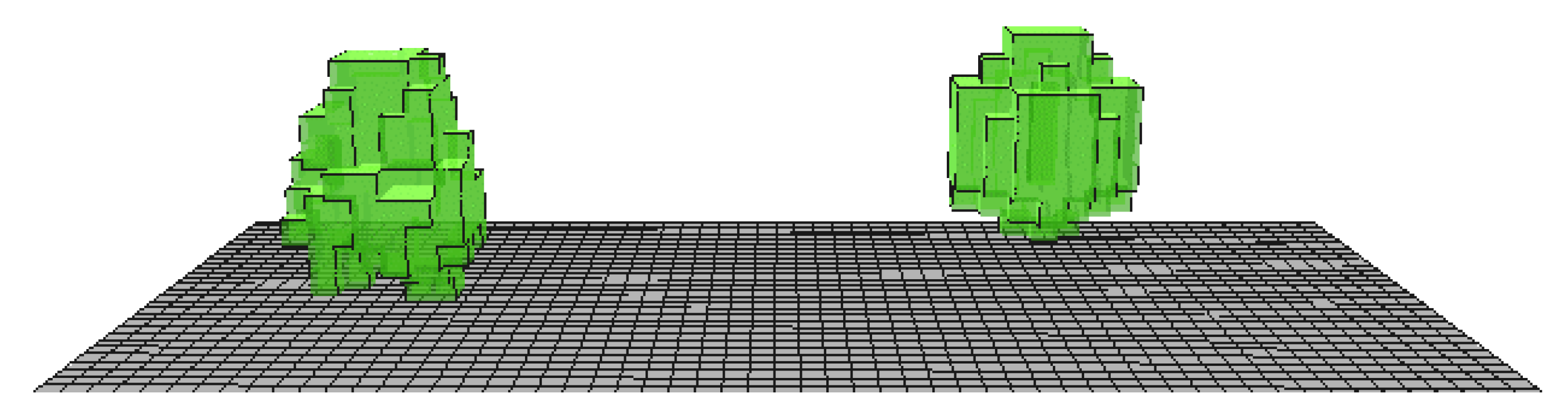
In a small model area featuring a standard solid Parametric-Tree and its L-Tree resemblance, the advancements of the algorithmic plant generation and the advanced canopy radiation transfer module is evaluated (Figure 4 and

Table 1. Parameters of Parametric-Tree and L-Tree.

	Height (m)	Diameter (m)	LAD (m2/m3)	Total Leaf Area (m2)	Number of LAD Cells
L-Tree	25	11	0.025–0.825 1	298.36	222
Parametric-Tree	25	11	0.3	460.8	192

¹ LAD varies as it is created based on the leaf setting rule set.

). The trees have been modelled to resemble a Balsam poplar with a height of 25 m as this species features a very heterogenous LAD distribution.

It is to be expected, that the L-Tree, due to its realistic LAD clusters, shows more diverse radiation patterns of direct shortwave radiation. In combination with the advanced canopy radiation transfer module, not only the extinction of diffuse radiation and creation of secondary diffuse radiation should be more realistic, but also the photosynthetic activity and thus leaf temperatures as well as latent heat flux.

The model area consists of 100 × 70 × 40 grid cells in a resolution of 2 × 2 × 2 m and is located in Essen, Germany, thus representing a typical location in Central Europe with Cfb climate in the Köppen-Geiger classification (Figure 5).

To evaluate the effects of the ACRT module, a second simulation run with the module switched off has been conducted. The simulation has been run for 24 h starting from June 23rd at 05:00 h. The meteorological boundary conditions were set using a simple forcing for a warm summer day with no cloud cover.

The model results are first compared against each other and subsequently against literature values of similar trees. Finally, the impact on thermal comfort underneath the trees is compared between the simulation runs.

3. Results and Discussion

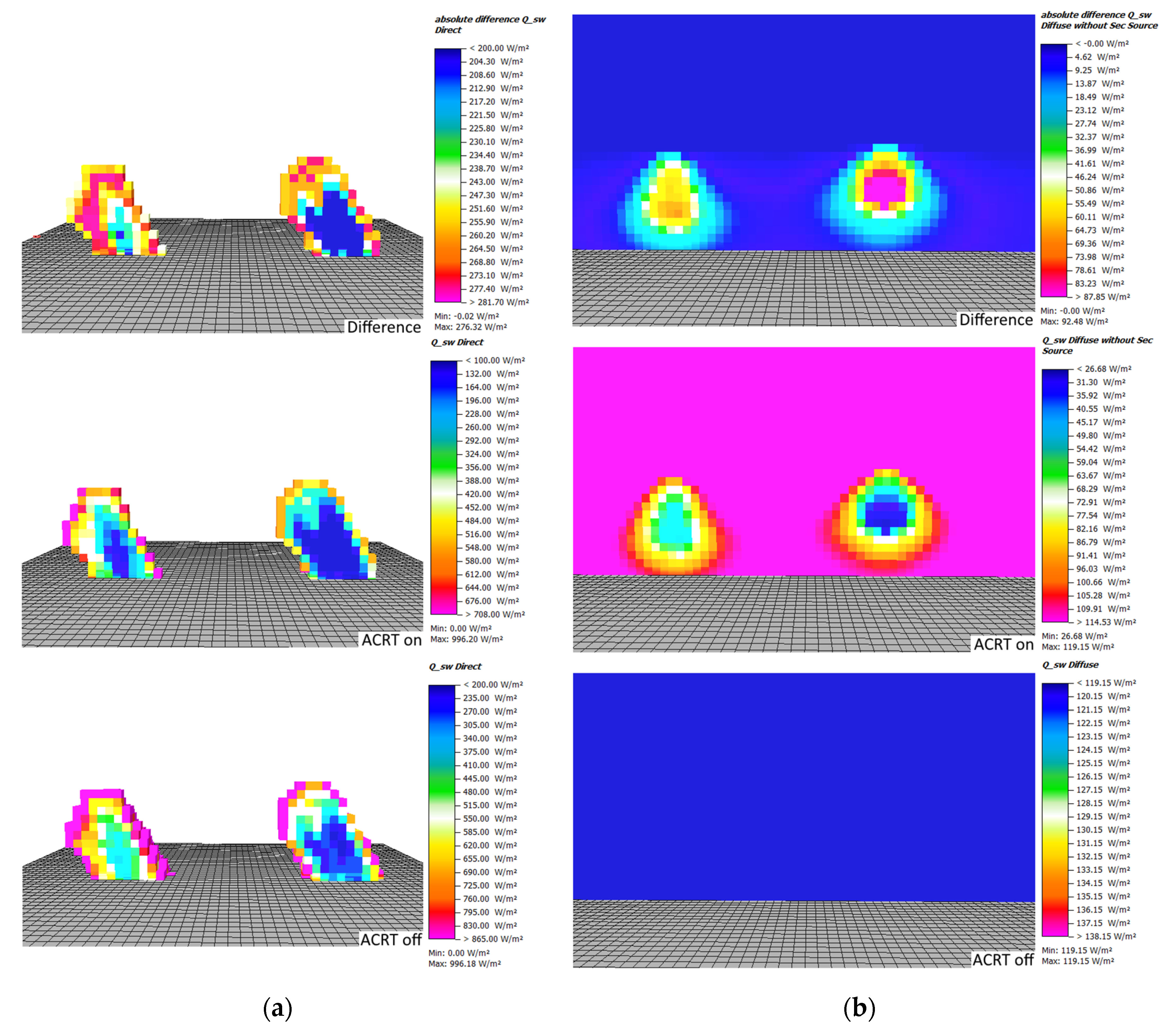
To visualize the effects of the advancements of L-Trees and the ACRT module onto the microclimate results, maps showing the absolute values of direct and diffuse radiation as well as difference maps for the two simulation runs have been created. In the difference maps, positive values indicate lower values in the simulation including the ACRT module.

By looking at the differences in direct and diffuse shortwave radiation between the two simulations at noon, the total effect of the L-Trees and the ACRT module can be seen (Figure 6).

A vertical cut along the centerline of the trees reveals that, for the direct shortwave radiation, the highest reduction occurs at the top of the canopy for both trees. However, the reduction of direct shortwave radiation within the Parametric-Tree canopy is much greater due to its homogenously distributed high LAD. For the L-Tree, the reductions occur more gradually as its LAD is lower on average than the Parametric-Tree’s LAD. Both trees show greater extinction of direct shortwave radiation with the ACRT module on. While the inner canopy direct shortwave radiation only drops to a minimum of around 150 W/m² for the L-Tree in the ACRT on simulation, the solid structure of LAD in the center of the Parametric-Tree leads to a massive and rather unrealistic reduction of the direct shortwave radiation: In both simulations, with and without the ACRT module, the direct shortwave radiation completely gets extinct in the inner canopy of the Parametric-Tree.

The comparison of diffuse radiation at noon in Figure 6 shows that with the ACRT module, no diffuse shortwave radiation is attenuated in the tree canopies. The result of the ACRT simulation clearly shows the isotropic character of diffuse radiation as the distribution of diffuse radiation is independent on the sun’s position. Similarly, to the extinction of direct shortwave radiation, the attenuation of diffuse radiation is greater in the Parametric-Tree (down to around 26 W/m²) compared to the L-Tree (50 W/m²) (Figure 6).

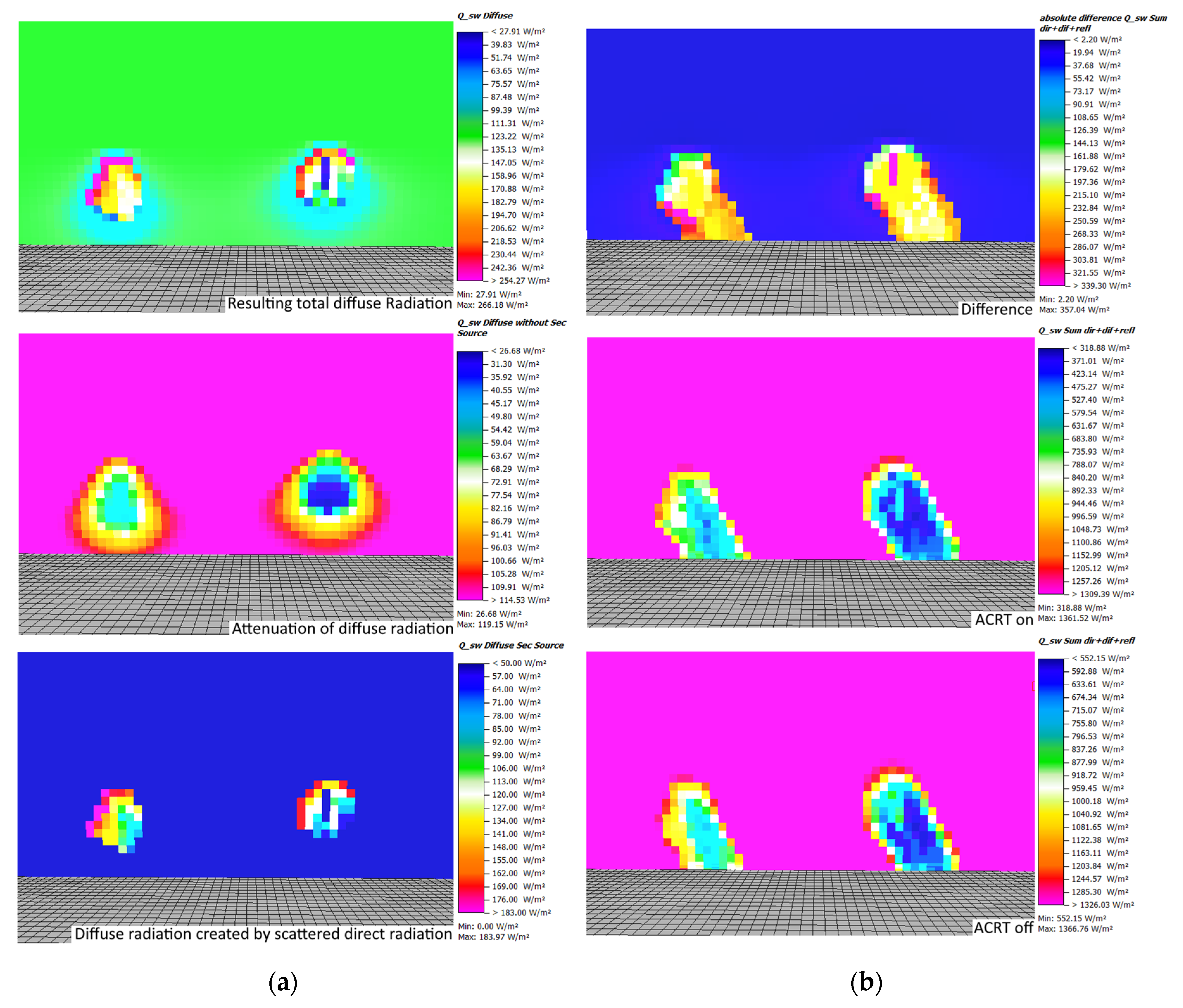
Since diffuse radiation is also created by scattering of direct shortwave radiation when ACRT is on, the results for diffuse radiation in Figure 7 do not show the total inner canopy diffuse radiation. The amount of diffuse radiation created by scattering of direct radiation (secondary source of diffuse radiation) can be seen in Figure 7a. Similar to the direct radiation, more diffuse radiation is created at the outer canopy. In a comparison between both trees, more secondary diffuse radiation is found within the L-Tree’s canopy, as direct radiation penetrates deeper inside the L-Tree resulting in more available direct shortwave radiation to be scattered (see above).

Looking at the sum of all shortwave fluxes (direct, diffuse, and reflected radiation), the increased extinction of direct radiation—and in case the ACRT module is on also the extinction of diffuse shortwave and the lower creation of secondary diffuse radiation—in the Parametric-Tree leads to significantly lower total shortwave radiation values compared to the L-Tree (around 200 W/m² difference). The effect of ACRT accounts for an additional 200 W/m² difference between both trees, resulting in inner canopy values for the L-Tree of around 550 W/m² with the ACRT module and 750 W/m² without the ACRT module. For the Parametric-Tree, the difference is very similar, with 330 W/m² with the ACRT module and 550 W/m² without the ACRT module.

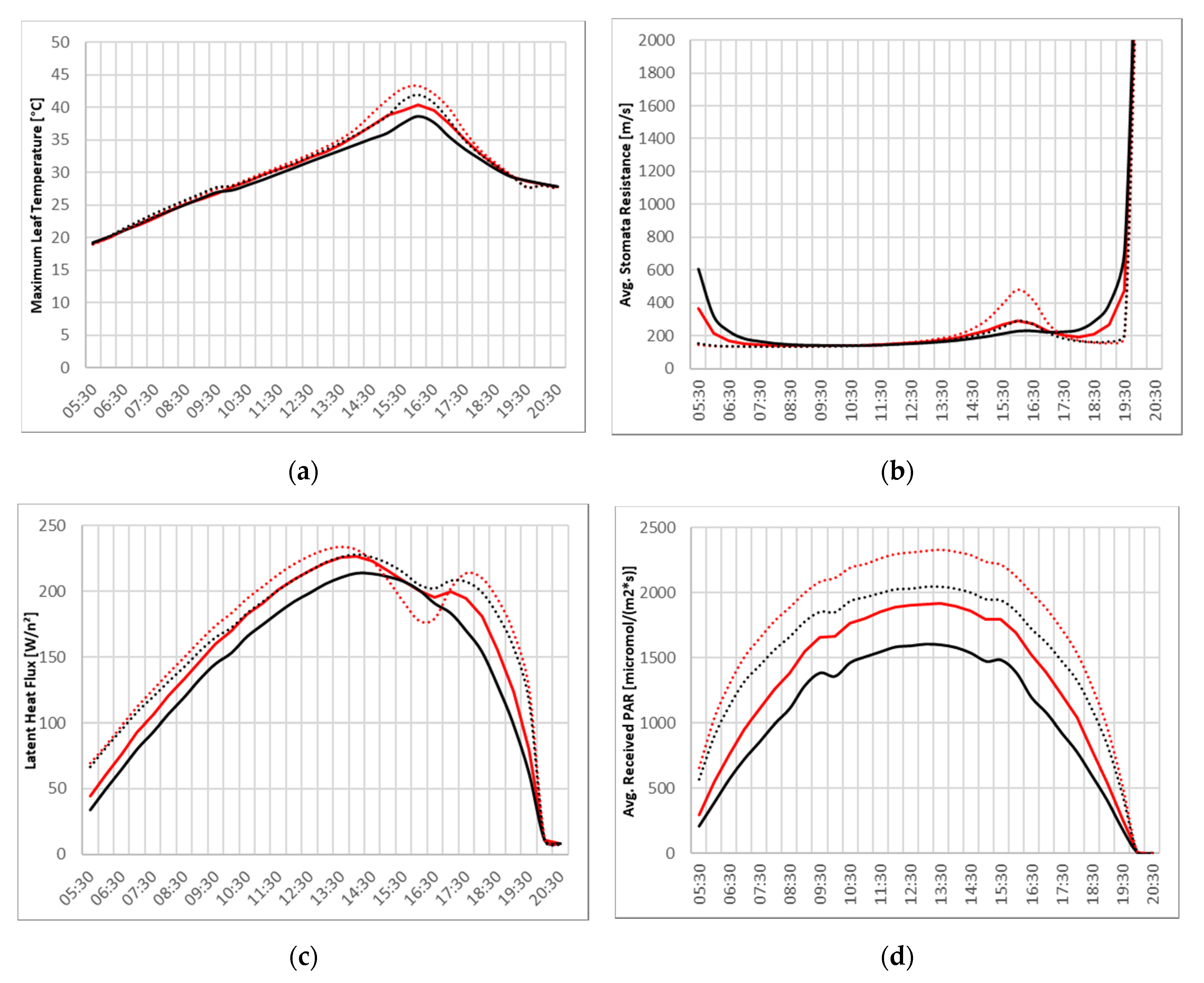
Since different inner canopy radiation patterns lead to alterations in plant physiology of the trees, several indicators for the tree’s behavior have been analyzed for the photosynthetic active hours, i.e., day light hours of the simulation (Figure 8).

The diurnal cycles of maximum leaf temperature, average stomata resistance, latent heat flux, and average received photosynthetic active radiation (PAR) show large differences of the two trees and with and without the ACRT module.

Maximum leaf temperatures show rather similar values until the afternoon, after which the trees in the simulation without ACRT experience significantly higher maximum leaf temperatures (>40 °C) indicating thermal stress. This can also be seen in the sudden spike in average stomata resistance of the trees in the ACRT off simulations. The increased stomata resistance leads to lower vapor fluxes which in turn reduces latent heat flux and increases leaf temperatures. Additionally notable, is the less sudden drop of the stomata resistance in the morning and the sudden drop of the stomata resistance in the evening for the ACRT on simulations. This is caused by the introduction of attenuation of diffuse radiation, which leads to a more gradual progression in the morning and evening hours.

The curve of average received PAR corroborates the inner canopy radiation analyses at noon above, with highest values for the L-Tree in the ACRT off simulation and lowest values for the Parametric-Tree in the ACRT on simulation.

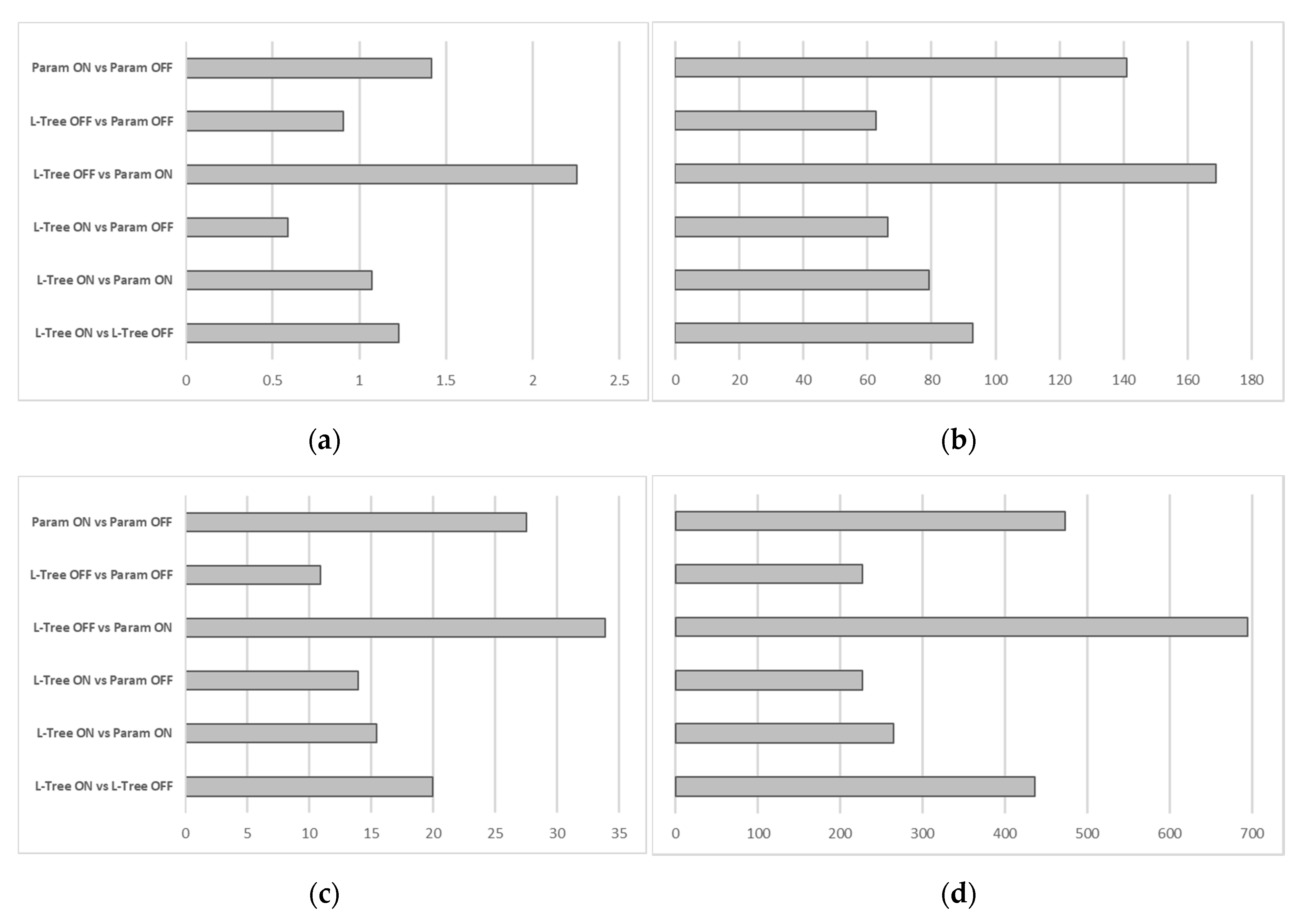
In order to entangle the contributions of the advancements of the L-Tree and the ACRT module, Root Mean Square Errors (RSME) between different combinations of Parametric-Tree, L-Tree, and ACRT on and ACRT off simulations have been calculated for maximum leaf temperature, average stomata resistance, latent heat flux, and average received photosynthetic active radiation (Figure 9).

The comparison of the Root Mean Square Errors shows the same general tendencies for all parameters. The biggest differences occur between the L-Tree without the ACRT module and the Parametric-Tree with the ACRT module. This indicates that the advancements of the ACRT module and the L-Tree complement each other, as their combination leads to the highest values of RMSE. Looking at the isolated effects of the L-Tree and the ACRT advancements, it seems, that the ACRT module (comparison between Parametric-Tree with ACRT and Parametric-Tree without ACRT) has a slightly greater effect for all parameters than the equivalent isolated L-Tree advancements (comparison between L-Tree without ACRT and Parametric-Tree without ACRT). The largest effect when only enabling one advancement can be seen in the combination of Parametric-Tree and ACRT on/off. This indicates, that by only enabling the ACRT module, the parameters of maximum leaf temperature, average stomata resistance, latent heat flux, and average received photosynthetic active radiation match the supposedly most realistic simulation featuring an L-Tree with the ACRT module rather closely already. This suggests that the ACRT module has a greater impact onto the plant specific parameters, while the L-Tree implementation alone also constitutes further advancements, their isolated effects seem to have a lesser extent onto the parameters shown.

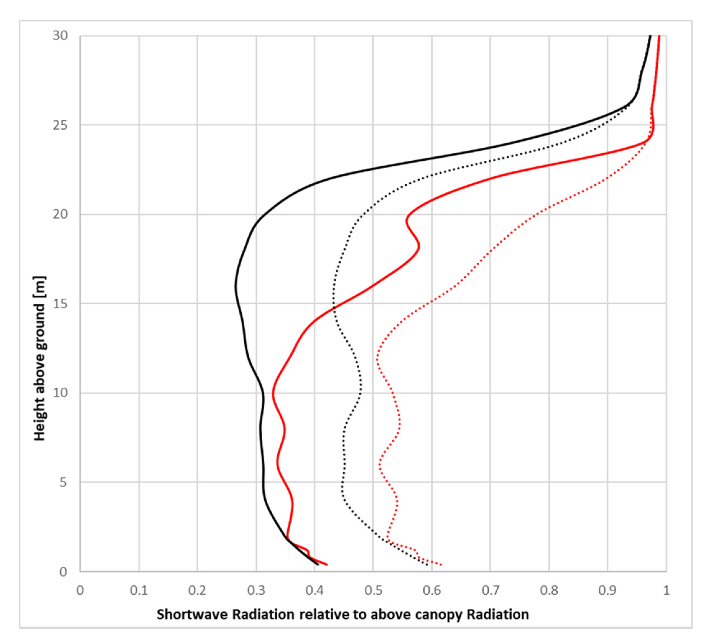
The vertical distribution of shortwave radiation within the canopy of all combinations shows a steep decline with decreasing height, most pronounced in ACRT on simulations (Figure 10). While the Parametric-Tree with its homogenous LAD structure shows an almost steady decline in the ACRT on simulations, the L-Tree’s shortwave radiation reduction varies in its strength. Values at ground level for the ACRT on simulation are, however, similar with around 40%. In contrast, both trees show a less pronounced decline of shortwave radiation in the ACRT off simulation, mainly because diffuse radiation is not attenuated without the ACRT module. The resulting ground level shortwave radiation for the ACRT off simulation lies around 60% for both trees.

Comparing these results with literature values for similar trees (regarding height and LAD), such as Balsam poplar in Mixlight where the authors compared predicted inner canopy radiation transmittance against measured values, shows that the simulation of the L-Tree with the ACRT module matches the measured and modelled values of Mixlight quite closely [27]. Other literature values of, e.g., Thakur and Kaur, 2001 [28] or Bartelink, 1998 [29] come to slightly lower ground level values of around 10% to 20%, however, featuring denser trees. Further direct comparison with literature values is constrained, as most studies are carried out on trees in forest stands instead of isolated locations [30,31].

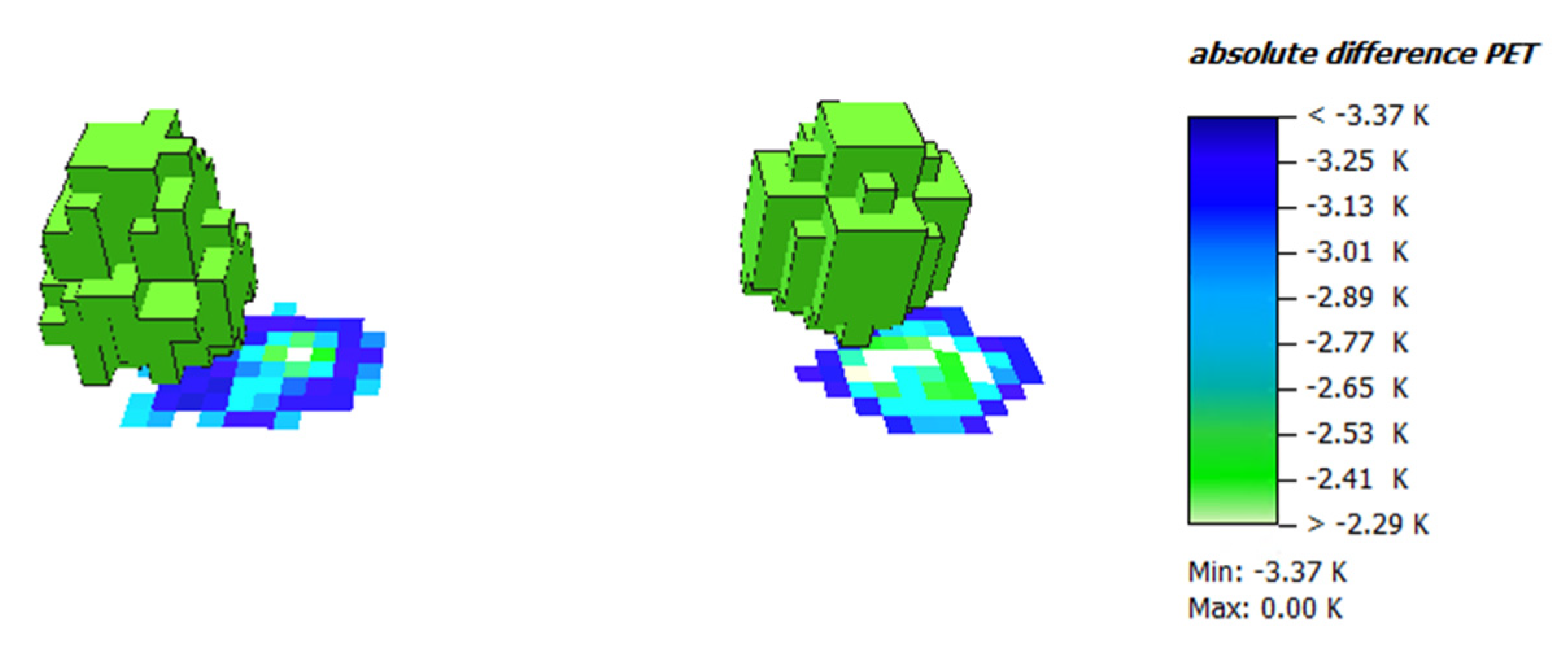
To examine the effect of both advancements onto the thermal comfort, the Physiological Equivalent Temperature (PET) underneath both trees has been calculated in a height of 1.4 m (Figure 11). The results show generally lower PET values in the ACRT including simulations of around 2 to 3.37 K for both trees. While the PET pattern underneath the parametric tree shows a more homogenous reduction of PET, the PET underneath the L-Tree is heterogeneously distributed as the non-uniform LAD clusters of the L-Tree cause different levels of shading and thus mean radiant temperature.

4. Conclusions

This contribution presents a combined effort to improve the modelling of the microclimate effect of trees on the one hand and plant vitality parameters on the other. By developing a sophisticated plant digitalization method enabling the much more realistic description of plants, the microclimate important position and alignment of leaf clusters can be deduced. Further advancements of the inner canopy radiation scheme enabling the attenuation of diffuse radiation and the creation of secondary diffuse radiation by scattering of direct radiation, lead to much more diverse radiation patterns inside and around the plant. In two proof-of-concept simulations, the effects of the advancements were examined regarding the radiative scheme as well as different plant physiological and microclimatic parameters. The results showed significant differences between the tree types as well as the radiative transfers. It can be expected that, with the new advancements, modelling of microclimate effects of trees and plant vitality is considerably improved. Samples from literature values seem to corroborate this finding. However, since no empirical tests have been undertaken yet, the strength of the new approaches needs to be evaluated in real case scenarios. Due to parallelization, the simulation time is not significantly affected by including L-Trees or the ACRT module and can thus be used in larger, more complex model areas as well.

Results of the thermal comfort beneath the trees showed significant differences in PET as the shading and thus the mean radiant temperature is greatly affected by the new radiation scheme as well as the non-uniform LAD distribution of the L-Trees. This indicates that the use of both advancements will yield a better understanding of not only the plant physiological parameters, but also the effects of trees onto the local microclimate. Future developments of both modules should address the translation of the branching system into the radiative simulation to account for effects such as absorption of shortwave radiation by the branches as well. Furthermore, the inclusion of branches should make plant biomechanical simulations possible predicting the probability of branch failure due to wind gusts.