Key Elements of the White-Backed Woodpecker’s (Dendrocopos leucotos lilfordi) Habitat in Its European South-Western Limits

 , ,
, ,
Abstract
:1. Introduction
2. Materials and Methods
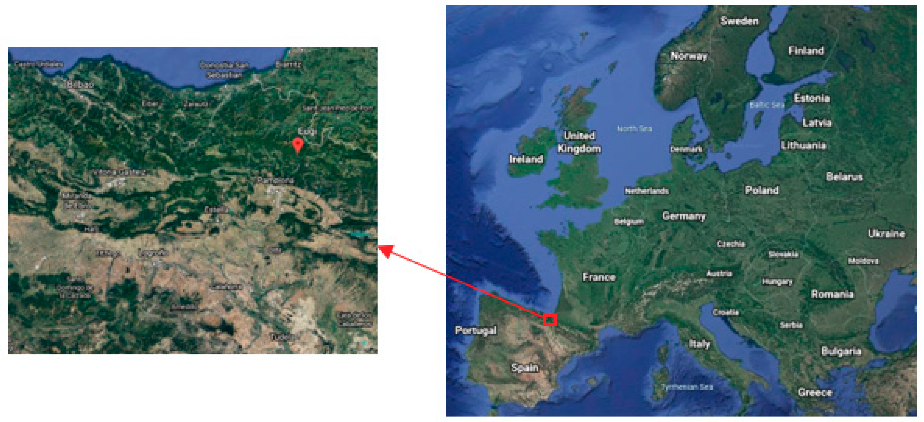
2.1. Study Area
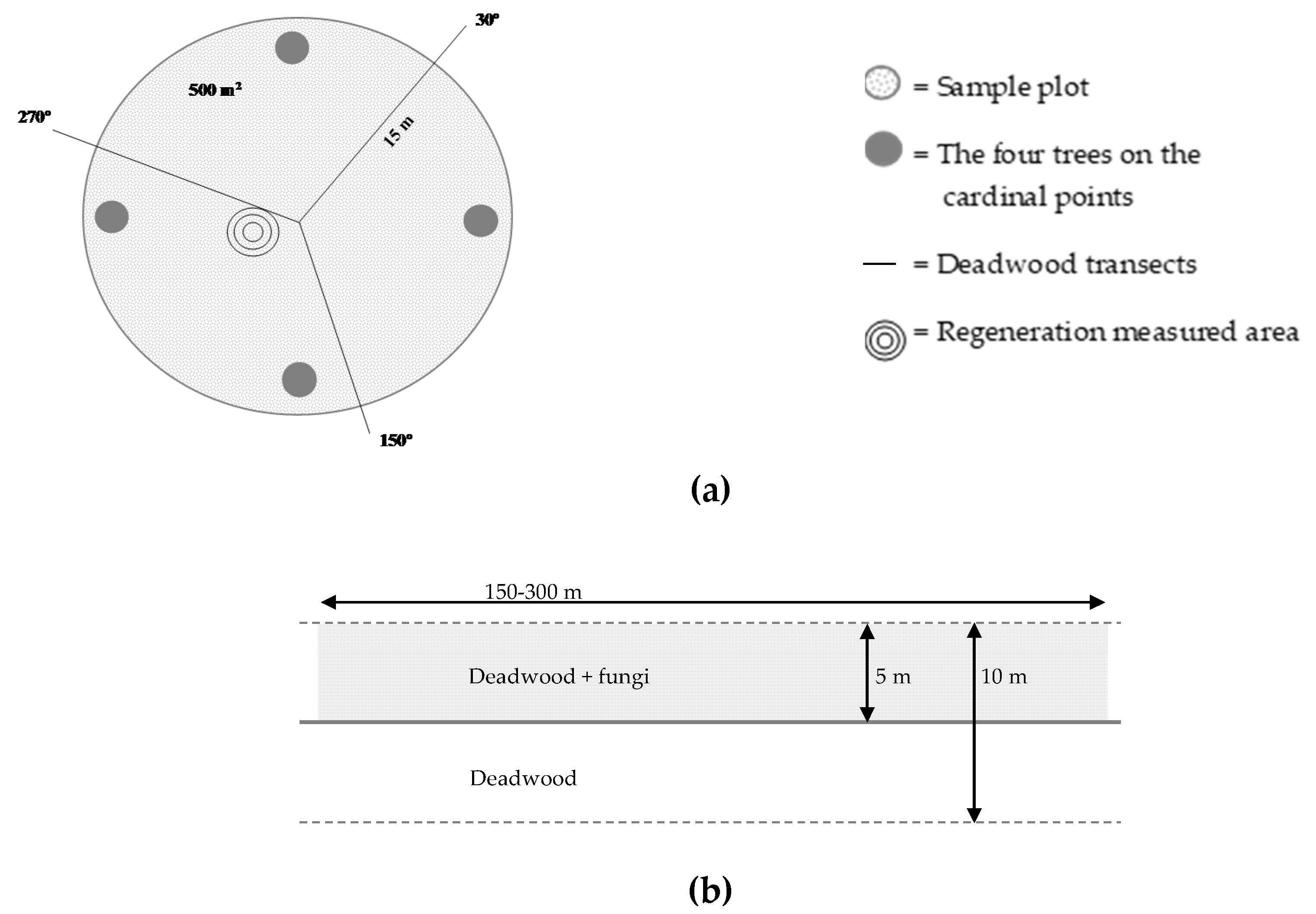
2.2. Sampling Methodology
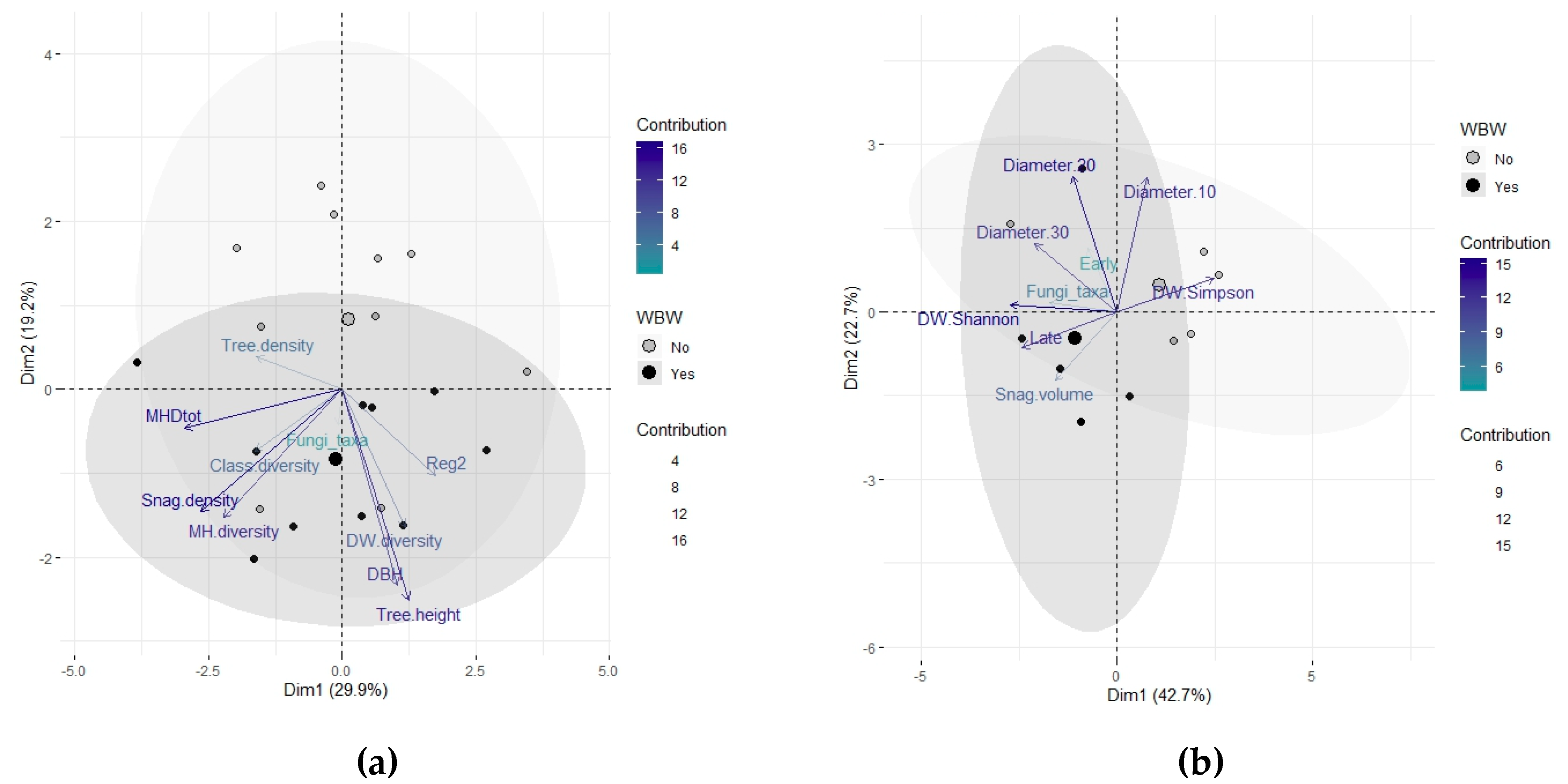
2.3. Data Analysis
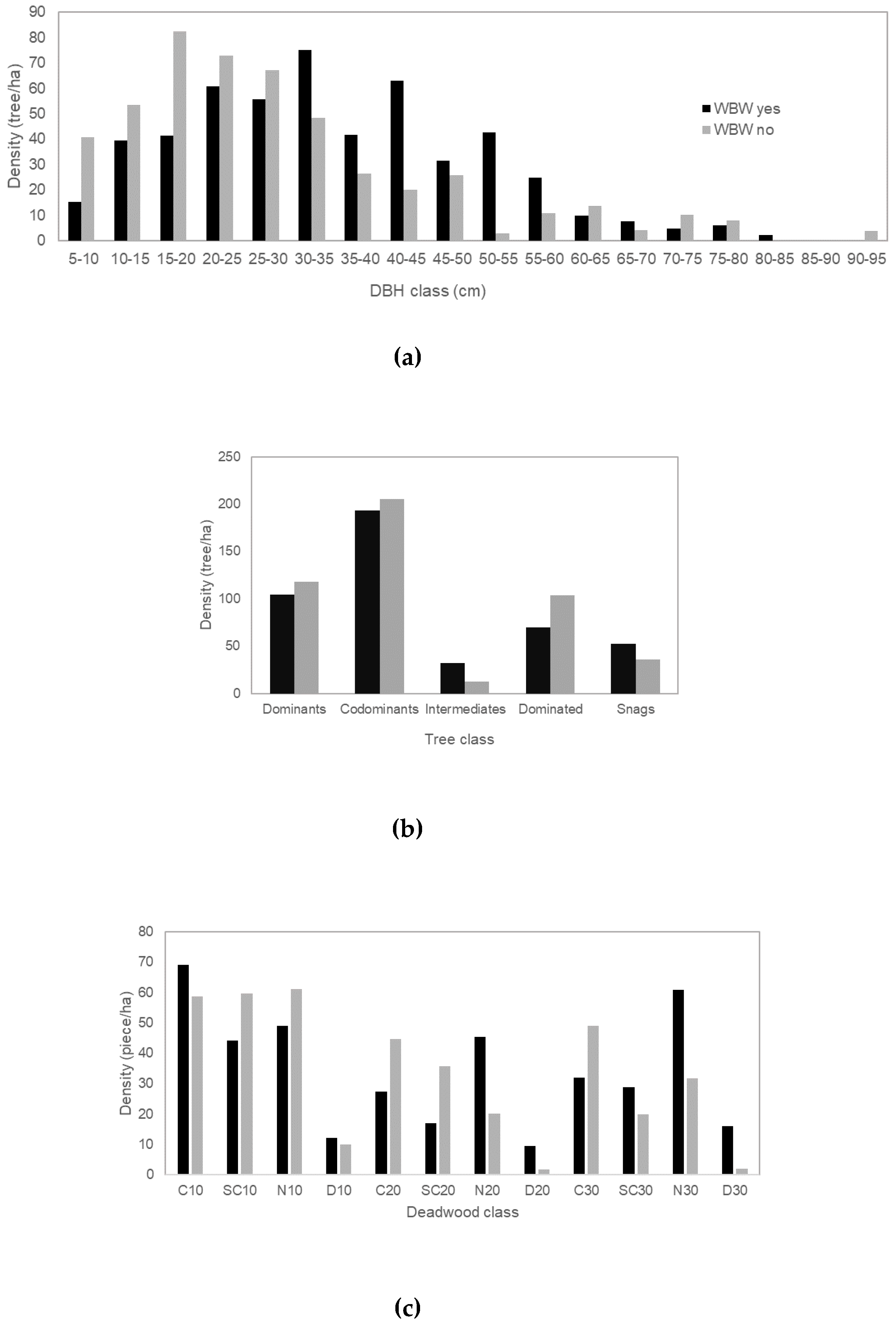
3. Results
4. Discussion
4.1. Key Elements of the WBW Nesting Habitat
4.2. Saproxylic Fungi Community
5. Conclusions
Author Contributions
Funding
Acknowledgments
Conflicts of Interest
Appendix A

| Territory | ||
|---|---|---|
| Quality | WBW Yes | WBW No |
| High | 3P, 4P, 9P,19P, 2T, 3T, 4T | 15P, 16P, 9T |
| Medium | 1P, 2P, 7P, 10P, 20P, 1T, 5T | 5P, 6P, 6T |
| Low | 8P | 11P, 12P, 13P, 14P, 17P, 18P, 7T, 8T, 10T |
Appendix B
| Variables | WBW Yes | WBW No |
|---|---|---|
| (a) Slope (m) | 28 ± 3.19 | 32 ± 3.71 |
| Tree cover (%) | 87 ± 5.44 | 90.5 ± 4.59 |
| DBH (cm) | 35.25 ± 1.84 | 31.7 ± 4.27 |
| DW diversity (Shannon) | 0.77 ± 0.16 | 0.37 ± 0.13 |
| DW volume (m3/ha) | 0.0033 ± 0.0006 | 0.0029 ± 0.0008 |
| Regeneration type 1 (ind./ha) | 6387.24 ± 5028 | 2411.06 ± 1268.14 |
| Regeneration type 2 (ind./ha) | 2007.1 ± 1189.38 | 623.7 ± 623.7 |
| Regeneration type 3 (ind./ha) | 957.18 ± 592.46 | 333.82 ± 261.32 |
| MH diversity (Shannon) | 1.69 ± 0.17 | 1.52 ± 0.17 |
| MHD1 (tree/ha) | 52.98 ± 20.37 | 31.15 ± 12.15 |
| MHD2 (tree/ha) | 142.43 ± 38.66 | 133.66 ± 16.3 |
| MHD3 (tree/ha) | 64.03 ± 15.7 | 45.57 ± 16.07 |
| MHD4 (tree/ha) | 13.58 ± 4.79 | 9.38 ± 6.53 |
| MHD5 (tree/ha) | 139.9 ± 25.21 | 123.65 ± 18.01 |
| MHD6 (tree/ha) | 16.51 ± 8.36 | 15.01 ± 9.2 |
| MHD7 (tree/ha) | 13.58 ± 4.79 | 9.38 ± 6.53 |
| MHD8 (tree/ha) | 22.21 ± 8.88 | 24.2 ± 11.92 |
| MHD9 (tree/ha) | 11.44 ± 6.29 | 0 ± 0 |
| MHD10 (tree/ha) | 119.03 ± 40.16 | 74.85 ± 18.28 |
| MHDtot (tree/ha) | 59.56 ± 11.29 | 46.29 ± 6.75 |
| Dominant (tree/ha) | 104.6 ± 30.35 | 117.7 ± 24.23 |
| Codominant (tree/ha) | 193.01 ± 63.8 | 205.71 ± 20.55 |
| Intermediate (tree/ha) | 32.23 ± 17.59 | 12.45 ± 6.51 |
| Dominated (tree/ha) | 69.98 ± 16.77 | 103.51 ± 43.49 |
| Snag (tree/ha) | 52.15 ± 13.06 | 35.81 ± 15.12 |
| Tree-class diversity (Shannon) | 1.21 ± 0.07 | 1.06 ± 0.07 |
| Tree density (tree/ha) | 468.45 ± 66.38 | 383.98 ± 33.36 |
| Fungi taxa number in sample plots | 6 ± 0.89 | 5.7 ± 0.78 |
| (b) Snag basal area (m2/ha) | 3.48 ± 0.97 | 1.25 ± 0.91 |
| Snag density (snag/ha) | 43.52 ± 10.37 | 19.05 ± 5.6 |
| DW diversity (Simpson) | 0.09 ± 0.01 | 0.11 ± 0.01 |
| Fungi taxa number in transects | 9 ± 0.35 | 7.4 ± 0.87 |
| L10C deadwood-class density (piece/ha) | 66.69 ± 18.47 | 51.87 ± 10.98 |
| L10SC deadwood-class density (piece/ha) | 39.88 ± 7.85 | 52.33 ± 9.95 |
| L10N deadwood-class density (piece/ha) | 44.08 ± 14.93 | 59.86 ± 11.09 |
| L10D deadwood-class density (piece/ha) | 10.69 ± 2.23 | 8.58 ± 5.1 |
| L20C deadwood-class density (piece/ha) | 23.32 ± 6.34 | 37.49 ± 9.44 |
| L20SC deadwood-class density (piece/ha) | 13.08 ± 4.69 | 14.76 ± 4.84 |
| L20N deadwood-class density (piece/ha) | 35.8 ± 5.39 | 17.39 ± 7.71 |
| L20D deadwood-class density (piece/ha) | 3.31 ± 1.63 | 1.6 ± 1.6 |
| L30C deadwood-class density (piece/ha) | 19.74 ± 4.95 | 30.74 ± 11.49 |
| L30SC deadwood-class density (piece/ha) | 7.72 ± 4.75 | 10.67 ± 9.09 |
| L30N deadwood-class density (piece/ha) | 48.49 ± 10.36 | 21.33 ± 19.71 |
| L30D deadwood-class density (piece/ha) | 13.23 ± 5.71 | 0.67 ± 0.67 |
| Z10C deadwood-class density (piece/ha) | 0 ± 0 | 4.8 ± 4.8 |
| Z10SC deadwood-class density (piece/ha) | 0.89 ± 0.89 | 0.67 ± 0.67 |
| Z10N deadwood-class density (piece/ha) | 2.87 ± 1.76 | 1.33 ± 1.33 |
| Z10D deadwood-class density (piece/ha) | 0 ± 0 | 0 ± 0 |
| Z20C deadwood-class density (piece/ha) | 2.81 ± 1.73 | 5.78 ± 2.93 |
| Z20SC deadwood-class density (piece/ha) | 2.96 ± 2.96 | 0.67 ± 0.67 |
| Z20D deadwood-class density (piece/ha) | 2.96 ± 2.96 | 0 ± 0 |
| Z30C deadwood-class density (piece/ha) | 7.82 ± 0.92 | 3.17 ± 2.42 |
| Z30SC deadwood-class density (piece/ha) | 4.7 ± 2.67 | 0.67 ± 0.67 |
| Z30N deadwood-class density (piece/ha) | 9.78 ± 3.59 | 2.67 ± 2.67 |
| Z30D deadwood-class density (piece/ha) | 0 ± 0 | 0 ± 0 |
| T10C deadwood-class density (piece/ha) | 2.5 ± 1.55 | 1.96 ± 1.3 |
| T10SC deadwood-class density (piece/ha) | 3.33 ± 3.33 | 6.76 ± 5.01 |
| T10N deadwood-class density (piece/ha) | 2.06 ± 1.56 | 0 ± 0 |
| T10D deadwood-class density (piece/ha) | 1.48 ± 1.48 | 1.33 ± 1.33 |
| T20C deadwood-class density (piece/ha) | 1.39 ± 1.39 | 1.25 ±1.25 |
| T20SC deadwood-class density (piece/ha) | 0.89 ± 0.89 | 20.28 ± 12.1 |
| T20N deadwood-class density (piece/ha) | 1.11 ± 1.11 | 2.62 ± 1.61 |
| T20D deadwood-class density (piece/ha) | 3.11 ± 2.18 | 0 ± 0 |
| T30C deadwood-class density (piece/ha) | 4.43 ± 1.43 | 15.21 ± 10.34 |
| T30SC deadwood-class density (piece/ha) | 16.48 ± 6.16 | 8.45 ± 4.11 |
| T30N deadwood-class density (piece/ha) | 2.67 ± 2.15 | 7.87 ± 4.91 |
| T30D deadwood-class density (piece/ha) | 2.72 ± 1.71 | 1.33 ± 1.33 |
| C decomposition-state density (piece/ha) | 128.7 ± 21.02 | 152.27 ± 27.18 |
| SC decomposition-state density (piece/ha) | 89.94 ± 17.77 | 115.25 ± 22.42 |
| N decomposition-state density(piece/ha) | 155.32 ± 19.26 | 113.08 ± 34.21 |
| D decomposition-state density (piece/ha) | 37.51 ± 9.13 | 13.51 ± 6.93 |
| E10 diameter deadwood density (piece/ha) | 33.11 ± 9.51 | 37.08 ± 5.28 |
| E20 diameter deadwood density (piece/ha) | 18.01 ± 4.11 | 18.43 ± 3.13 |
| E30 diameter deadwood density (piece/ha) | 25.17 ± 5.5 | 19.35 ± 8.31 |
Appendix C
| Fungi Species | WBW Yes | WBW No |
|---|---|---|
| Hypoxylon fragiforme | +++ | +++ |
| Hypoxylon cohaerens | +++ | +++ |
| Stereum hirsuta | + | + |
| Stereum gausapatum | + | + |
| Stereum insignitum | + | + |
| Stereum sp. | + | - |
| Trametes versicolor | + | + |
| Trametes gibbosa | + | + |
| Trametes ochracea | + | - |
| Exidia glandulosa | + | + |
| Myxarium nucleatum | + | + |
| Eutypella quaternata | + | ++ |
| Bertia moriformis | ++ | ++ |
| Chlorociboria aeruginascens | +++ | ++ |
| Biscogniauxia nummularia | ++ | ++ |
| Diatrype disciformis | ++ | + |
| Nemania serpens | + | - |
| Nemania carbonacea | + | + |
| Ganoderma applanatum | - | + |
| Fomes fomentarius | ++ | - |
| Fomitopsis pinicola | + | + |
| Phellinus igniarius | + | + |
| Loweomyces fractipes | + | + |
| Pleurotus ostreatus | + | + |
| Henningsomyces candidus | + | - |
| Polyporus tuberaster | + | - |
| Pholiota sp. | + | - |
| Entoloma hebes | - | + |
| Polyporus sp. | + | + |
| Phlebia radiata | + | + |
| Nectria cinnabarina | - | + |
| Schizophyllum commune | - | + |
| Lenzites betulina | - | + |
| Dacrymyces stillatus | + | - |
| Crustomyces subabruptus | + | - |
| Junghuhnia lacera | - | + |
| Dentipellis fragilis | + | - |
| Non-identified | - | + |
References
- Virkkala, R.; Alanko, T.; Laine, T.; Tiainen, J. Population contraction of the white-backed woodpecker Dendrocopos leucotos in Finland as a consequence of habitat alteration. Biol. Conserv. 1993, 66, 47–53. [Google Scholar] [CrossRef]
- Winkler, H.; Christie, D.A. Family Picidae (woodpeckers). In Handbook of the Birds of the World; Lynx Edicions: Barcelona, Spain, 2002; Volume 7, pp. 296–555. [Google Scholar]
- Grangé, J.L. Breeding biology of the Lilford Woodpecker Dendrocopos leucotos lilfordi in the Western Pyrenees (SW France). Denisia 36 Zugleich Kataloge des Oberösterreichischen Landesmus. 2016, 164, 99–111. [Google Scholar]
- Grangé, J.L. Le Pic à dos blanc Dendrocopos leucotos lilfordi dans les Pyrénées françaises. Ornithos 2001, 8-1, 8–17. [Google Scholar]
- Garmendia, A.; Cárcamo, S.; Schwendtner, O. Forest management considerations for conservation of black woodpecker Dryocopus martius and white-backed woodpecker Dendrocopos leucotos populations in Quinto Real (Spanish Western Pyrenees). Biodivers. Conserv. 2006, 15, 339–355. [Google Scholar]
- Cárcamo, S. Distribution du Pic de Lilford Dendrocopos leucotos lilfordi à l’ouest des Pyrénées espagnoles. Le Casseur d’os 2016, 16, 96–104. [Google Scholar]
- Brooks, J. Handbook of the birds of Europe, the Middle East and Nord Africa; Oxford University Press: Oxford, UK, 1985; Volume 4. [Google Scholar]
- Global Forest Watch. Available online: https://www.globalforestwatch.org/ (accessed on 13 March 2019).
- Barnard, B.; Garmendia, A.; Schwendtner, O. Caracterización del Hábitat del pico Dorsiblanco (Dendrocopos leucotos) y Propuesta de Gestión en los Hayedos del Monte Mortua (Navarra). Master’s Thesis, Universitat Politècnica de València, Valencia, Spain, 2015. [Google Scholar]
- Shurulinkov, P.; Stoyanov, G.; Komitov, E.; Daskalova, G.; Ralev, A. Contribution to the knowledge on distribution, number and habitat preferences of rare and endangered birds in Western Rhodopes Mts, Southern Bulgaria. Strigiformes and Piciformes. Acta Zool. Bulg. 2012, 64, 43–56. [Google Scholar]
- Domokos, E.; Cristea, V. Effects of managed forests structure on woodpeckers (Picidae) in the Niraj valley (Romania): Woodpecker populations in managed forests. North-West J. Zool. 2013, 10, 110–117. [Google Scholar]
- Jusino, M.A.; Lindner, D.L.; Banik, M.T.; Rose, K.R.; Walters, J.R. Experimental evidence of a symbiosis between red-cockaded woodpeckers and fungi. Proc. R. Soc. B 2016, 283, 20160106. [Google Scholar] [CrossRef]
- Jankowiak, R.; Ciach, M.; Bilański, P.; Linnakoski, R. Diversity of wood-inhabiting fungi in woodpecker nest cavities in southern Poland. Act. Mycol. 2019, 54, 1126. [Google Scholar] [CrossRef]
- Bull, E.L.; Parks, C.G.; Torgersen, T.R. Trees and Logs Important to Wildlife in the Interior Columbia River Basin; U.S. Department of Agriculture; Forest Service Pacific Northwest Research Station; Forest Service; Pacific Northwest Research Station: Corvallis, OR, USA, 1997; p. 55.
- Jackson, J.A.; Jackson, B.J.S. Ecological relationships between fungi and woodpecker cavity sites. Condor 2004, 106, 37–49. [Google Scholar] [CrossRef]
- Kosiński, Z.; Winiecki, A. Nest-site selection and niche partitioning among the Great Spotted Woodpecker Dendrocopos major and Middle Spotted Woodpecker Dendrocopos medius in riverine forest of Centra Europe. Ornis Fennica 2004, 81, 145–156. [Google Scholar]
- Abrego, N.; Salcedo, I. How does fungal diversity change based on woody debris type? A case study in Northern Spain. Ekologija 2011, 57, 109–119. [Google Scholar] [CrossRef] [Green Version]
- Abrego, N.; Salcedo, I. Variety of woody debris as the factor influencing wood-inhabiting fungal richness and assemblages: Is it a question of quantity or quality? For. Ecol. Manag. 2013, 291, 377–385. [Google Scholar] [CrossRef]
- Abrego, N.; Salcedo, I. Response of wood-inhabiting fungal community to fragmentation in a beech forest landscape. Fungal Ecol. 2014, 8, 18–27. [Google Scholar] [CrossRef]
- Roberge, J.M.; Mikusinski, G.; Svensson, S. The white-backed woodpecker: Umbrella species for forest conservation planning? Biodivers. Conserv. 2008, 17, 2479–2494. [Google Scholar] [CrossRef]
- Martikainen, P.; Kaila, L.; Haila, Y. Threatened beetles in white-backed woodpecker habitats. Conserv. Biol. 1998, 2, 293–301. [Google Scholar] [CrossRef]
- Aemet. Esteribar, Eugui. Available online: http://www.aemet.es/es/eltiempo/observacion/ultimosdatos?l=9257X (accessed on 30 July 2019).
- Cárcamo, S. Evolución de las poblaciones de Pito Negro (Drycopus martius) y Pico Dorsiblanco (Dendrocopos luecotos lilfordi) en los montes de Quinto Real (Navarra) y su relación con la gestión forestal. Pirineos 2006, 161, 133–150. [Google Scholar]
- Google Earth. Available online: https://www.google.com/earth/ (accessed on 2 June 2020).
- Commarmot, B. (Ed.) Inventory of the Largest Primeval Beech Forest in Europe: A Swiss-Ukrainian Scientific Adventure; Swiss Federal Inst. for Forest Snow and Landscape Research: Birmensdorf, Switzerland; Ukrainian National Forestry University: L’viv, Ukraine; Carpathian Biosphere Reserve: Rakhiv, Ukraine, 2013. [Google Scholar]
- Magurran, A.E. Measuring Biological Diversity; John Wiley & Sons: Hoboken, NJ, USA, 2013. [Google Scholar]
- R Core Team. R: A Language and Environment for Statistical Computing; R Foundation for Statistical Computing: Vienna, Austria, 2013; Available online: http://www.R-project.org/ (accessed on 11 July 2019).
- Chao, A.; Chiu, C.; Jost, L. Phylogenetic diversity measures based on Hill numbers. Philos. Trans. R. Soc. B 2010, 365, 3599–3609. [Google Scholar] [CrossRef]
- Frenández, C.; Azkona, P. Influence of forest structure on the density and distribution of the White-Backed Woodpecker Dendrocopos leucotos and Black Woodpecker Dryocopus martius in Quinto Real (Spanish western Pyrenees). Bird Study 1996, 43, 305–313. [Google Scholar] [CrossRef] [Green Version]
- Gerdzhikov, G.P.; Georgiev, K.B.; Plachiyski, D.G.; Zlatanov, T.; Shurulinkov, P.S. Habitat Requirements of the White-backed Woodpecker Dendrocopos leucotos lilfordi (Sharpe & Dresser, 1871) (Piciformes: Picidae) in Strandzha Mountain, Bulgaria. Acta Zool. Bulg. 2018, 70, 527–534. [Google Scholar]
- Cárcamo, S.; Elosegi, M.M.; Senosiain, A.; Arizaga, J. Nidotópica y parámetros reproductivos en el pico dorsiblanco Dendrocopos leucotos lilfordi Sharpe & Dresser, 1871 en Navarra. Munibe Cienc. Nat. 2019, 67. [Google Scholar] [CrossRef]
- Bilek, L.; Remes, J.; Zahradnik, D. Managed versus unmanaged. Structure of beech forest stands” Fagus sylvatica L.” after 50 years of development, Central Bohemian. For. Syst. 2011, 20, 122–138. [Google Scholar]
- Vandekerkhove, K.; Vanhellemont, M.; Vrška, T.; Meyer, P.; Tabaku, V.; Thomaes, A.; Leyman, A.; de Keersmaeker, L.; Verheyen, K. Very large trees in a lowland old-growth beech (Fagus sylvatica L.) forest: Density, size, growth and spatial patterns in comparison to reference sites in Europe. For. Ecol. Manag. 2018, 417, 1–17. [Google Scholar] [CrossRef]
- Winter, S.; Brambach, F. Determination of a common forest life cycle assessment method for biodiversity evaluation. For. Ecol. Manag. 2011, 262, 2120–2132. [Google Scholar] [CrossRef]
- Larrieu, L.; Cabanettes, A.; Gonin, P.; Lachat, T.; Paillet, Y.; Winter, S.; Bouget, C.; Deconchat, M. Deadwood and tree microhabitat dynamics in unharvested temperate mountain mixed forests: A life-cycle approach to biodiversity monitoring. For. Ecol. Manag. 2014, 334, 163–173. [Google Scholar] [CrossRef]
- Keren, S.; Diaci, J. Comparing the quantity and structure of deadwood in selection managed and old-growth forests in South-East Europe. Forests 2018, 9, 76. [Google Scholar] [CrossRef] [Green Version]
- Czeszczewik, D. Foraging behaviour of White-backed Woodpeckers Dendrocopos leucotos in a primeval forest (Białowieża National Park, NE Poland): Dependence on habitat resources and season. Acta Ornithol. 2009, 44, 109–118. [Google Scholar] [CrossRef]
- Aulén, G. Ecology and Distribution History of the Whitebacked Woodpecker Dendrocopos leucotos in Sweden. Ph.D. Thesis, Swedish University of Agricultural Sciences, Uppsala, Sweden, 1998. [Google Scholar]
- Hogstad, O.; Stenberg, I. Habitat selection of a viable population of white-backed woodpeckers Dendrocopos leucotos. Fauna Norv. 1994, 17, 75–94. [Google Scholar]
- Czeszczewik, D. Marginal differences between random plots and plots used by foraging White-backed Woodpeckers demonstrates supreme primeval quality of the Białowieża National Park, Poland. Ornis Fenn. 2009, 86, 30–37. [Google Scholar]
- Nordén, B.; Ryberg, M.; Götmark, F.; Olausson, B. Relative importance of coarse and fine woody debris for the diversity of wood-inhabiting fungi in temperate broadleaf forests. Biol. Conserv. 2004, 117, 1–10. [Google Scholar] [CrossRef]
- Brin, A.; Bouget, C.; Brustel, H.; Jactel, H. Diameter of downed woody debris does matter for saproxylic beetle assemblages in temperate oak and pine forests. J. Insect Conserv. 2011, 15, 653–669. [Google Scholar] [CrossRef]
- Aranzadi Zientzia Elkartea. Fitxa Mikologikoa. Available online: http://www.aranzadi.eus/category/micologia?lang=eu (accessed on 3 June 2019).
- Baum, S.; Sieber, T.N.; Schwarze, F.W.; Fink, S. Latent infections of Fomes fomentarius in the xylem of European beech (Fagus sylvatica). Mycol. Prog. 2003, 2, 141–148. [Google Scholar] [CrossRef]
- Song, Z.; Kennedy, P.G.; Liew, F.J.; Schilling, J.S. Fungal endophytes as priority colonizers initiating wood decomposition. Funct. Ecol. 2017, 31, 407–418. [Google Scholar] [CrossRef]
- O’Daniels, S.T.; Kesler, D.C.; Mihail, J.D.; Webb, E.B.; Werner, S.J. Visual cues for woodpeckers: Light reflectance of decayed wood varies by decay fungus. Wilson J. Ornithol. 2018, 130, 200–212. [Google Scholar] [CrossRef]


| Variable | WBW | Non-WBW | Statistic | p-Value |
|---|---|---|---|---|
| (a) Altitude (m) | 897.5 ± 21.87 | 769 ± 15.65 | W = 94 | 0.0009 |
| Tree height (m) | 20.27 ± 0.97 | 14.54 ± 1.04 | t = 4.034 | 0.0008 |
| Tree basal area (m2/ha) | 58.12 ± 5.34 | 42.96 ± 10.59 | W = 82 | 0.0147 |
| Snag basal area (m2/ha) | 3.48 ± 0.97 | 1.25 ± 0.91 | W = 77 | 0.0423 |
| Tree-class diversity (Simpson) | 0.26 ± 0.04 | 0.36 ± 0.03 | t = −2.067 | 0.0553 * |
| (b) Deadwood diversity (Shannon) | 2.59 ± 0.06 | 2.32 ± 0.08 | t = 2.618 | 0.0320 |
| Snag volume (m3/ha) | 6.16 ± 0.64 | 1.19 ± 0.34 | t = 6.878 | 0.0004 |
| Z20N (piece/ha) | 8.46 ± 2.74 | 0 ± 0 | W = 22.5 | 0.0254 |
© 2020 by the authors. Licensee MDPI, Basel, Switzerland. This article is an open access article distributed under the terms and conditions of the Creative Commons Attribution (CC BY) license (http://creativecommons.org/licenses/by/4.0/).
Share and Cite
Urkijo-Letona, A.; Cárcamo, S.; Peña, L.; Fernández de Manuel, B.; Onaindia, M.; Ametzaga-Arregi, I. Key Elements of the White-Backed Woodpecker’s (Dendrocopos leucotos lilfordi) Habitat in Its European South-Western Limits. Forests 2020, 11, 831. https://doi.org/10.3390/f11080831
Urkijo-Letona A, Cárcamo S, Peña L, Fernández de Manuel B, Onaindia M, Ametzaga-Arregi I. Key Elements of the White-Backed Woodpecker’s (Dendrocopos leucotos lilfordi) Habitat in Its European South-Western Limits. Forests. 2020; 11(8):831. https://doi.org/10.3390/f11080831
Chicago/Turabian StyleUrkijo-Letona, Ainhoa, Susana Cárcamo, Lorena Peña, Beatriz Fernández de Manuel, Miren Onaindia, and Ibone Ametzaga-Arregi. 2020. "Key Elements of the White-Backed Woodpecker’s (Dendrocopos leucotos lilfordi) Habitat in Its European South-Western Limits" Forests 11, no. 8: 831. https://doi.org/10.3390/f11080831