A New Approach for Modeling Volume Response from Mid-Rotation Fertilization of Pinus taeda L. Plantations

Abstract

Mid-rotation fertilization presents an opportunity to increase the economic return of plantation forests in the southeastern United States (SEUS). For this reason, the Forest Productivity Cooperative established a series of mid-rotation fertilization trials in Pinus taeda L. plantations across the SEUS between 1984 and 1987. These trials identified site-specific responses to nitrogen (N) and phosphorus (P) fertilizers, resulting in increased stand production for 6–10 years after fertilization. There are successful volume response models that allow users to quantify the gain in stand productivity resulting from fertilization. However, all the current models depend on empirical relationships that are not bounded by biological response, meaning that greater fertilizer additions continue to create more volume gains, regardless of physiological limits. To address this shortcoming, we developed a bounded response model that evaluates relative volume response gain to fertilizer addition. Site index and relative spacing are included as model parameters to help provide realistic estimates. The model is useful for evaluating productivity gain in Pinus taeda stands that are fertilized with N and P in mid-rotation.

1. Introduction

Silvicultural practices are constantly changing in plantation forests [1]. Hence, forest growth and yield systems that are able to predict the effect of different silvicultural practices on stand growth are essential tools needed to guide operational decision-making [2]. Systems with enough flexibility to estimate forest productivity, under a variety of silvicultural practices and management regimes, are available in the literature for common production species [3,4,5].

Soil nutrient availability typically limits forest production [6,7], emphasizing the importance of ameliorating soil nutrient deficiencies in order to enhance forest productivity [8]. To overcome this limitation, the application of N and P for mid-rotation stands has become a regular practice to increase forest productivity [9]. Hence, volume response models for fertilization are essential to describe forest stand dynamics and to guide decision making in mid-rotation stands [10].

There is a wide range of literature with respect to response models that successfully estimate productivity gains in plantation forests through mid-rotation fertilization [11,12,13]. For instance, [14] proposed the evaluation of mid-rotation fertilization gains using two equations added on top of stand dominant height and basal area projections. The authors indicated that these functions included all fertilization effects concerning stand volume gain in Pinus taeda stands and assumed there was no interaction between dominant height and basal area responses. Ref [15] expanded this framework to include separate effects for different N fertilization levels and P, but they still used a set of decoupled response equations. That is, the effect on growth and stand development for a combination of treatments was the sum of the responses for each separate treatment.

Ref [10] included the concepts of Type 1 and Type 2 responses to silvicultural treatment in growth and yield models for Pinus radiata in New Zealand, in which the author advocated that the yield form of the new response model was better compared to the approach of [14]. Ref [16] developed a stand-level volume response model as a function of the leaf area index (LAI), foliar N, growth efficiency, quadratic mean diameter, and age for Pinus taeda plantations. The author highlighted the accuracy of the predictions and that mid-rotation fertilization responses were well accounted by cumulative volume gains after 4 years across a wide environmental gradient in the SEUS. Ref [17] developed volume response models for Pinus silvestris stands in Finland using mixed modeling and reported the sites with the expected higher gain in stand volume.

However, all modeling efforts lack the fundamental biological response where stand growth gains decrease as nutrient additions increase, which is a property that is well studied in agricultural crops [18,19]. It is reasonable to assume that other factors limit stand productivity after nutritional constrains have been ameliorated [20]. Hence, a bounded response model is required to limit productivity gain as a maximum fertilization level is reached. At the same time, complexities in the nonlinearities present in a growth and yield model make an additive response an unreasonable assumption, particularly with interacting nutritional factors.

This study aimed to develop a post mid-rotation fertilization volume response model for Pinus taeda stands across the SEUS that is biologically sound and approaches an asymptotic response to fertilization when accounting for differences in initial stand conditions.

2. Materials and Methods

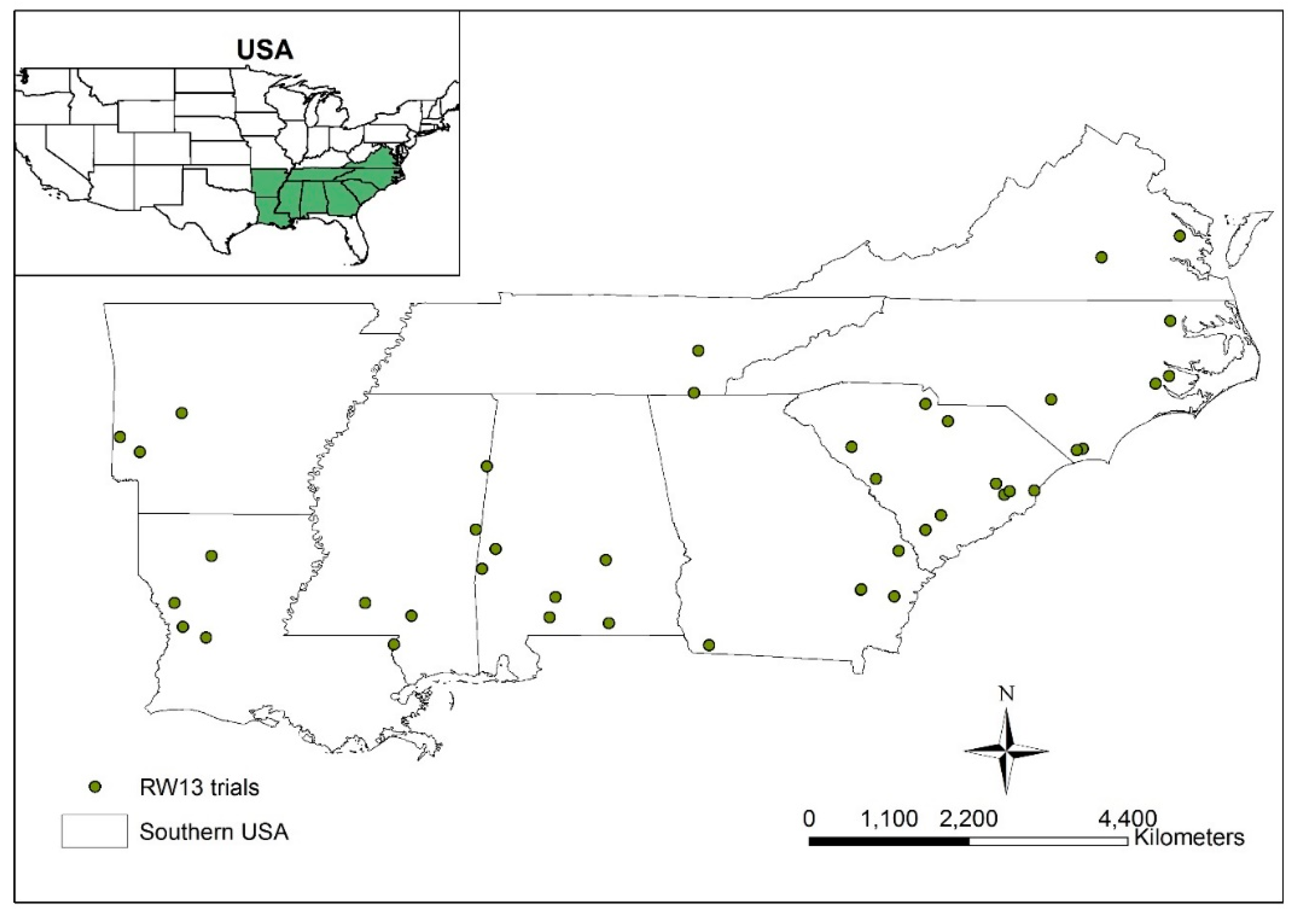
2.1. Study Area and Database Description

The dataset originated from the Regionwide 13 (RW13) trial of the Forest Productivity Cooperative (FPC) Figure 1.

The sites averaged 13 years of age at study establishment. Study sites were established in site prepared, previous loblolly pine plantations (no old field sites) between 1984 and 1987. Sites could have been thinned or unthinned (if thinned at least one year prior to study establishment), had < 1 m² of hardwood basal area as competing vegetation, and no mid-rotation fertilization history (lower coastal plain sites could have received P at establishment). No silvicultural treatments were permitted during the study.

At each site, seven fertilization treatments were applied in a completely randomized block design: control (no fertilization), and a factorial combination of three levels of N (112, 224, 336 kg ha⁻¹) and two levels of P (0 and 28 kg ha⁻¹), as shown in

Table 1. RW13 fertilization treatments.

Treatment	N (kg ha−1)	P (kg ha−1)
1	0	0
2	112	0
3	112	28
4	224	0
5	224	28
6	336	0
7	336	28

. At each site, three replications of each treatment were installed.

Soils ranged in drainage class from well drained to poorly drained and in family particle class size from very fine to sandy. Subsoil texture included clays and sandy clay loams to silt loams.

Table 2. Summary soil chemical characteristics in top 0 to 10 cm and foliar nitrogen before fertilization.

Pretreatment Site Characteristics	Minimum	Average	Maximum
Foliar N (%)	0.87	1.05	1.34
pH	3.78	4.85	7.17
Carbon (%)	0.91	2.03	4.63
Nitrogen (%)	0.02	0.07	0.13
Phosphorus (mg kg−1)	1.04	5.29	17.50

summarizes selected soil and foliar characteristics prior to treatment. Foliage and soil samples were collected in each plot prior to treatments, composited, and analyzed using a CHN analyzer (CE Instruments NC2100 elemental analyzer). Soil phosphorus was determined by Mehlich 3 extraction followed by analysis using inductively coupled plasma-atomic emission spectrophotometry on a Vista-MPX (Varian, Palo Alto, CA, USA). Soil pH was determined with a 1:1 water solution.

All the sites were measured at establishment, as well as 2, 4, 6, and 10 years after fertilization (years since treatment or YST). Site index (base age 25 years) prior to fertilization was estimated for all the sites using a site index equation developed by [15]. Individual tree and stand measurements included diameter at 1.37 m aboveground (DBH, cm), total height (ht in m), dominant height (H in m), and the number of live trees (trees per hectare or TPH).

Sites included in the study represented a wide range in initial stand characteristics, as shown in

Table 3. Summary statistics of the RW13 study at establishment for stand age, number of live trees (TPH), dominant height (H), site index (S), basal area (B), and stand volume (V).

Inventory Variables	Minimum	Average	Maximum
Stand age (years)	9.00	13.40	19.00
TPH	551	1142	2059
H (m)	7.91	12.58	17.51
S (m)	16.64	20.13	24.96
B (m2 ha−1)	11.97	20.83	29.65
V (m3 ha−1)	44.86	120.73	198.05

. Overall, the volume response for N fertilization treatments (compared to the control treatment) varied by P application over time, as shown in Figure 2.

2.2. Model Rationale

2.2.1. Fitting Procedure

Parameters for the response model were found iteratively using an optimization algorithm (Nelder–Mead) that maximized the likelihood of the data (Maximum Likelihood framework):

$$\lambda \left(\theta ,\sigma |x_i,y_i\right)={\displaystyle \sum }_{i=1}^{n}log\left[\frac{1}{\sqrt{2\pi \sigma }}exp\left(\frac{-y_i+f\left(x_i,\theta \right)}{{\sigma }^2}\right)\right]$$

(1)

where $\lambda$ is the log-likelihood; f(·) is a model function with expected parameter $\theta$; y_i is the vector of independent observations for i = 1...n; x_i is the vector of dependent observations for i = 1...n; ${\sigma }^2$ is the expected parameter for the variance; and $\pi$ is a constant.

Least squares is a special case of the Maximum Likelihood (ML), in which the errors are assumed normally distributed, independent, and with constant variance. One of the main advantages of using ML as the fitting procedure is related to its flexibility in allowing for more complex model specifications [4]. The possibility of explicitly modeling the variance (${\sigma }^2$) is needed to further explore the inference around fertilization response and to directly solve for uneven variance along the response period. We used optimization methods to iteratively find parameters to maximize the likelihood (minimize the log-likelihood) using the “optimx” package in R [21].

2.2.2. Data Standardization

Conventionally, treatment response has been calculated as the difference in the target variable for the treated plot minus the control [14]. For volume, the response would be the following:

$$v_{xt}=V_{xt}-V_{1t}$$

(2)

where $v_{xt}$ is the volume response in m³ ha⁻¹ of treatment x at t years since the treatment was established; $V_{xt}$ is the stand level volume in m³ ha⁻¹ of treatment x at t years since the treatment was established; and $V_{1t}$ is the stand level volume in m³ ha⁻¹ of the control treatment at t years since the fertilizer was applied in the other treatments.

The approach works well for experiments followed from establishment, where a carry-over effect in plant reserves might be negligible. However, for treatments applied in established stands at mid-rotation, it is unlikely to have the same starting volume between the control and the fertilization treatments. Stands with different initial sizes are likely to have different amounts of leaf area, and their responses will be correlated to the initial size, potentially obscuring the response of interest. Hence, prior to any evaluation, the dataset was standardized as a relative response with respect to each initial value:

$$r{V}_{xt}=\frac{V_{xt}-V_{x1}}{V_{x1}}$$

(3)

where rV is the relative volume of treatment x at t years since the treatment was established; ${\mathrm{V}}_{\mathrm{x}1}$ is the stand-level volume of treatment x at the time when the treatment was established (t = 0); and other variables are previously defined.

After calculating the relative volume increase for each treatment (rV), the relative volume response is calculated as the difference with respect to the control treatment:

$$r{v}_{xt}=r{V}_{xt}-r{V}_{1t}$$

(4)

where r$v_{xt}$ is the relative volume response of treatment x at t years since the treatment was established; $r{V}_{xt}$ is the stand-level relative volume of treatment x at t years since the treatment was established; and $r{V}_{1t}$ is the stand-level relative volume of control treatment at t years since the fertilizer was applied in the other treatments.

2.2.3. Model Development

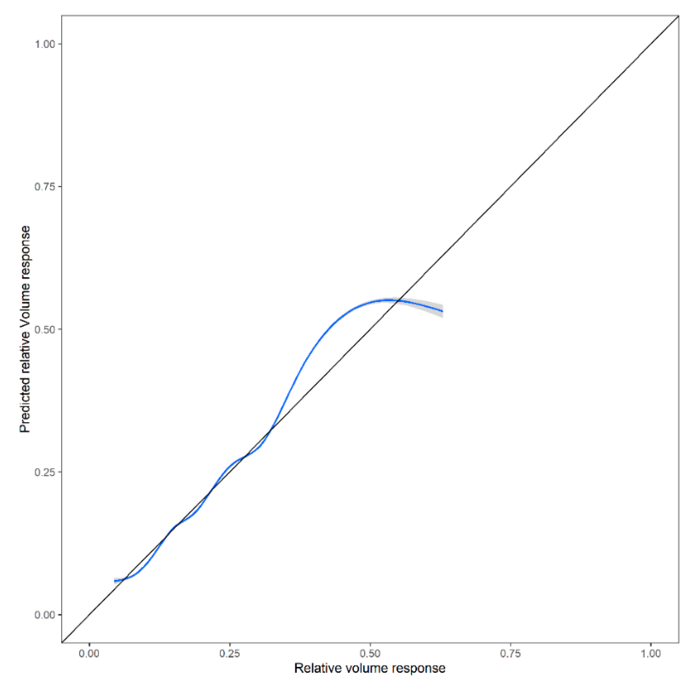
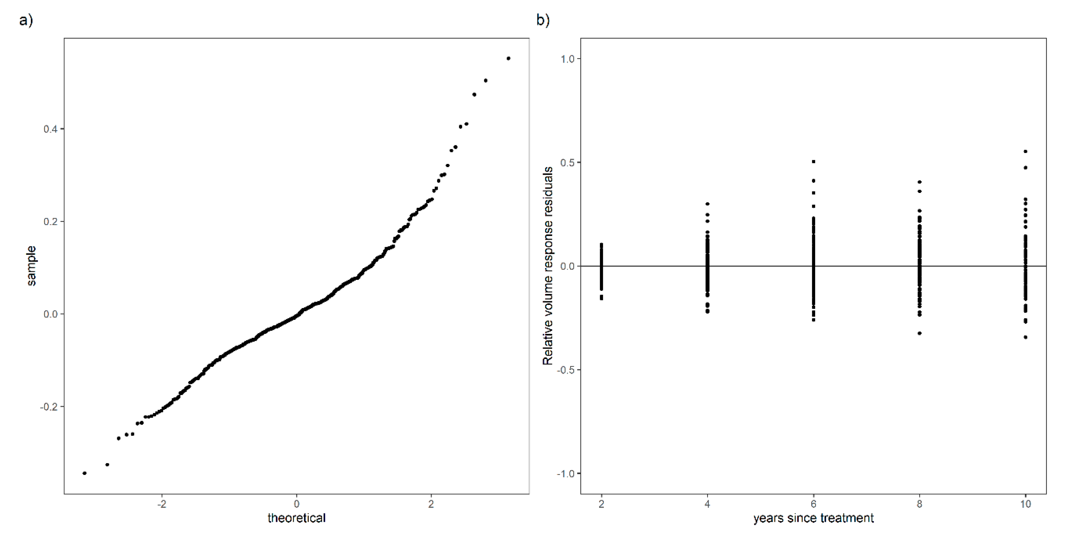
In crop modeling, the Mitscherlich equation is typically applied for quantifying yield response for different fertilization levels:

$$r{v}_x=a\left(1-exp\left(-b{N}_x\right)\right)$$

(5)

where $r{v}_x$ is the relative volume response of treatment x; N is the level of nitrogen in kg ha⁻¹ applied to treatment x; a is the maximum yield at high levels of N; and b is the nutrient response coefficient.

The use of Equation (5) in crop modeling implies that there is a maximum yield (volume response) after a certain level of N applied, as shown in Figure 3.

However, in forest growth modeling, we typically model $r{v}_x$ over time (t):

$$r{v}_{xt}=a\left(1-exp\left(-bt\right)\right)$$

(6)

where $r{v}_{xt}$ is the relative volume response of treatment x at t years since the treatment was established; a is the maximum yield at high t; and b is the time (years, t) response coefficient.

It is assumed through Equation (6) that $r{v}_{xt}$ increases over time until reaching a maximum response (asymptote), regardless of the different levels of N and P applied in the mid-rotation stands, as shown in Figure 4.

Let’s consider the decomposition of the a parameter of Equation (6) as a function of the different levels of N and the presence or absence of P:

$$a=a_0{}^P\left(1-exp\left(-a_{1}N\right)\right)$$

(7)

where P is applied (P = 1) or not (P = 0); all other variables are previously defined.

The asymptote is now constrained by different levels of N and P, which means that the model asymptote changes for different levels of N and their interaction with the application of P is shown in Figure 5.

Hence, the proposed response model is now expressed as:

$$r{v}_{xt}=a_0{}^{P_x}\left(1-exp\left(-a_1{N}_x\right)\right)\left(1-exp\left(-bt\right)\right)$$

(8)

where $r{v}_{xt}$ is the relative volume response of treatment x at t years since the treatment was established; N is level of nitrogen in kg ha⁻¹ applied in treatment x; P is a binary variable indicating the application of phosphorus in treatment x; and the other variables are previously defined.

Equation (8) still displays some shortcomings. The relative volume response is typically higher at sites with lower quality; however, site quality is not represented in the equation. In our dataset, large differences in the initial stand density exist ranging from 551 to 2059 trees ha⁻¹, as shown in Table 3, which are not represented in the equation.

To overcome the lack of site quality information in the model, the site index prior to any fertilization treatment could be incorporated in the model:

$$r{v}_{xt}=a_0{}^{P_x}{\mathrm{S}}^{a_1}\left(1-exp\left(-a_2{N}_x\right)\right)\left(1-exp\left(-bt\right)\right)$$

(9)

where S is the estimated site index in m of each site estimated from the site index equation developed by [15] at the base age of 25 years; other variables are previously defined.

The crown ratio is a variable well correlated with canopy size (commonly assessed as the leaf area index) and gives both a measure of the photosynthetic capacity of a tree or stand density. This variable is conventionally used to provide a measure of tree growing space as well as its competition for nutrients, water, and light. It is worth mentioning that while the leaf area index and crown ratio measurements are not easily available in most forest inventories, [22] found that the crown ratio is accurately predicted by relative spacing (Hart–Becking index). Hence, we may assume that the relative spacing should be monotonically related to the leaf area index, which is a variable that is previously reported to be directly related with the response level [16]. We included relative spacing in the model slope:

$$r{v}_{xt}=a_0{}^{P_x}{\mathrm{S}}^{a_1}\left(1-exp\left(-a_2{N}_x\right)\right)\left(1-exp\left(-\left(b_0+b_{1}RS\right)t\right)\right)$$

(10)

where RS is the relative spacing–$RS=\frac{\sqrt{\frac{10000}{\mathrm{TPH}}}}{\mathrm{H}}$ and H is the dominant height in m; all the other variables were previously defined.

Typically, the linearity of the model errors, independence, and normality of error distribution are assumed [4], although this is rarely the case. We modeled variance using the equation:

$$\sigma ={\beta }_1{\widehat{rv}}_{xt}{}^{{\beta }_2}$$

(11)

where $\beta s$ are the coefficients to be estimated; all the other variables were previously defined. This function enables proper inferences and model extrapolation. This variance function allows the regression assumptions to be met for these data [4]. Variance modeling was completed using a generalized nonlinear regression approach.

2.3. Validation

Ref [23] suggested that the simulation techniques displayed the same power for modeling accuracy evaluation as data splitting. In this study, we used 1000 random samples with repetition generated from the non-parametric bootstrapping technique to evaluate modeling accuracy. This technique was employed by [5], who indicated that it worked well, particularly with extreme cases.

Statistical indices bias (T), mean absolute error (MAE), root mean square error (RMSE), model efficiency (EF), and graphical analyses using the R package ggplot2 [24] were used to evaluate the model.

$$T=\frac{1}{n}{\displaystyle \sum }_{i=1}^n\left(O-Pr\right)$$

(12)

$$MAE=\frac{1}{n}{\displaystyle \sum }_{i=1}^n\left|O-Pr\right|$$

(13)

$$RMSE=\sqrt{\frac{{\sum }_{i=1}^n{\left(Pr-O\right)}^2}{n}}$$

(14)

$$EF=1-\frac{{\sum }_{i=1}^n{\left(O-Pr\right)}^2}{{\sum }_{i=1}^n{\left(O-\overline{O}\right)}^2}$$

(15)

where $Pr$ is the predicted values; $O$ is the observed values; $\overline{O}$ is the mean of the observed values; and $n$ is the number of observations.

3. Results

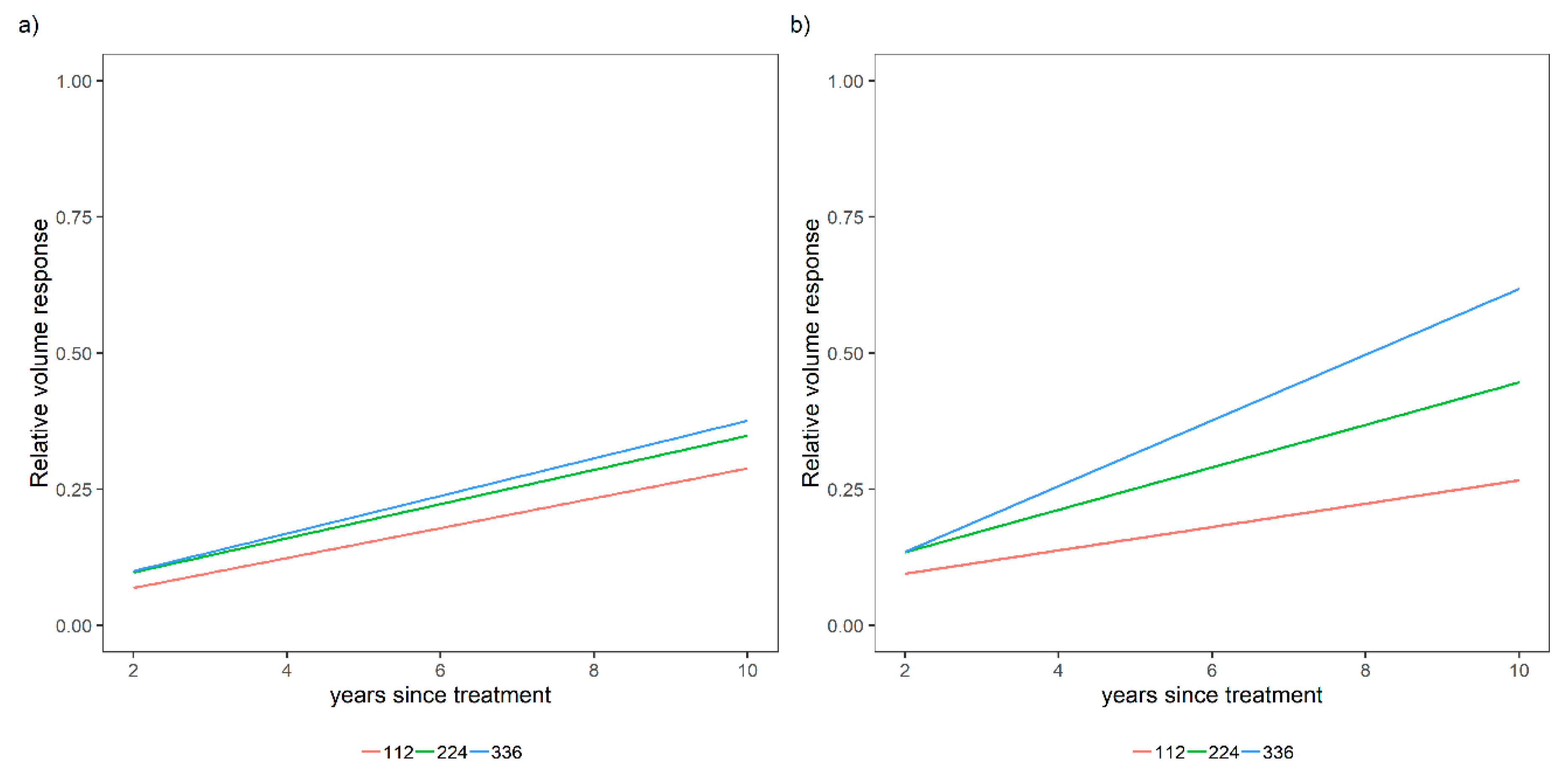
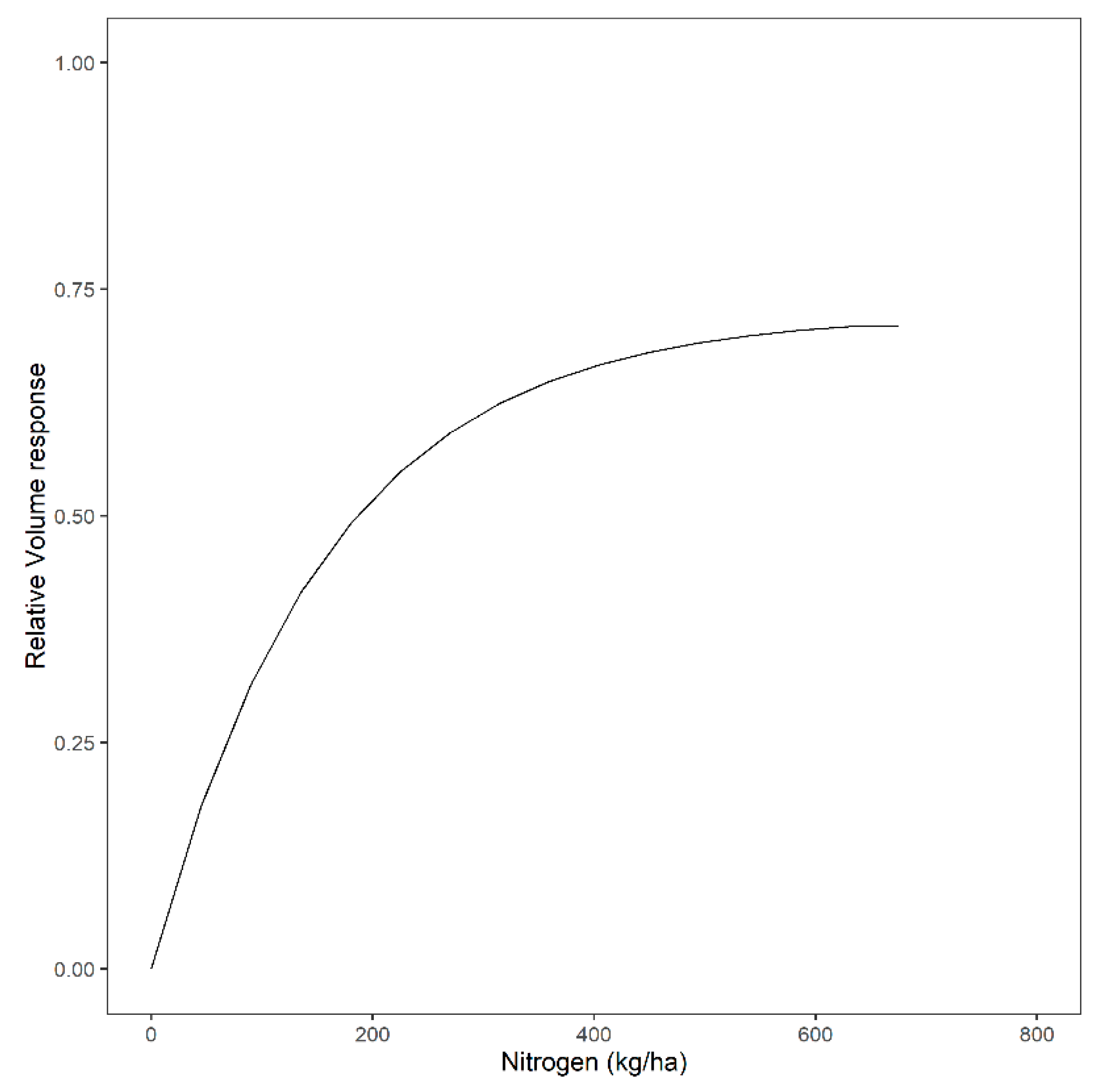
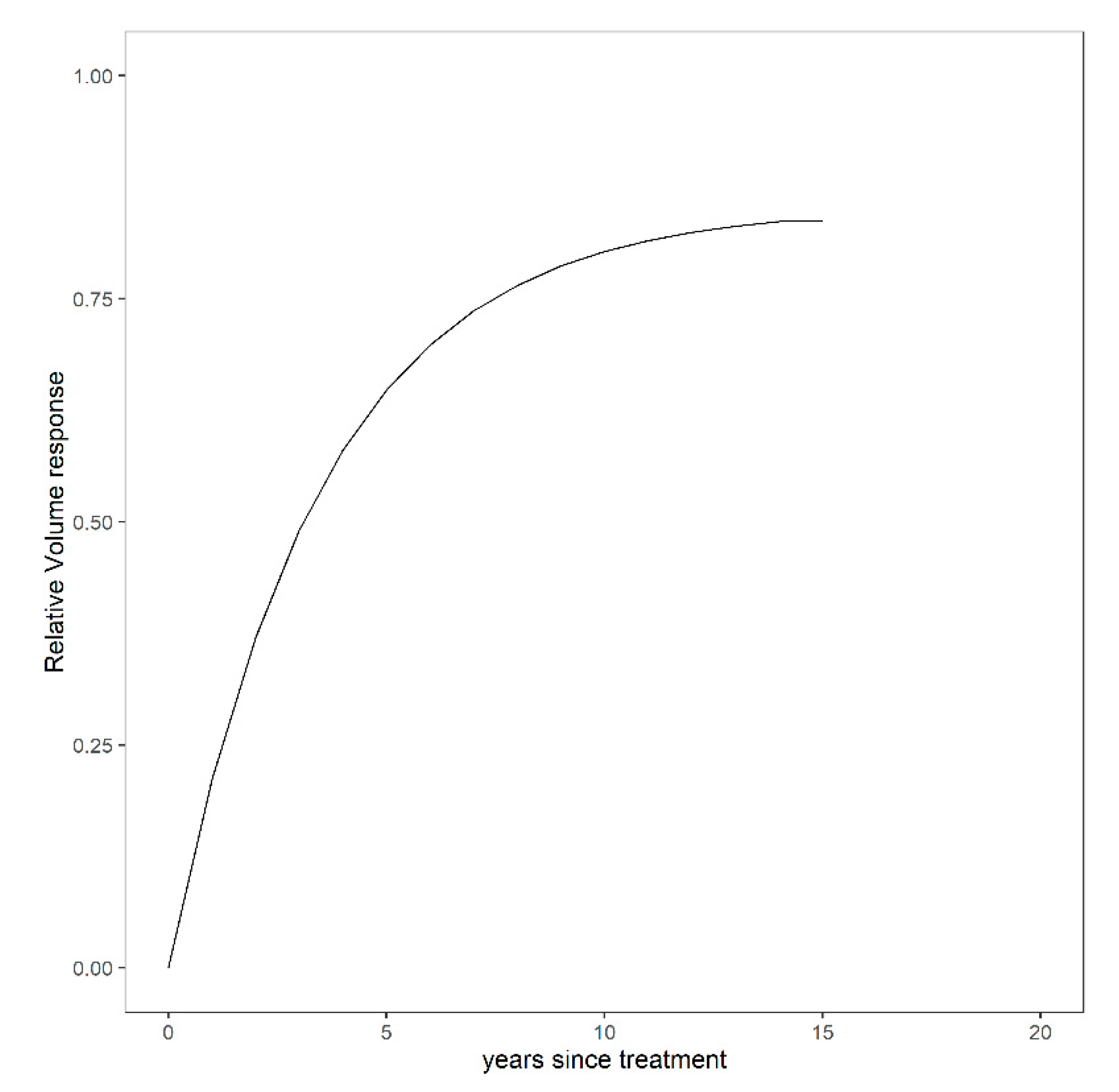
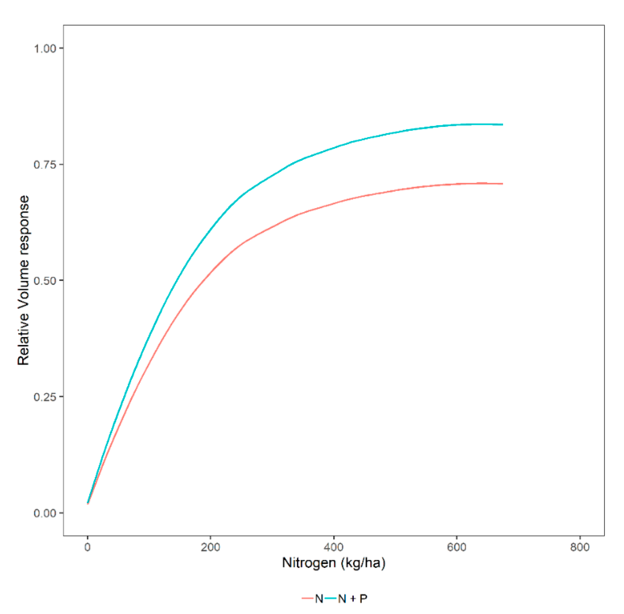
3.1. Overall Relative Volume Response to Different Fertilization Levels

The fitted relative volume response equation and the variance function are

$${\widehat{rv}}_{xt}={1.1878}^P{\mathrm{S}}^{-0.1040}\left(1-exp\left(-0.0079N\right)\right)\left(1-exp\left(-\left(-0.0387+0.4883RS\right)t\right)\right)$$

(16)

$$\widehat{\sigma }=0.4299{\widehat{rv}}_{xt}{}^{0.9671}$$

(17)

where all variables are previously defined.

All the coefficients are significant at alpha = 0.05 and display proper signs. The fitted Equation (16) implies that the stand-level relative volume response increases with higher levels of N and the relative volume response is higher when N and P are applied together. Lower site qualities, represented here by the site index, also display higher relative volume responses for any fertilization practice compared to sites with higher quality. The relative response increases over time for any treatment, and the relative response increases for stands with higher RS, which means that more growing space (lower competition for nutrients x water x light) is available for the trees.

The statistical indices T = 0.006, MAE = 0.07, RMSE = 0.11, and EF = 0.60 indicated an acceptable level of accuracy for the estimates provided by Equation (16). The observed and estimated stand-level relative volume response were well correlated, as shown in Figure 6, but there is still some random variation that the model was not able to explain.

Finally, a variance function (Equation (17)) indicated that the error assumptions were not violated, as shown in Figure 7.

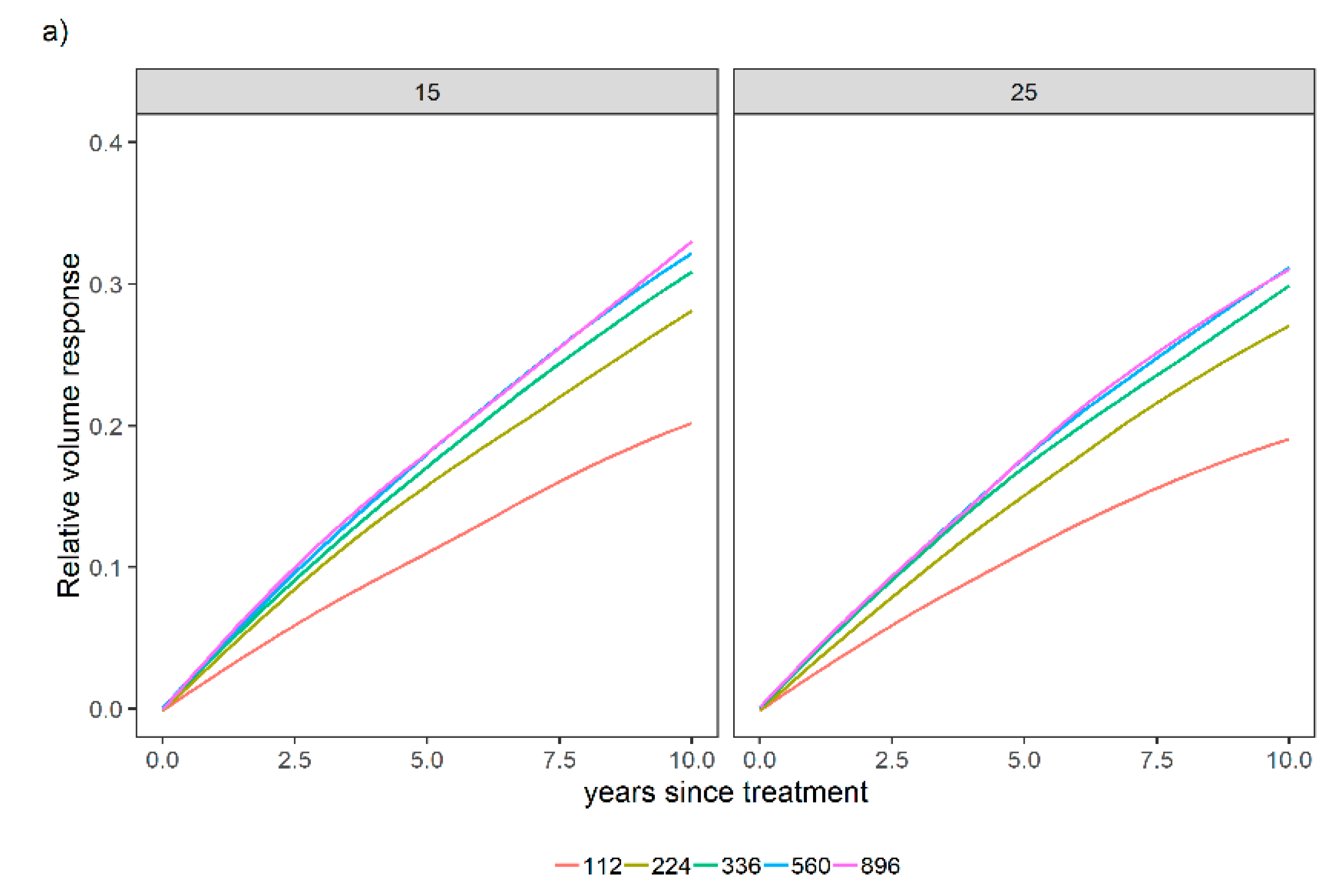
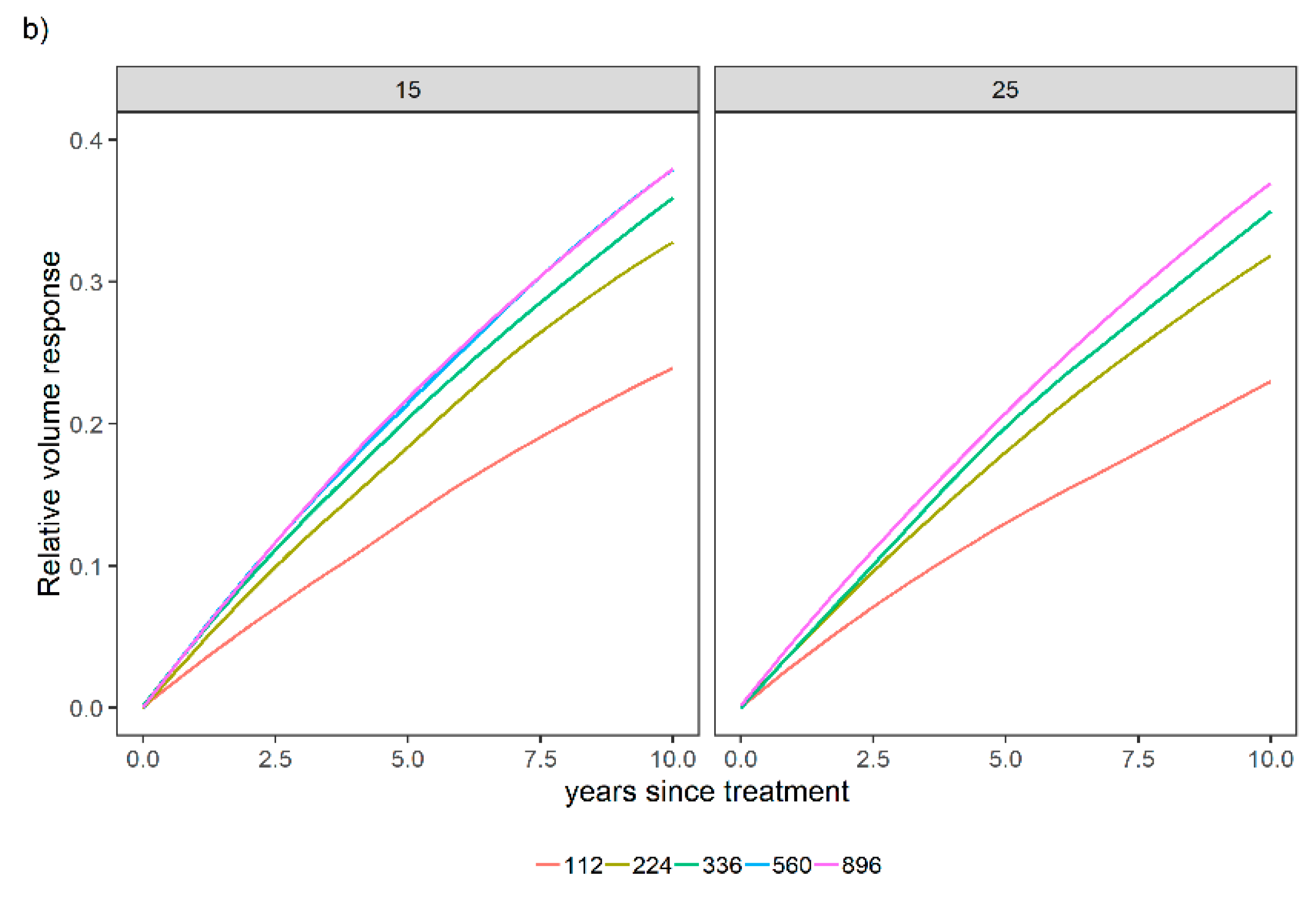
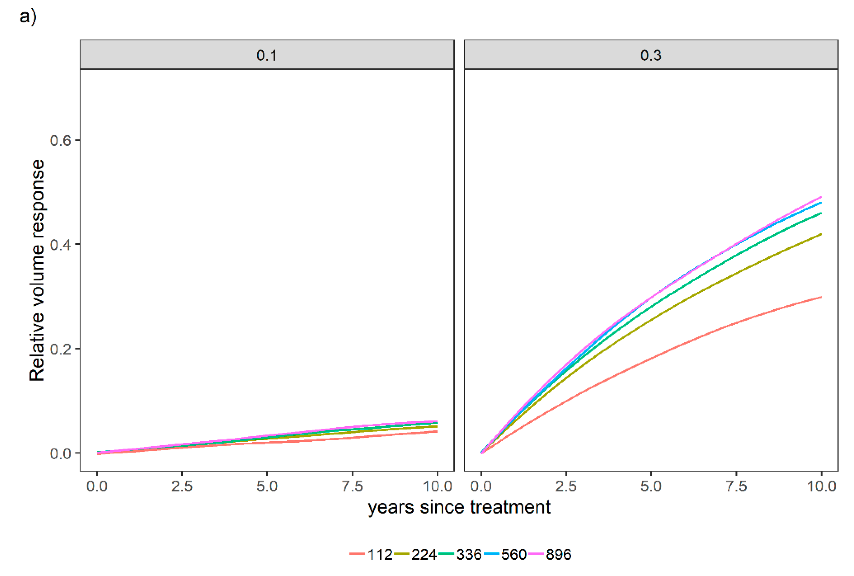
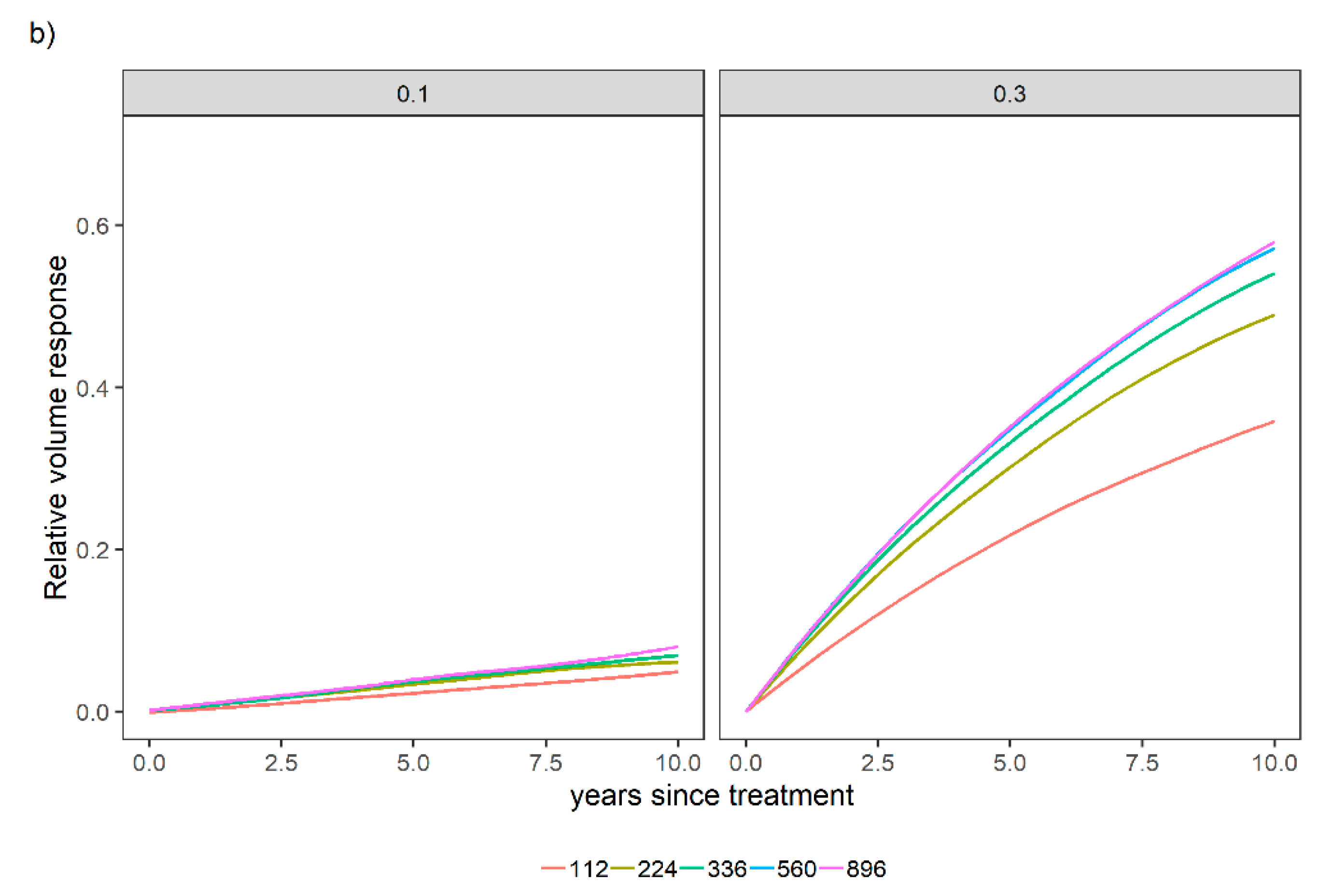
3.2. Sensitivity Analysis for a Variety of Relative Spacing and Site Index Scenarios over a Variety of N and P Levels

Since the model fit well and the underlying assumptions were not violated, Equation (16) can be used with some confidence for making inferences. Thus, Equation (16) was tested for a variety of site index (S) values (Figure 8) and relative spacing (RS) (Figure 9) scenarios for different levels of N (112, 224, 336, 560, and 896 kg ha⁻¹) and P (0 and 28 kg ha⁻¹).

Ref [22] stated a relative spacing bounded between 0.2 and 0.3 as desired in loblolly pine stands. It is worth mentioning at a high level of stocking RS = 0.1 in Figure 9, stands do appear to slightly react to the fertilization treatments, which is due to the limited tree growing space, and this finding agrees with the model hypothesis.

Equation (16) is bounded, which means that the productivity gain of a given site increases with fertilization practices, but there is a limit associated with the fertilization level. These N applications were tested to provide an overview of how the model is bounded, although it is worth mentioning that some of the N applications in Figure 8 and Figure 9 far exceed what was applied in the experiment. Finally, the sensitivity analysis supported the biological soundness of the model approach.

4. Discussion

We introduced a new relative volume response model in this paper to address mid-rotation fertilization gains in Pinus taeda stands across the SEUS. Relative volume response increases with increasing fertilization levels, but there is a maximum relative volume response after a certain fertilization level. The model produced a biologically sound response curve.

The modeling approach developed in this study provided consistent estimates. Ref [25] discussed how important it is to have models with accurate information, because this information is critical for operational decision-making. Additionally, [2,14] demonstrated how useful response model estimates are as an effective tool to address silvicultural questions for a range of site conditions and fertilization levels, especially for mid-rotation Pinus taeda L. stands in southeastern USA (SEUS). These stands are known to be limited by nitrogen (N) and phosphorus (P) availability [26,27]. Hence, the application of N and P at this stage of stand development has become a regular practice to increase forest productivity [9].

Budgetary constraints in the forestry sector indicate how important it is to select the best fertilization regime for a given stand [7,19]. Dramatic growth gains can be obtained with the use of a proper fertilization regime. Consequently, it is essential to have the best analytical tool to allow the decision maker to choose a fertilization regime that maximizes forest growth and profitability [28]. The response model developed in this study will be useful for evaluating the potential productivity gain for Pinus taeda stands that are fertilized with N and P at mid-rotation, because its predictions are accurate and biologically sound. The model structure is also recommended to be applied to commercial plantations with other tree species, since its properties ensure biologically sound estimates.

Our modeling approach examined the mean effect of fertilization response in stands with a large variation in initial stand density and different site qualities. Some random variation could not be explained by our modeling approach in this study, as previously highlighted. We recommend that future studies include LAI in volume response modeling. LAI combined with RS and site index provide extra information to characterize site conditions and especially stand health. For example, in stands with the same RS and site index, but with different relative volume response for the same level of applied N and P, the difference could be explained by including LAI in the analysis, as demonstrated by [4]. LAI is an important variable that relates directly to the ability of a given stand to photosynthesize [1]. Sites with same site index, LAI and RS respond differently based on soils [19] and limitations other than N and P may exist, and these factors should also be examined in future studies.

5. Conclusions

We successfully developed a relative volume response model to predict productivity gains due to mid-rotation fertilization in Pinus taeda stands across the SEUS. The model will help select the appropriate site-specific fertilizer level to apply in a given Pinus taeda stand. The model produces biologically sound output for a variety of relative spacing and site index scenarios. This information will help forest managers maximize forest growth and profitability.

References

1. Stape, J.-L.; Binkley, D.; Ryan, M.G.; Fonseca, S.; Loos, R.A.; Takahashi, E.N.; Silva, C.R.; Silva, S.R.; Hakamada, R.E.; Ferreira, J.M.D.A.; et al. The Brazil Eucalyptus Potential Productivity Project: Influence of water, nutrients and stand uniformity on wood production. For. Ecol. Manag. 2010, 259, 1684–1694. [Google Scholar] [CrossRef]
2. Gyawali, N.; Burkhart, H.E. General response functions to silvicultural treatments in loblolly pine platations. Can. J. For. Res. 2015, 45, 252–265. [Google Scholar] [CrossRef]
3. McTague, J.P.; O’Loughlin, D.; Roise, J.P.; Robison, D.J.; Kellison, R.C. The SOHARC Model System for Growth and Yield of Southern Hardwoods. South. J. Appl. For. 2008, 32, 173–183. [Google Scholar] [CrossRef] [Green Version]
4. Montes, C. A Resource Driven Growth and Yield Model for Loblolly Pine Plantations. Ph.D. Thesis, North Carolina State University, Raleigh, NC, USA, 2012. [Google Scholar]
5. Scolforo, H.F.; McTague, J.P.; Burkhart, H.; Roise, J.; Campoe, O.; Stape, J.L. Eucalyptus growth and yield system: Linking individual-tree and stand-level growth models in clonal Eucalypt plantations in Brazil. For. Ecol. Manag. 2019, 432, 1–16. [Google Scholar] [CrossRef]
6. Allen, H.; Dougherty, P.; Campbell, R. Manipulation of water and nutrients—Practice and opportunity in Southern U.S. pine forests. For. Ecol. Manag. 1990, 30, 437–453. [Google Scholar] [CrossRef]
7. Ramírez, A.M.; Ra, R.; Montes, C.; Hl, A.; Tr, F.; Sanfuentes, E.; Alzate, M.R. Mid-rotation response to fertilizer by Pinus radiata D. Don at three contrasting sites. J. For. Sci. 2016, 62, 153–162. [Google Scholar] [CrossRef] [Green Version]
8. Fox, T.R.; Allen, H.L.; Albaugh, T.J.; Rubilar, R.; Carlson, C.A. Tree Nutrition and Forest Fertilization of Pine Plantations in the Southern United States. South. J. Appl. For. 2007, 31, 5–11. [Google Scholar] [CrossRef] [Green Version]
9. Albaugh, T.J.; Allen, H.L.; Fox, T.R. Historical Patterns of Forest Fertilization in the Southeastern United States from 1969 to 2004. South. J. Appl. For. 2007, 31, 129–137. [Google Scholar] [CrossRef] [Green Version]
10. Snowdon, P. Modeling Type 1 and Type 2 growth responses in plantations after application of fertilizer or other silvicultural treatments. For. Ecol. Manag. 2002, 163, 229–244. [Google Scholar] [CrossRef]
11. Woollons, R.C.; Whyte, A.G.D.; Mead, D.J. Long-term growth responses in Pinus Radiata fertilizer experiments. N. Z. J. For. Sci. 1988, 18, 199–209. [Google Scholar]
12. McInnis, L.M.; Oswald, B.P.; Williams, H.M.; Farrish, K.W.; Unger, D.R. Growth response of Pinus taeda L. to herbicide, prescribed fire, and fertilizer. For. Ecol. Manag. 2004, 199, 231–242. [Google Scholar] [CrossRef]
13. Carlson, C.A.; Fox, T.R.; Allen, H.L.; Albaugh, T.J. Modeling mid-rotation fertilizer responses using the age-shift approach. For. Ecol. Manag. 2008, 256, 256–262. [Google Scholar] [CrossRef]
14. Pienaar, L.; Rheney, J.W. Modeling stand level growth and yield response to silvicultural treatments. For. Sci. 1995, 41, 629–638. [Google Scholar]
15. Amateis, R.; Burkhart, H.; Allen, H.L.; Montes, C. FASTLOB: Fertilized and Selectively Thinned Loblolly Pine Plantations (a Stand-Level Growth and Yield Model for Fertilized and Thinned Loblolly Pine Plantations). In Loblolly Pine Growth and Yield Cooperative; VPISU: Blacksburg, VA, USA, 2001. [Google Scholar]
16. Rojas, J. Factors influencing responses of loblolly pine stands to fertilization. Ph.D. Thesis, North Carolina State University, Raleigh, NC, USA, 2005. [Google Scholar]
17. Hökkä, H.; Repola, J.; Moilanen, M. Modelling volume growth response of young Scots pine (Pinus sylvestris) stands to N, P, and K fertilization in drained peatland sites in Finland. Can. J. For. Res. 2012, 42, 1359–1370. [Google Scholar] [CrossRef]
18. Ingestad, T. Relative addition rate and external concentration; Driving variables used in plant nutrition research. Plant. Cell Environ. 1982, 5, 443–453. [Google Scholar] [CrossRef]
19. Albaugh, T.J.; Fox, T.R.; Allen, H.L.; Rubilar, R. Juvenile Southern Pine Response to Fertilization Is Influenced by Soil Drainage and Texture. Forests 2015, 6, 2799–2819. [Google Scholar] [CrossRef] [Green Version]
20. Mason, E.G.; Milne, P.G. Effects of weed control, fertilization, and soil cultivation on the growth of Pinus radiata at midrotation in Canterbury, New Zealand. Can. J. For. Res. 1999, 29, 985–992. [Google Scholar] [CrossRef]
21. R Core Development Team. R: A Language and Environment for Statistical Computing; R Foundation for Statistical Computing: Vienna, Austria, 2015; Available online: http://www.R-project.org (accessed on 3 May 2019).
22. Zhao, D.; Kane, M.; Borders, B.E. The Crown Ratio and Relative Spacing Relationships for Loblolly Pine Plantation Stands; PMRC Technical Report: Athens, GA, USA, 2009; p. 24. [Google Scholar]
23. Kozak, A.; Kozak, R. Does cross validation provide additional information in the evaluation of regression models? Can. J. For. Res. 2003, 33, 976–987. [Google Scholar] [CrossRef]
24. Wickham, H. Ggplot2: Elegant Graphics for Data Analysis; Springer: New York, NY, USA, 2009; p. 211. [Google Scholar]
25. Miehle, P.; Battaglia, M.; Sands, P.J.; Forrester, D.I.; Feikema, P.M.; Livesley, S.; Morris, J.D.; Arndt, S. A comparison of four process-based models and a statistical regression model to predict growth of Eucalyptus globulus plantations. Ecol. Model. 2009, 220, 734–746. [Google Scholar] [CrossRef]
26. Haines, L.W.; Haines, S.G.; Allen, V.H., Jr. Fertilizing established loblolly pine stands. In Proc. 6th S. Forest Soils Workshop; US Forest: Charleston, SC, USA, 1976; pp. 56–67. [Google Scholar]
27. King, J.S.; Albaugh, T.J.; Allen, H.L.; Buford, M.; Strain, B.R.; Dougherty, P. Below-ground carbon input to soil is controlled by nutrient availability and fine root dynamics in loblolly pine. New Phytol. 2002, 154, 389–398. [Google Scholar] [CrossRef] [Green Version]
28. Fox, T.R. Sustained productivity in intensively managed forest plantations. For. Ecol. Manag. 2000, 138, 187–202. [Google Scholar] [CrossRef]
Figure 1. Distribution of Regionwide 13 (RW13) sites in the southeastern United States (SEUS).
Forests 11 00646 g001
Figure 2. Relative volume response for the N treatments (112, 224, and 336 kg ha−1 elemental N) compared to the control treatment over time for treatments where P was not applied (a) and where 28 kg ha−1 of elemental P was applied (b). These data represent average volume response in SEUS.
Forests 11 00646 g002
Figure 3. Hypothetical relative volume response for different levels of nitrogen (kg ha−1).
Forests 11 00646 g003
Figure 4. Hypothetical relative volume response for any treatment over time (years since the treatments were established).
Forests 11 00646 g004
Figure 5. Hypothetical relative volume response for different levels of nitrogen (kg ha−1) and the interaction with phosphorus, assuming P-limitation exists.
Forests 11 00646 g005
Figure 6. Performance of Equation (16), smooth line of observed stand-level relative volume responses vs. estimated (predicted) stand-level relative volume responses. The validation dataset originated from 1000 random samples generated through the non-parametric bootstrapping technique.
Forests 11 00646 g006
Figure 7. Quantile-quantile plot showing the normality of the residuals (a); Residuals over time (b) do not display a trend.
Forests 11 00646 g007
Figure 8. Relative stand-level volume response for two initial site index scenarios [15 m and 25 m] across different levels of N (112, 224, 336, 560, and 896 kg ha−1) over time (years since treatment was established) when P was not applied (a) or when 28 kg ha−1 of P was applied (b). Relative spacing was held constant (RS = 0.20).
Forests 11 00646 g008aForests 11 00646 g008b
Figure 9. Relative stand-level volume response for two relative spacing scenarios [0.1 and 0.3] across different levels of N (112, 224, 336, 560, and 896 kg ha−1) over time (years since treatment was established) when P was not applied (a) or when 28 kg ha−1 of P was applied (b). Site index was held constant (S = 20 m).
Forests 11 00646 g009aForests 11 00646 g009b