Estimating Coarse Woody Debris Volume Using Image Analysis and Multispectral LiDAR

Abstract

Coarse woody debris (CWD, parts of dead trees) is an important factor in forest management, given its roles in promoting local biodiversity and unique microhabitats, as well as providing carbon storage and fire fuel. However, parties interested in monitoring CWD abundance lack accurate methods to measure CWD accurately and extensively. Here, we demonstrate a novel strategy for mapping CWD volume (m³) across a 4300-hectare study area in the boreal forest of Alberta, Canada using optical imagery and an infra-canopy vegetation-index layer derived from multispectral aerial LiDAR. Our models predicted CWD volume with a coefficient of determination (R2) value of 0.62 compared to field data, and a root-mean square error (RMSE) of 0.224 m³/100 m². Models using multispectral LiDAR data in addition to image-analysis data performed with up to 12% lower RMSE than models using exclusively image-analysis layers. Site managers and researchers requiring reliable and comprehensive maps of CWD volume may benefit from the presented workflow, which aims to streamline the process of CWD measurement. As multispectral LiDAR radiometric calibration routines are developed and standardized, we expect future studies to benefit increasingly more from such products for CWD detection underneath canopy cover.

1. Introduction

Woody debris is a vital component in forested environments, affecting the biochemistry and physical structure of an ecosystem [1]. Coarse woody debris (CWD) is defined here as dead wood, intact or partially decomposed, with a diameter at the largest end of at least 7 cm and length of at least 1 m, lying horizontally or leaning with an angle less than 45 degrees relative to the horizon. In the literature, CWD, following this definition, is commonly referred to as “logs”, and standing dead trees are commonly referred to as “snags” [2]. The survival and success of many types of organisms, including plants, fungi, insects, birds, reptiles, amphibians, and mammals, is directly or indirectly dependent on the presence and quality of CWD [3,4,5]. Conversely, CWD logs in excessive quantities constitute a fire hazard which historically has been removed from forest worksites to prevent wildfires and only recently reincorporated in forest restoration programs to promote biodiversity and soil productivity [6,7].

Extensive and accurate estimates of CWD quantities over large forested areas are difficult to achieve due to its high variability within and between regions [1]. Traditional methods to study CWD rely solely on field data collection, which is an expensive and time-consuming endeavor usually highly constrained by accessibility to the sampling sites. Since the advent of high-speed, large-data computing, a variety of automated remote-sensing solutions have been implemented to identify and measure forest structure and components through the analysis of imagery collected with aircraft and satellites. Remote sensing of CWD has been achieved with variable degrees of success on satellite data [8,9] and high-resolution piloted and unpiloted aircraft imagery [10,11,12]. These studies commonly use pixel-based or geographical object-based image analysis (GEOBIA) solutions to process aerial images using linear models, classification trees, and machine learning to extract information regarding CWD objects. However, aside from studies on post-fire forests where the canopy is reduced, canopy cover as well as superimposed vegetation present in the understory and forest floor occlude low-lying CWD and therefore represent an important limiting factor to remote sensing methods using optical data. Inoue et al. [13] detected from 80% to 90% of CWD larger than 30 cm in diameter or 10 m in length on 1-cm ground sampling distance (GSD) aerial photos of a deciduous forest in Japan during the fall season (i.e. leaf-off conditions) by manually identifying and delineating objects. If human interpreters could identify at most 90% of relatively large CWD during leaf-off, which represents good visibility conditions, one would expect automated detection to perform worse on more difficult conditions or smaller CWD. Some of the most successful recent studies of automated detection of CWD on forests, such as those of Duan et al. [11], Stereńczak et al. [14], and Lopes Queiroz et al. [12], have developed sophisticated methods for the detection of visible CWD on aerial images, but have based their accuracy metrics of what is visible in aerial photos and not from field data, and therefore their efficacy based on ground truth remains unknown.

Light detection and ranging (LiDAR) technologies have been widely used for forest measurement, especially for canopy height, forest structure, and volume measurements [15]. LiDAR is valuable for CWD studies since it provides information from the forest floor and understory. Terrestrial LiDAR can provide detailed point clouds of the understory and ground surface, but aerial LiDAR sensors, carried by surveying aircraft, are more commonly used for modeling extensive study areas. Mücke et al. [16] detected CWD with diameter larger than 30cm with good accuracy, 75% completeness and 90% correctness, by analyzing dense LiDAR point clouds (29.4 returns/m²) on a small study area (~6 ha) in Hungary. Sumnall et al. [17] estimated various forest variables on plots located in a 2200-ha study area in southern England, containing semi-natural and plantation forests, by modelling LiDAR variables and considered their CWD (larger than 10cm at largest end) volume results to be moderately accurate (0.51 R2, 2.74 m³ RMSE). These studies have proven the potential of LiDAR in aiding CWD estimates but have acknowledged that further studies are required to improve their results and have not been tested in boreal forests.

Multispectral LiDAR (ML) is an emerging technology which uses LiDAR sensors capable of capturing returns from multiple wavelengths on the same platform, as opposed to traditional LiDAR sensors which only capture returns from a single near-infrared wavelength. ML has been applied to classify forests [18,19] as well as to calculate vegetation indices [20,21], but has not yet been used to predict CWD quantities occluded by canopy. Chasmer et al. [20] successfully derived an active normalized burn ratio on boreal peatlands and suggested that ML data could be used to quantify understory and lower canopy features. Okhrimenko et al. [22] demonstrated that ML intensity data retain unique information at each spectral channel down to the forest ground level, which supports our assumption that low-lying CWD may impact the response of ML. Therefore, we anticipated that infra-canopy vegetation indices derived from ML data could improve predictive models of CWD volume.

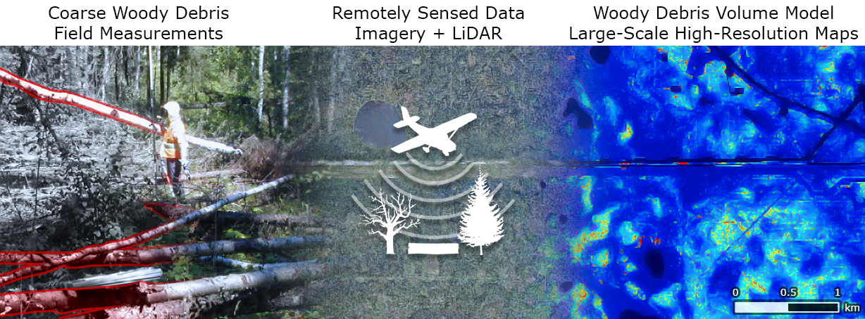
There have been few studies attempting to estimate CWD volumes, including debris as small as 7 cm, accurately and extensively in both visible and occluded areas. The present study aims to address this gap in the literature by developing models which use both GEOBIA-layers and ML information to extract accurate CWD volumes and can be applied to an extensive study area in a boreal forest of northeastern Alberta, Canada. We expected this approach to be able to accurately quantify CWD volume based on field data and we believed that ML data would be beneficial to predictions on occluded areas. Variables we predicted would have a relationship with occurrence and quantities of CWD include the height of trees, active and passive vegetation indices, canopy cover, presence of visible CWD, shadows, water, and wetlands. We tested our models both in a calibration area, where the models were developed, and in a verification area 4 km from the calibration area, and compared the best models using ML variables with the best models without ML variables to assess the impact of infra-canopy information on volume estimation accuracy. We then generated a series of CWD-volume maps designed to illustrate the utility of our approach to aid forest restoration efforts and fire-hazard assessments.

2. Materials and Methods

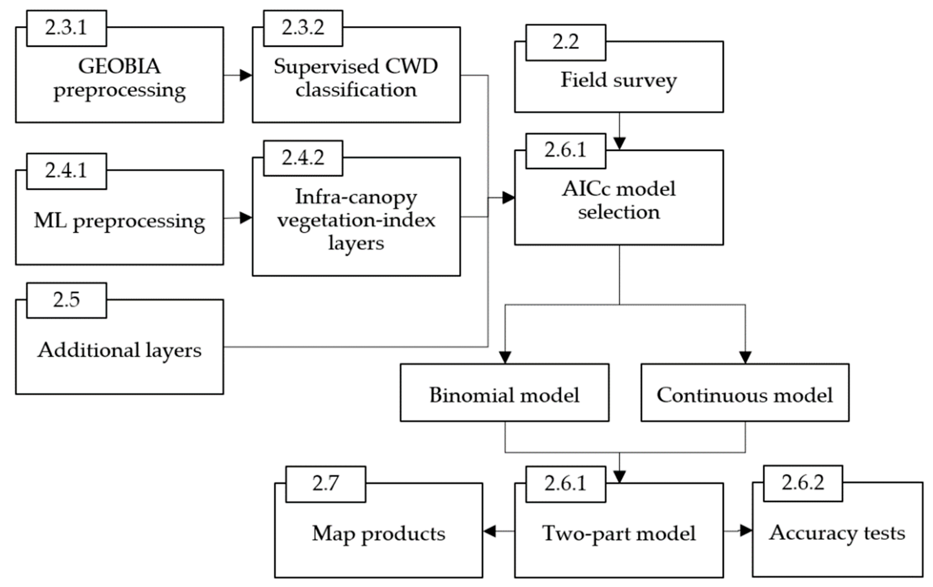
We used 5-cm ground sampling distance (GSD) aerial photos in a geographic object-based image analysis (GEOBIA) workflow to produce a visible CWD layer and then processed multispectral LiDAR (ML) point clouds to produce ground-level vegetation indices layers that allowed for better estimates of occluded CWD quantities. By joining the GEOBIA-derived and ML-derived datasets together, we achieved CWD-volume models with better predictive power than what was possible with GEOBIA alone. Our workflow is summarized in Figure 1 and described in the following subsections.

2.1. Study Area

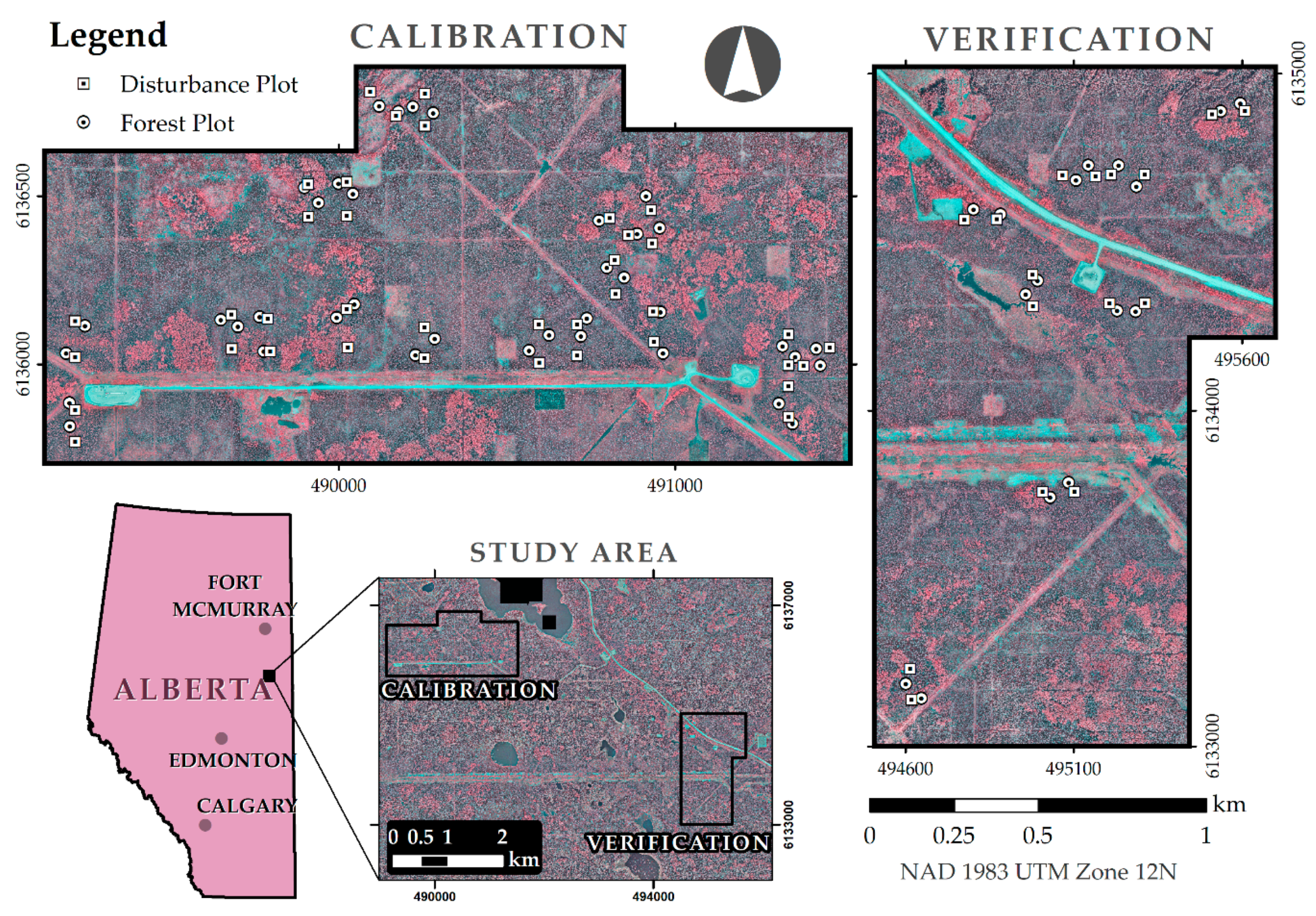
The 4300-hectare study area (Figure 2) is located in the mixed-wood natural subregion of the boreal forest [23] in northeastern Alberta, Canada. The rolling terrain can be divided into two distinct environments: uplands and lowlands (i.e., wetlands). The tree population in the upland areas is mostly composed of jack pine (39.5%; Pinus banksiana Lamb.), black spruce (32.6%; Picea mariana (Mill.) B.S.P.), and trembling aspen (22.2%; Populus tremuloides Michx.) trees. Uplands are composed of 56% coniferous, 12% broadleaf, and 32% mixed forest stands [24] while lowlands are mostly composed of fens (83%), but also include swamps (12%), bogs (2%), and marshes (2%) [25]. Wetlands are dominated by black spruce (64.8%) and tamarack (26.0%; Larix laricina (Du Roi) K. Koch) [24] but can also be mostly composed of shrubs, grasses and moss [26]. There are approximately 342 km of seismic lines (i.e. petroleum exploration corridors; manually digitized) within this area, most of which are visible from aerial images as seen in Figure 2. There are a few (less than 2% of the study area) deactivated timber-harvest sites in the area from the last two decades. Some water bodies and human-made features such as power-lines, constructions, and roads also exist within the study area.

An estimate of canopy closure on the study area, obtained using a LiDAR-derived CHM, revealed that forest stands are much denser on uplands (68.4% average canopy closure) than lowlands (27.2% average canopy closure), as seen in

Table 1. Mean canopy closure on vegetated portions of the study area (averaged stands within the 4300-hectare area). Uplands are divided into forest stand types [24] and lowlands into wetland classes [25].

	Type	Area %	Mean Canopy Closure
Upland Forest	Broadleaf	7%	87%
	Mixed	19%	74%
	Coniferous	33%	61%
Lowland	Swamp	5%	38%
	Fen	35%	27%
	Bog	1%	11%
	Marsh	1%	1%

.

CWD is present in variable quantities on the undisturbed forest and is usually absent on seismic lines. This is the case because historically seismic lines have been constructed by tractors as vegetation-free corridors and all CWD were removed in order to prevent wildfires, only recently CWD have been reincorporated to seismic line management due to their ecological value [7,27]. Many of the seismic lines in the region have not received any restoration treatment, and consequently have low quantities of CWD or no CWD at all. Some seismic lines have been subjected to CWD treatment designed to limit the movement of humans and predators of threatened woodland caribou (Rangifer tarandus caribou) across the landscape [7], which usually can be encountered with isolated piles of CWD and occasionally with entire sections covered by CWD (i.e. complete rollback). This study area was selected for being a representative portion of its natural subregion, with a variety of coniferous, deciduous and mixed forest stands, as well as lowlands containing fens and bogs [25].

We selected two smaller areas for sampling within the 4300-hectare study area, which we denominated calibration and verification areas, respectively (Figure 2). The selection process was mainly based on accessibility and on a representative sample of the forest composition of the overall study area. The calibration area is a 246-hectare area designed to provide training data for our CWD volume models. The verification area is a 209-hectare area designed to provide independent testing data to assess the extensibility of models developed with calibration area data.

2.2. CWD Survey

During the summer of 2018, a field survey was performed within the study area to acquire CWD volume information on both the calibration and verification areas. Given the interest in quantifying CWD in a disturbed environment, with and without restoration efforts, as well as in the unaffected forest, we selected study sites based on the location of seismic lines. Based on this strategy sampling plots could be located within the disturbed line and in the adjacent forest. 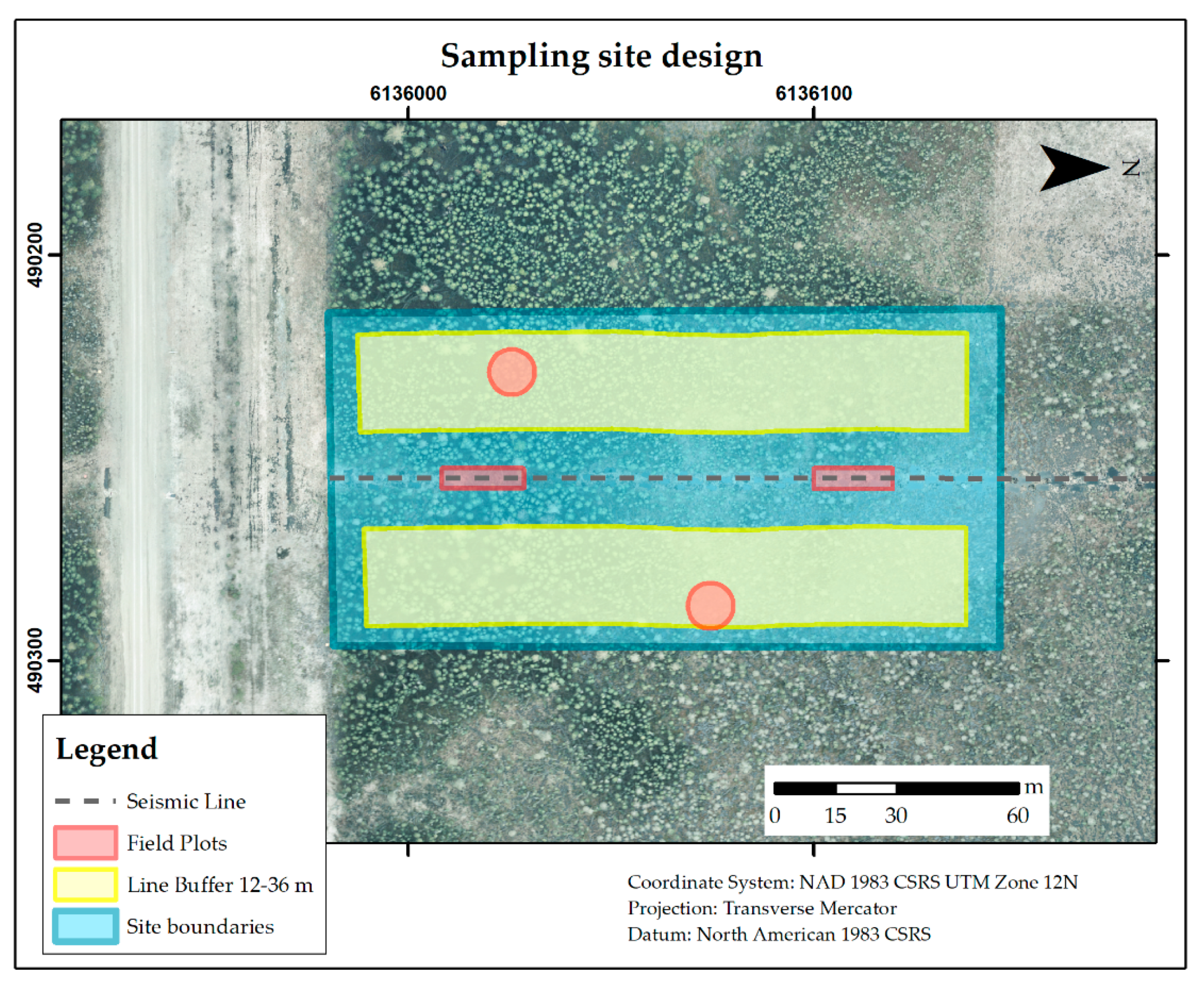To collect a representative sample of CWD in the study area under various natural and artificial conditions, we adopted a stratified-random sampling strategy to select study sites based on the following variables: seismic-line treatment type, surrounding forest tree composition according to Alberta’s vegetation inventory [24], and crown closure. The authors note that despite efforts to achieve a representative sample, given the difficulty in accessing remote portions of the study area and limited time and resources, the site-selection process was constrained by accessibility. The following paragraphs describe overall sampling design and strategy; for more details and figures see Appendix A.

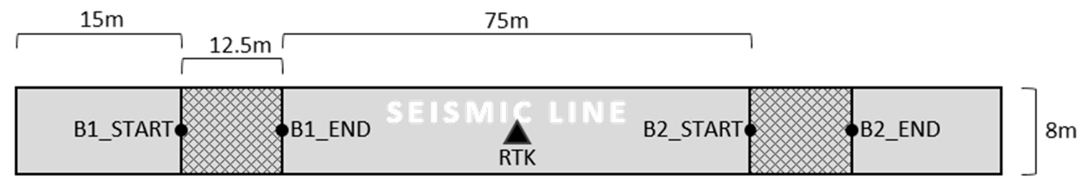
We expected to collect about 100 samples, four from each site, but included more potential sites (35 total) in case there was spare time to collect additional samples or if there were any problems with the visited sites. For each site, we selected four 100 m² plots for sampling CWD volume. To obtain data in both natural and altered sites, while avoiding transitions between either, two plots were located on the seismic line and two plots were located in the surrounding forest. We call the plots in the seismic line “disturbance plots”, and they were designed to be rectangular areas limited by the footprint of the disturbance, with width equal to the seismic line’s width and variable length to obtain a 100 m² area. The plots in the surrounding natural environment were denominated “forest plots”, and they were circular areas with a radius of 5.64 meters. We positioned the disturbance plots systematically, one of them starting 15 meters away from the beginning of the line, and the other positioned starting 75 meters away from the end of the former disturbance plot. Finally, the forest plots were positioned randomly, with their center point located within a minimum distance of 12 meters and a maximum distance of 36 meters away from the center of the seismic line. By the end of the field season, we had sampled a total of 108 plots: 76 plots (19 sites) in the calibration area and 32 plots (8 sites) in the verification area.

Each plot was located and positioned using a real-time kinematic (RTK) global navigation satellite system (GNSS, Trimble R8 - Trimble, Sunnyvale, United States) with average horizontal precision of 4.57 cm, then every piece of CWD present within the plot was examined and measured for volume. In each plot, the volume measurements were restricted by the extent of the plot boundaries, and any CWD crossing a boundary was considered as if it ended at the edge of the plot. CWD was defined as dead wood, either intact or partially decomposed, with at least 7 cm of diameter at the largest end and at least 1 meter of length. The 7-cm diameter threshold was chosen for being a common choice in the literature and given that the majority of woody debris, especially those encountered in the lowland portions of the study area, did not surpass 10 cm in diameter. Any CWD positioned horizontally or leaning with an angle larger than 45° relative to vertical surface was classified as a log and was measured as part of the total CWD volume per plot presented in this study. Any CWD positioned vertically or leaning with an angle smaller than 45° was classified as a snag and was also measured but is not considered for the CWD volume per plot presented in this study, since the map products presented here mainly target seismic line restoration and fire-hazard assessment studies, which usually show little interest for snags.

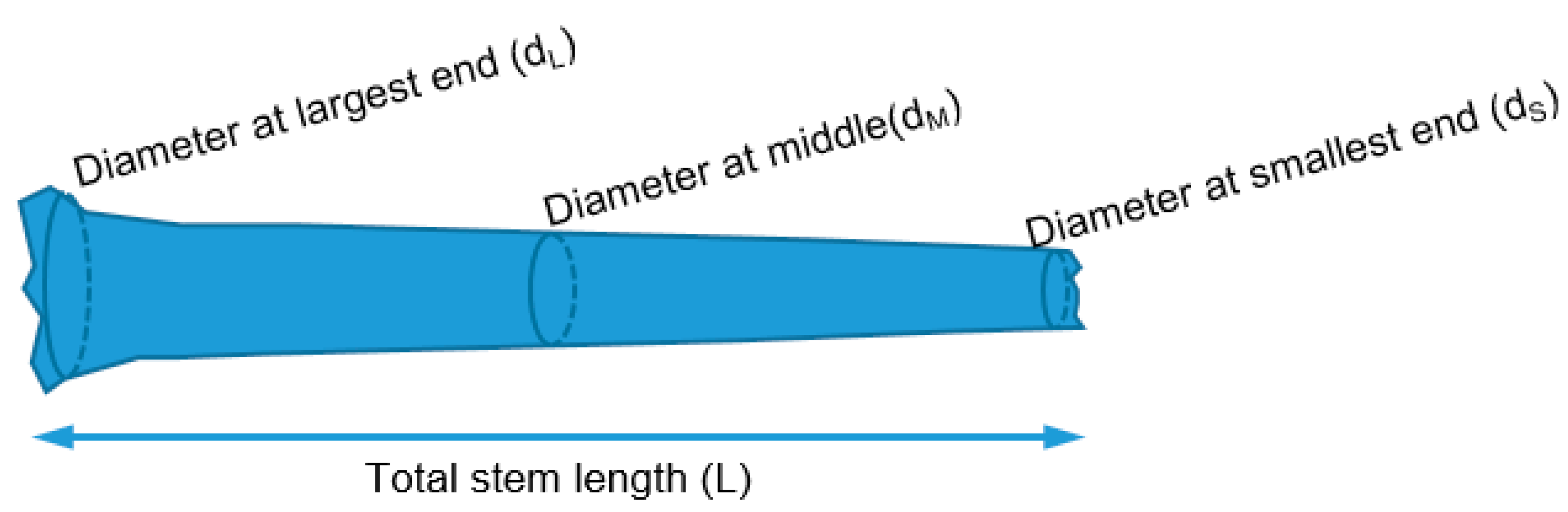
Log volume was derived from three diameter measurements, one obtained at each end and one obtained in the center of the extent of the log, as well as the total stem length in meters. Volume was calculated using Newton’s formula, which accounts for the tapering shape of the log [28]:

$$V=\frac{L}{6}\left(\pi {\left(\frac{d_L}{2}\right)}^2+4\pi {\left(\frac{d_M}{2}\right)}^2+\pi {\left(\frac{d_S}{2}\right)}^2\right)$$

(1)

where V is the volume of the main stem, d_L is the diameter measured at the largest end, d_M is the diameter at the middle, d_S is the diameter at the smallest end, and L is the length of the stem.

Additional data recorded per CWD piece within each plot included: state of decay, species, azimuth, and inclination. Furthermore, canopy closure was recorded at the center of each plot via hemispherical photography. Initial tests with these variables did not yield any particularly useful insights or predictions. For the purposes of this study, these metrics were discarded save to confirm that our sample of CWD volume was representative of a good variety of states of decay, species, and canopy closure.

Once data were collected in the study area, the volume per plot was calculated by summing up the total volumes of all pieces measured within. Every plot was integrated into a geodatabase according to its size, position, and orientation obtained in the field with RTK measurements, and its respective total CWD volume. We had to remove three plots from the verification area from analysis since one of them could not be positioned properly with the RTK and two of them changed significantly since the remote sensing data were captured: one was a forest in aerial images and became clear-cut when sampled, and the other contained a recently felled, large tree not captured in the remote sensing data.

2.3. Remote Sensing and Pre-Processing

Two different data collection missions were performed to obtain the remote sensing data over the study area: one during the summer of 2017, which captured high resolution (5-cm pixel-size) visible and near-infrared spectrum images as well as a dense LiDAR point cloud (40 pts/m²), and another during the summer of 2018, which captured multispectral LiDAR (ML) data with lower point density (raw 11 pts/m²). The data collected during the 2017 mission were used in a geographic object-based image analysis (GEOBIA) workflow to locate visible CWD objects (vCWD), and the 2018 ML data was used to generate infra-canopy vegetation indices useful as indicators for occluded CWD quantity. GEOBIA consists of subdividing georeferenced input images into segments denominated “image-objects”: relatively internally homogenous segments of the image usually defined by contrasts around their edges, which are intended to represent distinct parts of real-world objects [29]. We acknowledge the temporal disconnect between the dates of the field work and first LiDAR mission (2017) and second LiDAR mission. It is our assumption that any changes in CWD volume within that time period were minor and had no significant impact on our study.

2.3.1. Orthomosaics and Dense LiDAR Point Cloud

The remote-sensing datasets used in the GEOBIA portion of this study were obtained prior to field data collection via a piloted aircraft mission performed by OGL Engineering of Calgary (Orthoshop Geomatics Ltd., Calgary, AB, Canada) between August 2 and 4, 2017. The Cessna 210T aircraft used in this mission, flying at 67 m/s 850 m above ground, carried an optical sensor, a LiDAR sensor, a GNSS, and an inertial measurement unit. The flight path obtained 5.5 cm ground sampling distance (GSD) images with 80% forward overlap and 60% side overlap. We deployed 250 visible ground control points (GCP, 60 cm squares with a bullseye marking) prior to the flight and measured their locations with an RTK GNSS (8 mm horizontal and 15 mm vertical precision). We used 100 of these targets for georeferencing purposes and the remaining 150 for accuracy assessment. The final products had X, Y, and Z had accuracies of 5, 10, and 11 cm, respectively.

OGL Engineering treated the raw LiDAR point cloud, with a point density of approximately 40 pts/m², for noise removal and ground-point classification using Terrasolid software. Using ESRI (Environmental Systems Research Institute) ArcMAP (version 10.6.1; ESRI, Redlands, CA, USA), we gridded the elevation of the ground points into a 25cm GSD digital terrain model (DTM), and of the first return points into a 25 cm GSD digital surface model (DSM). A canopy height model (CHM) was obtained by subtracting the DSM by the DTM. We generated a 5 cm GSD orthomosaic of the study area by processing the air photos in Pix4Dmapper [30,31], using standard procedures for photo alignment, georeferencing and adjustments using a photogrammetric point cloud. A normalized difference vegetation index (NDVI) raster layer was generated using the near-infrared (NIR) and red bands of the orthomosaic.

2.3.2. Multispectral LiDAR Acquisition and Processing

Since the study area is densely vegetated, much of the CWD measured in field plots was not visible in aerial images. For this reason, multispectral LiDAR (ML) data were used to obtain the intensity information of locations under the canopy, which were then used to derive sub-canopy vegetation indices. ML-derived vegetation indices have been shown to approximate passive imagery vegetation indices such as NDVI and normalized burn ratio (NBR) [20]. In the following sections, LiDAR-derived vegetation indices will be referred to as active vegetation indices.

ML data were collected over the study area by the University of Lethbridge ARTEMiS lab (Advanced Resolution Terradynamics Monitoring System Laboratory), during a piloted flight mission performed on July 23th of 2018, concurrently to the field data collection. The ML sensor used was a Titan (Teledyne Optech, Toronto, ON, Canada) unit, which simultaneously captures three wavelengths: 1550, 1064, and 532 nm, hereby referenced as short-wave infrared (SWIR), near infrared (NIR), and green channels, respectively. The Piper Navajo aircraft used in this mission flew at 65 m/s, 1000 m above ground, with a planned side overlap of 50% and planned pulse density of 3 pts/m² per channel. The raw LiDAR data were calibrated using LiDAR Mapping Suite [32] by the ARTEMiS lab, who reported 12 cm horizontal and 5 cm vertical RMSE strip-to-strip accuracy. The ML datasets for all three channels was supplied in 54 separate tiles of the study area.

The following procedures were performed with LAStools [33] and ArcMap [30] software. Overall point density and number of points per return of the ML datasets on the study area were calculated using the lasinfo tool: 1.51 pts/m², 4.49 pts/m² and 5.00 pts/m² for the Green, NIR and SWIR channels respectively. The percentage of single returns was of 99.7%, 33.5%, and 27.5% respectively for these channels. Rain previous to the flight and wet ground likely caused attenuation losses on all channels, most notably the green channel, which is obtained with a larger beam divergence and higher tilt angle than the other channels and is expected to have higher losses below the canopy [21]. Point height relative to ground was obtained on each channel with lasground (wilderness setting), which is a tool based on Axelsson’s [34] triangular irregular network filtering algorithm. Then, to avoid outliers, the maximum intensity of the ground points was set to three standard deviations plus the mean, according to the intensity distribution of each channel. Points with an estimated height smaller than 1 meter were exported in “shapefile” (SHP) format using las2shp. The point intensity of each SHP file was gridded into raster images using the inverse distance weighted (IDW) tool in ArcMap, with a cell-size of 50 cm, a fixed search radius of 1 meter and minimum of 2 sample points. IDW were used to reduce some of the bias of gridding and cell spatial attribution and was selected over simpler averaging methods because it preserved some of the variance of the raw datasets. IDW also was useful in reducing the effect of noise and banding, which was especially observed in the NIR channel, where the intensity distribution was offset between scanline directions due to internal hardware misalignment issues with the sensor (2.3%, 3.4%, and 0.2% average banding for the SWIR, NIR, and green channels respectively). Due to the small percentage of single returns, mostly observed in vegetated areas, all returns were considered in this study despite the fact that this introduces noise in the data [21]. Using the intensity raster images for each ML channel, active NDVI (aNDVI) and active NBR (aNBR) layers were calculated using the raster calculator tool in ArcMap. The green channel was used for aNDVI as a visible-spectrum substitute for the traditionally used red channel on passive NDVI calculations. Both aNDVI and aNBR layers were later used to derive vegetation-indices metrics per 100 m² plots, which were included in CWD volume models as predictor variables. The individual ML channels were not included in the analysis as it was assumed that active vegetation indices represented more parsimonious variables, likely to retain the information of multiple spectral layers.

2.4. Geographic Object-Based Image Analysis

We created a visible-CWD (vCWD) raster image over the study area by processing aerial images as well as LiDAR data via a GEOBIA workflow, involving machine-learning “random forest” supervised classification. This process was described in detail by Lopes Queiroz et al. [12]. All spectral bands from the orthomosaic and the NDVI layer, generated with the 2017 mission data, were used to segment the study area into image-objects using eCognition [35]. We used the following parameters: scale 10, shape 0.6, and compactness 0.4. All layers used to segment the study area, as well as the CHM layer, were used to train a random forest (RF) machine-learning classifier.

Random forest supervised classification involves providing a set of training samples, in this case CWD image-objects as well as other broad types of features present in the landscape, to a RF classifier which uses the training data as reference to create a set (forest) of classification trees, each tree with randomly selected input variables [36]. A trained RF was applied to classify all image-objects in the study area and identify the CWD objects visible on aerial images.

Classifier Training and Application

To create a reference dataset for RF classification, 5000 randomly selected image-objects over the calibration area were manually classified into five distinct classes: log, snag, water, dirt, and other. The selection of the reference objects was stratified around NDVI: 20% of samples from objects with NDVI greater than −0.1 in the NDVI image and 80% of samples from objects with NDVI smaller than −0.1. This strategy was adopted given that the clear majority of identified CWD objects had an NDVI lower than that threshold and that CWD are very infrequent when compared to the other object classes. A portion of these reference objects could not be classified due to being indistinct.

The reference dataset on the calibration area had a total of 3710 classified objects, of which 364 were logs. The spatial, spectral and height attributes of these objects were used as predictor variables to train a RF classifier, which was applied to the whole study area in three processing chunks that were later merged together. More details of the reference dataset, as well as about the process used to test and apply the classifier can be found in Lopes Queiroz et al. [12], who reported completeness between 76.9% and 81.5% and correctness between 75.8% and 87.0% for logs in the study area. Completeness is defined as the percentage of true positives relative to all positives in reference data and correctness is defined as a percentage of true positives relative to all positives in testing data.

After the RF classifier was applied to the whole study area, a planimetric map layer of visible CWD was generated by marking all 5 cm raster cells within image-objects classified as log. Some groundcover features not included in training the classifier but present in the larger study area, such as water bodies, construction, and parking lots, were manually removed from the final product. This layer was later used to derive visible CWD area per 100 m² plots, which was included in CWD volume models as a predictor variable.

2.5. Additional Layers

Aside from the vCWD layer generated from GEOBIA, and the aNDVI and aNBR layers generated from ML, we produced additional layers for consideration as predictor variables in CWD volume models.

The main factors we associated to occlusions of CWD on aerial images were canopy cover, tall grass, and heavy shadow. In an attempt to account for these factors, we generated canopy cover (CC), passive NDVI (pNDVI), and brightness layers, respectively. The CHM used in GEOBIA was classified into canopy and non-canopy pixels by selecting all cells with heights greater than 2m above the ground. This layer was later used as a proxy for canopy cover in the CWD volume models. The pNDVI layer used in GEOBIA was considered as a candidate predictor variable in the CWD volume models. A brightness layer was generated by averaging the visible-spectrum (RGB) intensities of the orthomosaic used in GEOBIA.

Factors we associated to broad-scale CWD volume variance and distribution on the study area were: the spatial distribution of wetlands and uplands, and of the height of the alive trees. A visible-water area (vWater) layer was generated by selecting the image-objects classified as water by the RF classifier. Another proxy for wetland distribution we used was a wetland probability (WP) layer obtained from ABMI [37]. Finally, the CHM used in GEOBIA was selected to extract metrics of tree height per 100 m² plots.

2.6. Model Selection

Each of the 108 field-plot polygons were attributed with variables from the following layers: vCWD, aNBR, aNDVI, CC, pNDVI, Brightness, vWater, WP and CHM. Using the zonal statistics tool from ArcMap the following statistics were extracted for each layer on each plot: minimum, maximum, range, mean, standard deviation and sum. Given that there were many potential predictor variables, six metrics for each one of eight layers, a model selection strategy was adopted using Akaike’s Information criterion (AIC), while discarding highly correlated variables (R > 0.6). Summary statistics of all remaining variables, after the correlated variables were discarded, are presented in

Table 2. Description and summary statistics of all variables used in model selection, each variable summarized with: mean, standard deviation (Std Dev), minimum (Min) and maximum (Max). The response variable was coarse woody debris (CWD) volume measured in the field, and the predictor variables were derived from a variety of remote sensing products. Visible CWD (vCWD) and water (vWater) area were derived from the results of geographical object-based image analysis (GEOBIA) on aerial orthophotos obtained over the study area. A wetland probability raster was obtained from ABMI [37]. Canopy closure (CC) was derived from a canopy height model (CHM). Passive normalized difference vegetation index (NDVI) was derived from the orthophotos used in GEOBIA, while active NDVI and normalized burn ratio (NBR) were derived from multispectral LiDAR datasets.

Variable	Definition	Mean	Std Dev	Min	Max
Response	Response variable: total ground-truth CWD volume (m3).	0.25	0.34	0.00	1.50
vCWD	Total visible CWD area (m2) on orthophotos, obtained with GEOBIA.	1.50	2.63	0.00	11.89
vWater	Total visible water area (m2) on orthophotos obtained with GEOBIA.	1.31	3.00	0.00	14.40
Brightness	Average visible-spectrum reflectance on orthophotos. Scaled 0–255.	99.06	10.24	75.33	122.11
WP	Average wetland probability, scaled from 0 to 1.	0.28	0.30	0.02	0.92
CC	Canopy closure, obtained as proportion of cells with CHM > 2 m.	0.45	0.31	0.01	0.96
CHMmax	Maximum CHM value within plot (i.e. height of tallest tree).	14.97	5.47	2.72	30.82
pNDVIr	Passive NDVI range within plot.	0.99	0.17	0.57	1.37
pNDVIsd	Passive NDVI standard deviation within plot.	0.14	0.04	0.06	0.27
aNDVIr	Active NDVI range within plot.	0.95	0.24	0.00	1.72
aNBRr	Active NBR range within plot.	1.49	0.18	0.51	1.82
aNBRsd	Active NDVI standard deviation within plot.	0.26	0.07	0.09	0.43

. All procedures for model selection and validation we performed in R (version 3.5.1; R Core Team, 2018).

2.6.1. CWD Volume Modelling

CWD quantities are known to be positively skewed and not normally distributed [1]. Since we found CWD volume distribution on 100 m² plots to follow this pattern, as well as zero-inflated, CWD volume was modeled in two parts: a binomial distribution for the presence/absence of CWD, and a continuous distribution for volume on the plots where CWD was present. A binary response variable was created for the binomial models by treating all plots where CWD was absent as zero and all plots where CWD was present as one. The continuous model was trained on plots where CWD was present and used CWD volume as response variable. Candidate models were selected separately for the binomial and continuous parts, then combined into two-part CWD volume models. The final predicted CWD volume according to two-part models equals the predicted binomial component times the predicted continuous value. Given that the distribution of CWD volume in our study plots was positively skewed as well as zero-inflated, zero-adjusted gamma (ZAGA) distribution models were used to incorporate the best continuous and binomial models. We used the generalized additive models for location, scale and shape (GAMLSS) library in R to generate and test our ZAGA models [38,39]. Generalized additive models (GAMs) allow for the response variable to be modelled with Gaussian as well as numerous non-Gaussian distributions, as opposed to traditional linear modelling, and allow for link functions to model the relationship between the response variable and the predictors [40]. Additionally, GAMs are well suited for modeling non-linear relationships between the response and predictor variables because they are built based on the structure of the reference datasets instead of assuming a previously selected linear distribution [41]. The main assumptions of GAMs are that the samples are statistically independent, the variance and link functions are selected correctly, and that there are no outliers influencing the fit [42]. The stratified-random sampling strategy adopted in this study, as well as statistical tests and investigation performed with the raw data in R ensured the selected ZAGA models follow these assumptions.

Small-sample AIC (AICc) is a useful indicator for model selection when dealing with multiple potential models created with a small sample-size [43]. Early tests with regular AIC revealed that CWD volume models using our field data were consistently overfitted, and therefore AICc was used instead. Model selection tables were generated for CWD volume two-part linear models using the candidate variables as predictor variables. Models were candidates only if their delta AICc (ΔAICc, calculated as AICc difference from the model with the smallest AICc) was smaller than 2, which is commonly used as a threshold for model selection in the literature [43]. Many of the predictor variables were highly correlated, with Pearson’s R greater than 0.6. In these cases, only the variable that was most often present in candidate models was maintained, and other correlated variables were discarded. Candidate models were selected with and without ML variables for comparison. All possible combinations of candidate binomial and candidate continuous models were tested as ZAGA models, of which only the models with ΔAICc smaller than 2 were considered as our final candidate models for CWD volume.

2.6.2. Keep-One-Out Cross-Validation and Verification Tests

To test the accuracy and extensibility of the candidate models, the predicted CWD volume according to the two-part model was regressed against the actual CWD volume measured in the field plots to calculate R2 and RMSE values. A keep-one-out cross validation test was performed in the calibration area by training the models once for every plot in the area using all the calibration data except for each plot where a CWD volume prediction was generated. Another test was executed by training the models using the calibration area data and applying them to predict CWD volume on the verification area plots. Finally, we tested the accuracy of predicted CWD ground cover (m²) derived from the vCWD layer versus CWD measured ground cover per plot, without any additional modelling, to assess the potential and limitations of GEOBIA of CWD.

2.7. Map Production

Among all candidate models for CWD volume, we selected a two-part model with the greatest predictive power as a preferred model. The preferred model included both image analysis and multispectral LiDAR (ML)-derived variables and is described in the following sections of this document. Given that the ML layers contained a few void cells, the preferred model was only applied on 100 m² cells containing at least 50% coverage of the aNBR layer, which accounts for 99.3% of the study area (excluding water bodies and human-made features). On cells with less than 50% coverage on the aNBR layer (0.7% of the study area), we used the best model not containing ML variables.

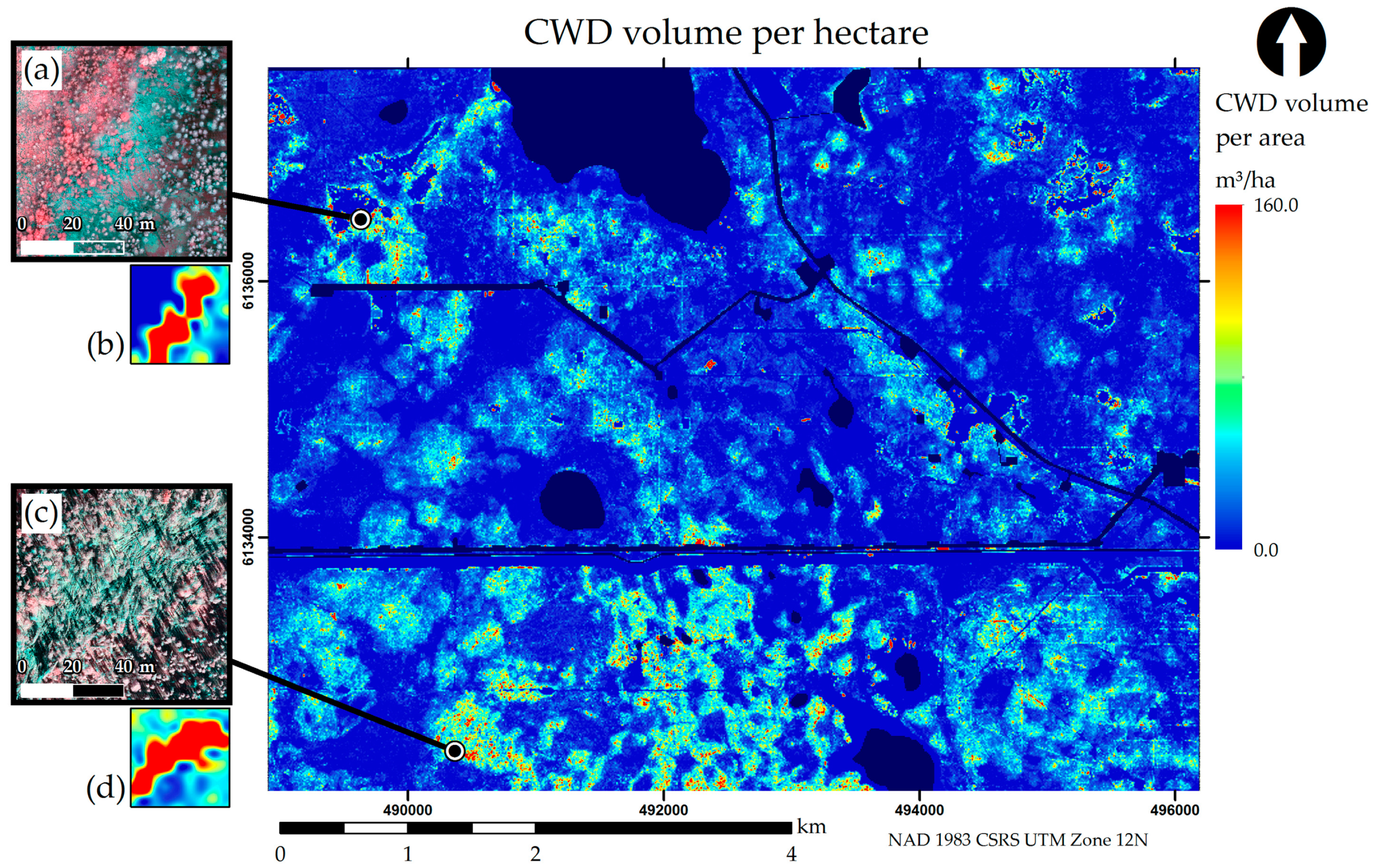
Given the best models selected for CWD volume estimation according to the tests and specifications previously discussed, we generated two map products of CWD volume per hectare (m³/ha) on the entire 4300-hectare study area: one map dedicated to comprehensive CWD volume across all land cover types, and another dedicated to seismic line CWD density. Since the ML layers contained many gaps due to lower ground return density on closed canopy areas, the best-performing model using ML layers was used as a preferred model to generate these maps, and the best performing model without ML layers was used as a fallback model.

2.7.1. Overall CWD Volume Layer

The 4300-hectare study area was gridded into 10 × 10 m cells using the fishnet tool in ArcMap, and each cell was attributed with values from all relevant predictor layers using the zonal statistics tool. Water bodies and human-made features accounted for 7.5% of the study area. These were removed from further analysis, given that these land-cover types were not accounted for when training the models. The attribute table containing predictor variables for all cells, as well as their individual latitude and longitude, was extracted as a comma-separated values (CSV) file and imported into R. The ZAGA models trained with the calibration data were applied to all cells generating CWD volume predictions for the entire study area. These predictions were multiplied by 100 to obtain an estimate of volume per hectare as opposed to volume per 100 m². Given that there were a few (less than 0.05% of the data) overpredictions well above the range of CWD volume observed in field plots, the maximum prediction value was set to the mean plus four standard deviations of the field sample distribution (~160 m³/ha). Predictions, along with their geo-locations, were imported into ArcMap as points and rasterized using the “point to raster” tool.

2.7.2. Seismic Line CWD Volume Layer

Using the CWD volume layer created for the entire 4300-hectare study area described above, segments of seismic lines of the study area were attributed with their mean CWD m³/ha. A vector layer of all seismic lines on the study area was obtained via a seismic line mapper tool [44], which uses a least-cost path solution on a CHM to trace linear features on forested environments. The “generate points along lines” tool in ArcMap was used to both generate dense sampling points as well as sparse split points to segment each seismic line. Sampling points were attributed using the “extract values to points” tool, extracting values from the raster of overall volume. Lines were split into segments using the “split line at point” tool. Finally, segments were attributed with their mean CWD volume using the “spatial join” tool to link values of sampling points with each line segment.

3. Results

3.1. Accuracy of Best Models

The accuracies of the best model using ML data and of the best model without ML data were tested both on the calibration area using keep-one-out cross-validation (0.623 R², 0.224 RMSE using ML data; 0.514 R², 0.254 RMSE without ML) and on the verification area while training only on calibration area samples (0.721 R², 0.198 RMSE using ML data; 0.628 R², 0.203 RMSE without ML). Goodness of fit (R²) and root mean square error (RMSE) were comparable between cross-validation tests in the calibration area and tests in the verification area. Furthermore, these metrics were better in models including ML variables in relation to models without ML variables. The regression line of all models approximates the 1:1 relationship with a slightly gentler slope. The variance of CWD volume was greater in disturbance plots than in forest plots, and the former also displayed stronger zero-inflation in the calibration area plots (Figure 3).

3.2. Map Products

To showcase the application of the selected models, CWD volume per hectare (m³/ha) was mapped over the 4300-hectare study area to generate two map products: a comprehensive map over all ground-cover types with 100m² raster cell-size (Figure 4), and a map of seismic line 100-m segments classified according to their average CWD density (Figure 5). High density CWD clusters were detected at the edges of previously harvested areas (Figure 4a) and in the southwestern portions of the study area in the form of partial windthrows (Figure 4c). Seismic lines with (Figure 5a) and without (Figure 5c) CWD treatment were identified in the maps. In Figure 4b, very low CWD quantities are observed in the interior of the harvested area (northwestern portion of Figure 4a), moderate CWD quantities in the natural forest (southeastern portion of Figure 4a), and very high CWD quantities in the transition between the two.

CWD volume in the reference data was compared to the volume in the map products (Figure 4 and Figure 5), which were divided into upland and lowland according to ABMI’s wetland classification layer [25]. These datasets are presented as box-and-whisker plots below (Figure 6). The distribution of CWD volume on the final maps was quite similar to the distribution on forest plots, even when separating the area into lowland and upland, though the upper quartile of the predictions was a bit lower. The average volume in upland was 13.7 m³/ha and in lowland was 3.4 m³/ha. Disturbance plots, most of which were located on treated seismic lines, had much higher volumes than the rest of the study area. This was expected given the practice of creating CWD piles as part of restoration treatments [7]. The population of seismic lines on the map products had slightly lower volumes than the rest of the upland areas, but treated lines had much higher volumes than untreated lines. Average volume on treated and untreated seismic lines was 18.2 m³/ha and 9.4 m³/ha respectively.

3.3. Model Selection Tables

The model-selection table for the candidate ZAGA CWD volume models (

Table 3. Candidate two-part models for coarse woody debris (CWD) volume according to small sample Akaike information criterion (AICc). The rank (r), degrees of freedom (df) and delta AICc (ΔAICc) are provided for each model. The following variables were selected in all continuous models: area of detected CWD objects via image-analysis (vCWD); canopy closure (CC); and height of the tallest tree (CHM_max). The following were selected in some continuous models: standard deviation of the active normalized burn ratio (aNBR_sd) and range of passive NDVI (pNDVI_r). Finally, all logistic models included: vCWD, standard deviation of passive NDVI (pNDVI_sd), visible water area (vWater) and wetland probability (WP).

r	Continuous Model	Logistic Model	df	AICc	ΔAICc
1	vCWD2 + CC + CHMmax + CHMmax2 + aNBRsd2	vCWD + pNDVIsd + vWater + WP	12	−2.08	0.00
2	vCWD2 + CC + CHMmax + CHMmax2 + aNBRsd2 + pNDVIr	vCWD + pNDVIsd + vWater + WP	13	−1.98	0.09
3	vCWD2 + CC + CHMmax + CHMmax2 + pNDVIr	vCWD + pNDVIsd + vWater + WP	12	−1.43	0.64
4	vCWD2 + CC + CHMmax + CHMmax2	vCWD + pNDVIsd + vWater + WP	11	−0.43	1.65

) is presented below. It is noteworthy that all candidate models shared the same logistic component: a model containing vCWD, pNDVI, vWater, and WP variables. The two models with the smallest AICc were models including aNBR, while the two other models did not include any ML variables. All continuous models shared CC, CHM and vCWD variables, and some models included either aNBR or pNDVI. No candidate models selected brightness or aNDVI variables.

Given the results presented in Table 3, model ranked 1 was selected as the best simplest predictive model including ML variables and model ranked 4 was selected as best simplest model excluding ML variables. Models ranked 2 and 3 are variations of these selected models adding pNDVI as a variable, and given all candidate models were “tied” with ΔAICc lower than 2, only the simplest models were chosen for application in the study area.

To better understand the composition of the best ZAGA model, standardized coefficients for the predictors, including multispectral LiDAR, were obtained by modelling scaled predictor variables with a mean of zero and standard deviation of one (

Table 4. Intercept and coefficients for binomial part of the best zero-adjusted gamma model. Values are presented for models created with the original training data and models using standardized predictor variables (mean of zero and standard deviation of one). Variables include visible coarse woody debris area (vCWD), standard deviation of passive normalized difference vegetation index (pNDVI_sd), visible water (vWater) and wetland probability (WP).

	Intercept	vCWD	pNDVIsd	vWater	WP
Original	−0.137	−1.823	−17.701	0.559	4.687
Standardized	−3.674	−5.059	−0.819	1.874	1.333

and

Table 5. Intercept and coefficients for continuous part of the best zero-adjusted gamma model. Values are presented for models created with the original training data and models using standardized predictor variables (mean of zero and standard deviation of one). Variables include squared area of visible coarse woody debris (vCWD), canopy closure (CC), height of tallest tree (CHM_max), squared height of tallest tree (CHM_max²) and squared standard deviation of active normalized burn ratio (aNBR_sd²).

	Intercept	vCWD2	CC	CHMmax	CHMmax2	aNBRsd2
Original	−6.956	0.012	−3.070	0.581	−0.012	11.284
Standardized	−1.547	0.133	−0.662	1.161	−0.369	0.061

). This enabled us to study the relative contribution of each explanatory variable to the final model in terms of strength and direction.

3.4. Accuracy of Visible-CWD Layer

Figure 7 contains graphs comparing ground cover of vCWD image-objects with measured CWD ground cover in field plots, for all calibration area plots as well as for only the plots with negative average pNDVI. Disturbance plots exhibited greater zero-inflation in the response variable than forest plots and both types of plots had zero-inflated predictions. Goodness of fit (R²), RMSE, and slope of regression in plots with negative NDVI were all much superior than these metrics in all field plots.

4. Discussion

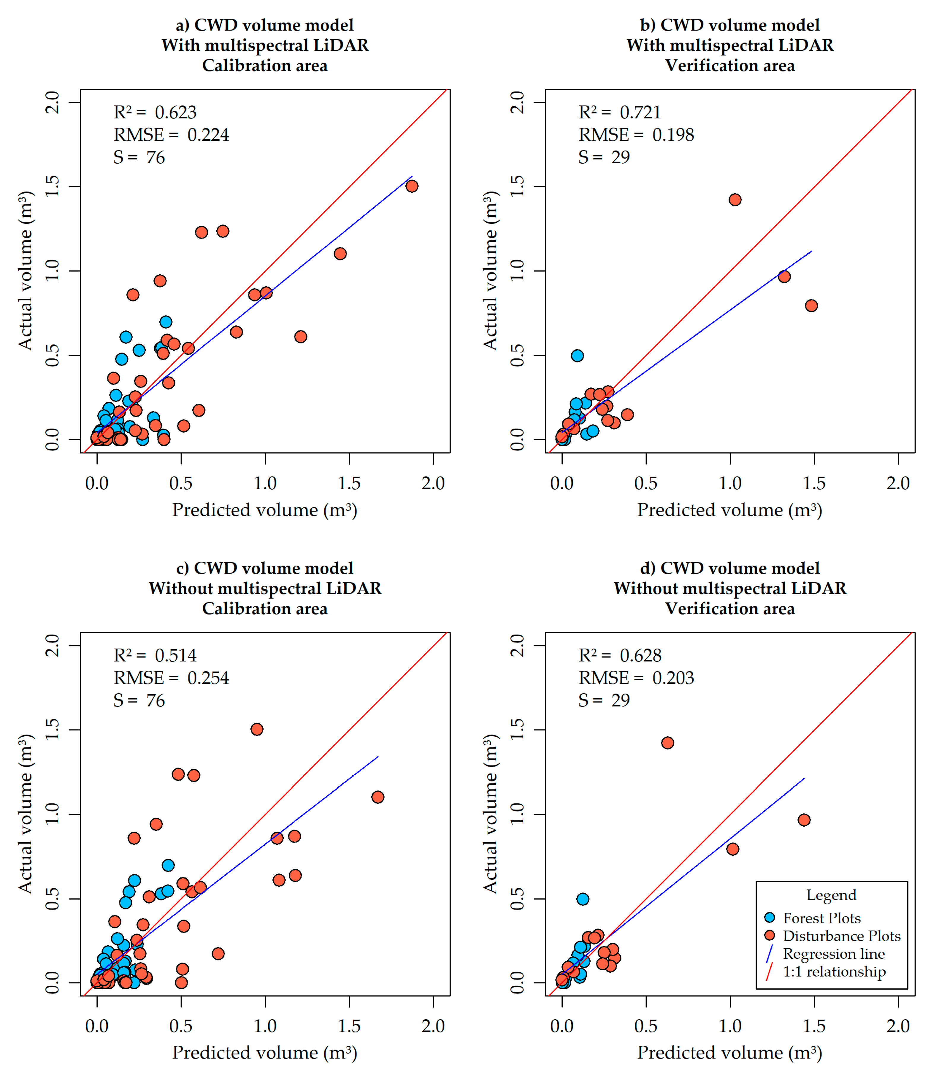
Once a model was selected, the production of map products over the entire area of study was achievable using common map algebra operations in a GIS environment. The selected models achieved good predictive accuracy (0.623 R², 0.224 RMSE in cross-validation; 0.721 R², 0.198 RMSE in the verification area) but required a sophisticated set of inputs, involving high-resolution aerial images, high density LiDAR point clouds as well as ML point clouds. The results presented in Figure 3 indicate that, even where ML data is not available, CWD volume can still be modeled with good predictive accuracy (0.514 R², 0.254 RMSE in cross-validation; 0.628 R², 0.203 RMSE in the verification area), with a mean decrease of 0.101 in R² and a mean increase of 0.0125 in RMSE in relation to ML-inclusive models. 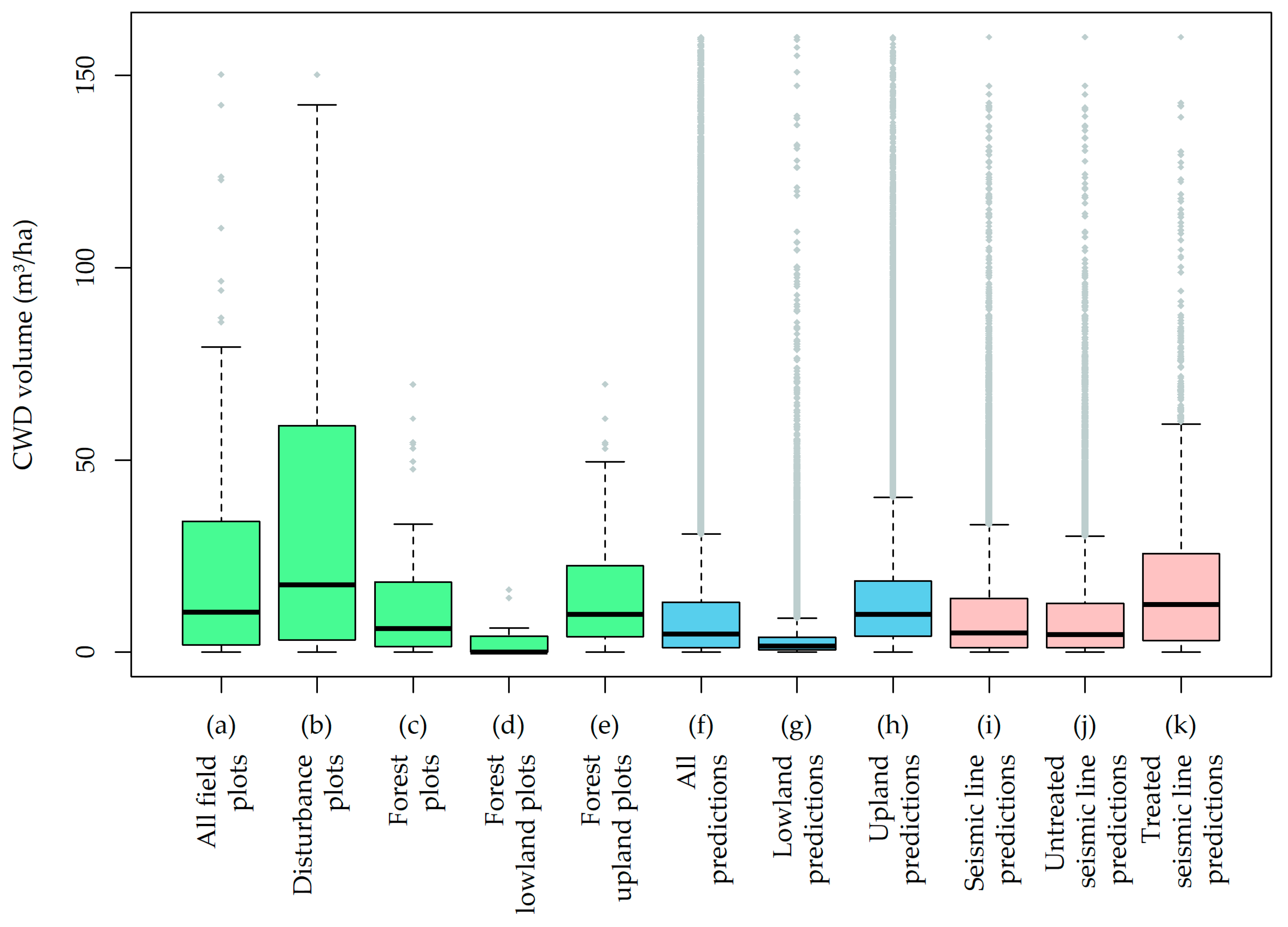The final maps of CWD volume in the study area (Figure 4 and Figure 5) reveal that even though CWD distribution is largely controlled by the occurrence of wetlands, artificial piles of CWD on seismic lines and clear-cuts are exceptions which can cause CWD anomalies. Overall average CWD volume in the study area (9.78 m³/ha for the entire study area, 17.73 m³/ha for uplands and 3.14 m³/ha for lowlands) was small when compared to what Lee et al. [45] measured in aspen-dominated stands in Alberta (108.8 to 124.3 m³/ha), but upland volumes in the present study are comparable to several other studies [46,47,48] in boreal forests as presented in

Table 6. Minimum and maximum average coarse woody debris volume (m³/ha) over varied boreal forest types presented in other studies. Note that the present study estimated volumes in 100 m² plots and upscaled the values for an estimate per hectare. Minimum value from Pedlar et al. [48] includes snags. Sturtevant et al. [46] values are for individual stands, while all other studies present averages.

Citation	Forest Types (Min/Max)	Location	Min	Max
Lee et al., 1997 [45]	20–30 yr. aspen stands/120 + yr. aspen stands	AB, Canada	108.8	124.3
Linder et al., 1997 [49]	Natural pine, spruce and deciduous stands	Sweden	62	-
Sturtevant et al., 1997 [46]	58 yr. fir stand/80 yr. fir stand	NL, Canada	15.2	78.1
Sippola et al., 1998 [47]	Managed 15 yr. spruce stands/Natural mixed stands	Finland	6.6	47.2
Pedlar et al., 2002 [48]	Spruce stands/mixed stands	ON, Canada	<17.8	131.5
Present study	Black spruce dominated wetlands/Upland coniferous, deciduous and mixed forests	AB, Canada	3.14	17.73

. It is not surprising that lowlands had a very low volume of CWD (3.14 m³/ha) since the lowland trees observed in the field were small (commonly close to 7 cm diameter at largest end) and since not all wetlands were densely populated by trees, especially bogs and marshes which were mostly shrubby. Additionally, the CWD distribution on the produced maps was very similar to the distribution in the reference data (Figure 6), with mean values from uplands and lowlands in the reference data (17.7 and 3.1 m³/ha respectively) close to the mean of uplands and lowlands in the final maps (13.7 and 3.4 m³/ha respectively).

CWD amounts are known to be highly variable between and within ecosystems, being influenced by the action of fire, insects and diseases [1,6], and to be strongly correlated with the biomass of the living trees in the area [47,48,49]. In this study most of the black spruce trees on wetland sites had a diameter close to or smaller than 7 cm at the largest end, most of which would not be classified as CWD if dead. This observation supports the results presented for CWD volumes on wetlands. It is worth noting that the CWD volume distribution for treated lines in the seismic line map (Figure 5; mean 18.19 m³/ha) is smaller than the distribution in the disturbance field plots (Figure 6; mean 36.2 m³/ha) which is likely due to the fact that field plots were constrained by the limits of disturbances. Artificial CWD piles are confined, while the map cells were not. It is also possible that overrepresentation of plots with large quantities of CWD in the reference data samples may be inflating this difference.

It is worth noting that the calibration and verification plots were relatively similar (given they are located within the same natural region and due to a consistent sampling strategy) in terms of forest structure, seismic-line distribution, and fire history, and this is likely a key factor for the success in applying models trained in the calibration area on to the verification area. Water bodies and man-made structures such as buildings and parking lots were some of the ground-cover types present in the study area but not included in the training of the models or the final maps. In this case, such ground cover features were removed manually since they were isolated and of no interest for this study, but it is worth noting that the model would be less capable of predicting CWD volume on ground cover types it was not trained on.

We expect the model trained in this study area to perform with lower accuracy when applied to different forests unless new reference data is introduced. We believe wetland probability was an important variable selected by the candidate models because the terrain and forest structure of our study area is highly controlled by the presence and absence of wetlands, and therefore would advise against using wetland probability when applying CWD volume estimation models on areas not affected by wetlands. Similarly, the height of the tallest tree (CHM_max) was an important variable to model CWD volume in our study area likely due to the presence of deciduous, coniferous and mixed forest stands with great variance in tree size, and the fact that differently sized trees yield different volumes of CWD. Therefore, on homogenous forest stands it is likely that CHM_max will not perform as well as a controlling factor for CWD volume. Finally, we predict that canopy cover and ML variables should be valuable indicators of occluded CWD volume in a variety of forest types, but their influence on model predictive power should decrease on areas with less canopy cover, such as forests recently affected by fires.

4.1. Model Selection

The two simplest models with and without ML variables were “tied” as candidates with a ΔAICc lower than 2 (Table 3). However, in our case, model ranked 4 was close enough to an ΔAICc of 2 and performed worse in Figure 3 such that we deemed model 1 to be the best option when ML variables are available. We note that the four variables common to all candidate binomial models were directly linked to factors we predicted would control CWD occlusion and distribution: presence of canopy cover and tall vegetation being represented by pNDVI and distribution of wetlands being represented by visible water area and wetland probability. Additionally, as we expected ML variables were selected by top models as good predictor variables for CWD volume models.

Only variance-related variables (i.e., standard deviation and range) were present in candidate models concerning vegetation indices, both active and passive. This result suggests that the mean of vegetation indices does not capture volume variance whereas the variance of vegetation indices does.

We note that one possible path for exploration in the future to circumvent some of the bias of model selection is to use ensemble models, which combine many different models to provide one “average” model that may increase the estimation accuracy. However, in this case, since all candidate models were quite similar to each other and therefore not entirely independent, it is unlikely that an ensemble approach using these models would expressively increase the predictive power of the final model. Additionally, supervised learning models would likely require a much larger number of samples.

4.2. Importance of Multispectral LiDAR for Infra-Canopy Predictions

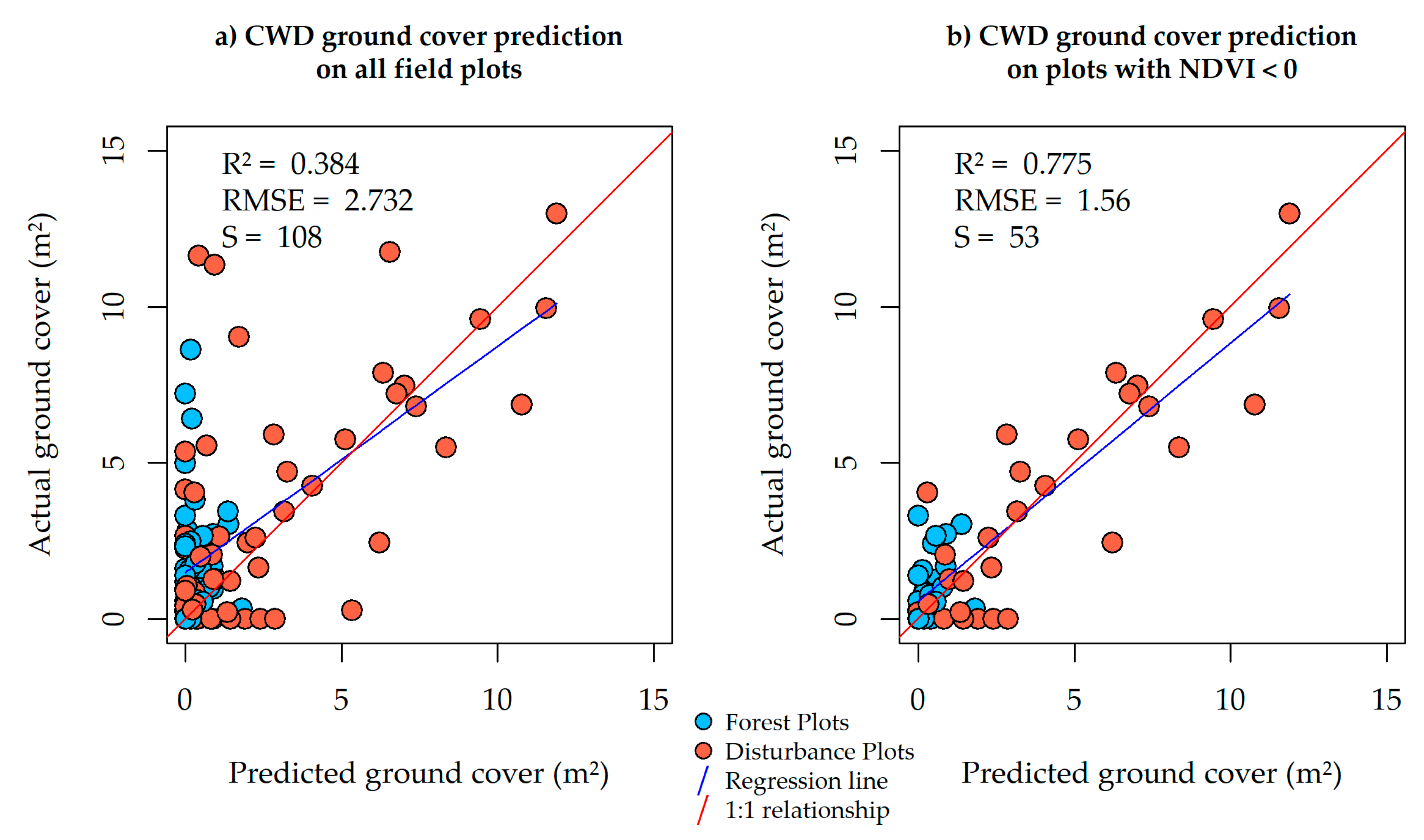
Models including aNBR placed higher than models without ML data as seen in Table 3, and the best ML-inclusive model yielded more accurate results than the best model without ML variables, with lower RMSE and higher R2 as seen in Figure 3. It is also visible between Figure 3a,c that the plots that benefited the most from the inclusion of ML variables were the plots with large amounts of CWD above the regression line; in other words, plots with underpredicted CWD volume. When analyzing our orthophotos and field photos of these plots we noticed that most of them were also affected by either closed canopy (off the seismic lines) or tall grass (on the seismic lines). Furthermore, as seen on Figure 7, the vCWD layer produced via GEOBIA is only a good estimator of CWD quantities on plots where CWD is not being occluded by closed canopy or tall grass (Figure 7b), and produces a zero-inflated independent variable on Figure 7a. These results suggest that ML variables can be valuable for CWD volume estimation, likely acting as indicators of occluded CWD quantity and consequently reducing the error on plots with occluded CWD. However, given that models without ML variables were also selected as candidates, we must conclude that there was not enough evidence to make the claim that ML substantially improved our CWD volume models.

NDVI is a much more common indicator for coarse woody debris than NBR in the literature. However, in this case aNBR was selected over aNDVI within candidate models, most likely because of the reduced ground-point frequency observed in the green ML channel, which increases the relative variance of the aNDVI values obtained at each plot. The low point density and high percentage of single returns of the green ML channel are attributed to the larger beam divergence and forward tilt for this channel which causes it to encounter more foliage than the other channels. Wet surfaces caused by rain prior to the flight mission further reduced the detection capability for the green channel. We expect that data collected on drier conditions and/or lower altitude would yield a dataset with a more complete representation of ground points especially in the green channel. In that case, aNDVI would likely be a more appropriate indicator for spectral separation on CWD than aNBR, and it is possible that aNBR would not even be present in candidate models for such a dataset. Additionally, even though individual ML channels were not considered as potential variables in model selection given that active vegetation indices were assumed to be superior variables in terms of model parsimony, future studies may consider investigating the potential of separate channels as additional information for forest classification.

It is noteworthy that Okhrimenko and Hopkinson [21] demonstrated that active vegetation indices should be derived from single return averages instead of all-return averages for more consistent values across land cover types. However, in the case of this study, the point density for single-returns was not dense enough, especially on vegetated areas. Therefore, using averages from single-returns of the ML datasets presented here would in practice defeat the intended purpose of ML in this study: providing insight onto occluded CWD. Future studies may incorporate lower-altitude ML acquisition for an increased number of single returns on all channels, enabling more stable active indices.

4.3. Two-Part Models Versus Simple Models

We considered that separating the CWD volume model into a binomial and a continuous part was beneficial due to the nature of the zero-inflated response variable. Tests comparing two-part models against simple linear models revealed that two-part models primarily reduce the overprediction of plots in the lower-left corner of actual-versus-predicted CWD volume scatterplots such as those seen in Figure 3. Consequently, two-part models consistently reduced RMSE and increased R² values in relation to simple linear models when using either cross-validation or the verification area tests. Furthermore, AICc tests would place simple models well above the ΔAICc threshold of 2 and would only select two-part models as candidates.

In our study area, the spatial distribution of wetlands seems to control much of the forest structure and consequently CWD volume. It is noteworthy that wetland-related variables were selected by all binomial models but not by any of the continuous models in Table 3. This result suggests that the presence or absence of wetlands is highly related to the presence or absence of CWD, and therefore the zero-inflation effect on our response variables. Furthermore, the presence or absence of wetlands is not a strong factor for CWD volume on plots where CWD is present, which is supported by the fact that most plots with large amounts of CWD were located on uplands. This pattern is expected on seismic line treatment efforts as well, since usually operators will be instructed to apply a larger amount of CWD on upland sites than they would on wetland sites [7]. Tests comparing single linear models to two-part linear models indicated that the former consistently overpredicted CWD quantities on wetland plots with water.

4.4. Standardized Model Coefficients

The standardized coefficients of the binomial model (Table 4) reveal that all variables substantially contribute to the prediction of this model, with vCWD being the strongest predictor. The response variable for the binomial model can be understood as the likelihood of absence of CWD. Therefore, a strong negative coefficient for vCWD is to be expected and indicates that the larger the quantities of detected CWD area, the smaller the likelihood that CWD is absent. Positive coefficients for vWater and WP show that high wetness and presence of wetlands increase likelihood of absence of CWD, as would be expected given the smaller stature of the forests in these areas. A negative coefficient for standard deviation of passive NDVI leads us to believe that NDVI-homogeneous areas are less likely to contain CWD in relation to areas with high NDVI variability, which is plausible given that during leaf-on conditions (summer) ground vegetation is widespread in the study area and sites without CWD will generally have either very high NDVI in the case of vegetated areas and very low NDVI in the case of roads and open water without much variability. Conversely, sites with CWD will have the presence of low NDVI pixels on CWD and high NDVI pixels in the surrounding ground vegetation, causing a greater variance for NDVI.

Standardized coefficients of the continuous model (Table 5) reveal that aNBR was the least important predictor. This effect is not surprising considering models without ML predictor variables were tied in terms of ΔAICc with the ML-inclusive models (Table 3). Given aNBR was selected in some candidate models we assume that, to some extent, it must contain valuable information regarding the variance of CWD volume. However, its small standardized coefficient and its absence in other candidate models suggest that it does not contain substantial information to conclude it is on the same level of importance as the other variables. We believe that the information being supplied by aNBR_sd is similar to the information being supplied by pNDVI_sd in the binomial model, namely that vegetated areas without CWD will have high aNBR without much variance, and that areas with CWD will have low aNBR pixels on CWD and high aNBR pixels on the surrounding vegetation, causing greater variance. In other words, the positive nature of the aNBR_sd coefficient shows that an increase of CWD quantities can cause higher variance in aNBR captured with ML LiDAR. Finally, we believe that aNBR is not supplying substantial information about the variance of the response variable due to noise in the intensity values given that the intensity information available in LiDAR returns of the ground surface is very likely to have been affected by environmental factors such as target roughness, reflectance and wetness, as well as attenuation due to pulses being split into multiple returns [50].

A positive coefficient for squared vCWD in the continuous model shows there is a positive relationship between predicted area of CWD according to our GEOBIA and actual CWD volume. Given a negative coefficient for CC we interpreted that gaps in the canopy may indicate larger quantities of fallen trees, whereas tightly packed canopies are unlikely to have large quantities of sound logs. We recognize that this assumption may indicate the model is less capable for heavily decayed CWD. The standardized coefficients for CHM_max at Table 5 indicate that an increase of tree size has a positive relationship with CWD volume, although it relates to a tapering curve given the negative CHM_max² coefficient.

4.5. Issues and Limitations

As discussed previously, the main sources for the underprediction of CWD volume (i.e., false negatives in the vCWD raster image) in the presented models are occlusions caused by superimposed vegetation. ML data aided in diminishing the effect of occlusion, however due to low point density in ML point clouds the benefits of these datasets were limited. It is likely that more powerful ML radiometric calibration methods will be available in the future which could enable a more direct comparison between ML intensity and object reflectance, potentially even causing dense ML point clouds to eliminate the need for image analysis altogether.

Aside from the issue of gaps in the ML data due to diminished returns at ground level, the NIR ML band also displayed a noticeable banding issue caused by variations of return intensities on each laser scan line. This effect caused some noise to be translated to our aNDVI and aNBR layers, which probably reduced the accuracy of our results presented here. There have been studies on possible solutions for banding problems [51]. However, since the vegetation indices were sampled at plot level, while averaging the values of all pixels within each plot, we considered that the effect of banding was attenuated for the purposes of answering the questions posed in our study and we decided to not perform any noise attenuation procedure on our datasets. We suggest that banding issues should be addressed in order to increase accuracies in future studies.

The main sources for overprediction of CWD volume (i.e. false positives in the vCWD raster image), observed on plots below the regression line in Figure 3 seem to be: a small quantity of occluded CWD being interpreted as a large quantity of CWD, which may be attributed to the noisy nature of the ML data; and tall neighboring trees with a lower than average CWD quantity, which highlights one disadvantage of using the CHM_max variable as an indicator for CWD volume. The presence of the canopy closure (CC) and height of tallest tree (CHM_max) variables in all candidate models might be indicating that the ML data is not providing enough information about the occluded portions of the study area, and that the height of the tallest tree within each plot as well as the percentage of occluded area are supplementing that lack of information and improving the CWD volume estimates. If the ML datasets were more comprehensive and consistent, the value of CC and CHM_max variables would likely diminish.

Aside from the sources of overprediction described above, upon close examination of the final maps presented in Figure 4 and Figure 5 we found additional sources of localized error: clear-cut edges, isolated snags and wet mud surfaces. Some shadowed edges between clear-cuts and natural forest seem to have caused overprediction of CWD, probably given that our sampling design avoided and therefore did not account for these transitions between forest and disturbances. Some isolated snags, especially on clear-cuts, caused CWD overprediction; even though in some studies snags are defined as a type of CWD in here it acts as a source of error. Additionally, extensive wet mud surfaces located on wetlands, which usually surround water bodies, are seen as highly reflective bumpy areas with low NDVI, which caused the RF classifier to overpredict CWD. These three additional sources of error present situations which were not accounted for in the training data, which reinforce the importance of having a representative sample for your application area.

Finally, we believe that our map of seismic line volume (Figure 5) should only be used as a reference for field operators and we recognize that it is likely to have lower accuracy than our map for the overall forest (Figure 6). Volume values for line segments were derived from the raster of volume in the overall area, and therefore cells positioned in an arbitrarily placed grid may be at the transition between disturbance and forest. For a better estimate of volume on seismic lines, future models should be constrained by the spatial extent of seismic lines, excluding the surrounding forest. GIS procedures could be applied to generate irregular 100 m² cells within the boundaries of seismic lines and CWD volume models could be applied to such cells for a more reliable prediction.

4.6. Future Work

We used data collected over the summer (leaf-on) to generate all intermediate products presented in this document. We believe the incorporation of spring (leaf-off) datasets as an additional resource for CWD volume estimation should increase the accuracy of predictive models especially on areas with occluded CWD. We note that upon inspection, most plots well above the regression lines on Figure 3a,c represented piles of CWD occluded by tall grass on seismic lines. On leaf-off data the CWD on these same plots should be much more distinct, since the live vegetation is less dense that time of year. Additionally, it is possible that incorporating the ML datasets into the GEOBIA workflow may increase the accuracy of the vCWD layer. Moreover, while our study focused on coarse woody debris, it is likely that similar models could be applied to estimate fine woody debris (FWD, <7 cm diameter or <1 m length) volume assuming FWD is affected by the same parameters presented in the selected models for CWD volume. The impact of a finer object of study on the accuracy of models using the presented methods is yet to be tested. Finally, it is unclear if ensemble models could perform better than single models within this context given most linear models presented here as candidate models were quite similar.

We encourage future researchers to investigate these options, to explore the utility of other explanatory variables (e.g., time since disturbance, tree-species composition, etc.), and to test the development of remotely sensed models of CWD in other forest ecosystems. Additionally, the possibility of creating accurate high-resolution (10 m GSD) CWD maps over extensive study areas may be beneficial to improve a variety of ecological models including wildlife habitat and seismic line use models.

5. Conclusions

A method for creating accurate and extensive maps of CWD volume on boreal forests was presented in this study as a novel solution using multispectral LiDAR (ML) for volume estimation of both visible and occluded CWD. Visible CWD was mapped using geographical object-based image analysis, and occluded CWD was modeled using infra-canopy normalized burn ratio. The best zero-adjusted gamma models (ZAGA) using ML data and without ML were selected with small-sample Akaike’s information criterion (AICc). Many of the variables we predicted would control CWD quantities and occlusion were selected as predictor variables in the best models, including visible CWD area, height of tallest alive trees, canopy closure, visible water area, wetland probability, passive NDVI and active NBR. The ZAGA models performed very well when tested with the reference data, both in cross-validation tests with the training samples (0.623 R², 0.224 RMSE using ML data; 0.514 R², 0.254 RMSE without ML) as well as in verification tests using independent samples from a spatially separated from the training area (0.721 R², 0.198 RMSE using ML data; 0.628 R², 0.203 RMSE without ML). The best model using ML performed better than the best model lacking ML variables. Our final CWD volume maps provide accurate, extensive, and high-resolution (10-m GSD) estimates for our study area and provide the foundation for a variety of management activities, including seismic line restoration and fire-hazard assessment.

CWD used to protect regeneration efforts on seismic lines are usually applied based on the natural range observed in the environment [7]. This natural range can be accurately mapped using the method presented here. Field operators can use extensive maps of CWD volume as guides to select areas for CWD treatment as well as for improved navigation in seismic lines. Conversely, large accumulations of CWD which can constitute a fire hazard [52] can be detected in these map products and addressed to prevent wildfires.

The methods presented here could be applied to any forested environment to generate extensive CWD volume maps which may be used for forest management as well as ecological research. Some methodological steps of our method may be improved and expanded, such as the inclusion of leaf-off data and the use of ensemble models. ML-derived vegetation indices proved to be useful in detecting CWD but could not be applied reliably to generate active NDVI due to attenuation losses in the green channel. Moreover, even though ML was helpful for modelling occluded CWD, a lack of ground returns in closed canopy areas limited the efficacy of these datasets and showcased that modelling occluded forest targets remains a technical challenge. More research is required in this context.