Article

Impacts of Change in Atmospheric CO2 Concentration on Larix gmelinii Forest Growth in Northeast China from 1950 to 2010

Key Laboratory of Sustainable Forest Ecosystem Management-Ministry of Education, School of Forestry, Northeast Forestry University, Harbin 150040, China
*
Author to whom correspondence should be addressed.
Forests 2019, 10(5), 454; https://doi.org/10.3390/f10050454
Submission received: 19 March 2019 / Revised: 11 May 2019 / Accepted: 17 May 2019 / Published: 25 May 2019
(This article belongs to the Section Forest Ecology and Management)

Abstract

:
Although CO2 fertilization on plant growth has been repeatedly modeled to be the main reason for the current changes in the terrestrial carbon sink at the global scale, there have been controversial findings on the CO2 fertilization effects on forests from tree-ring analyses. In this study, we employed conventional dendrochronological tree-ring datasets from Northeast China, to detect the effect of CO2 fertilization on Larix gmelinii growth from 1950 to 2010. Among four sites, there were two sites exhibiting a significant residual growth enhancement at a 90% confidence level after removing the size, age and climaterelated trends of tree-ring indices. In addition, we found consistency (R from 0.26 to 0.33, p < 0.1) between the high frequency CO2 fluctuation and residual growth indices at two of the four sites during the common period. A biogeochemical model was used to quantitatively predict the contribution of elevated atmospheric CO2 on accumulated residual growth enhancement. As found in the tree-ring data, 14% of the residual growth was attributed to the CO2 fertilization effect, while climate was responsible for approximately the remainding 86%.

1. Introduction

The rapid increase in CO2 concentration in the atmosphere as a greenhouse gas is thought to be responsible for the increase in earth’s surface temperature [1]. The response of forest ecosystems to elevated atmospheric CO2 concentration will affect their net uptake or loss of carbon and may, therefore, have large consequences on the global carbon cycle [2]. Numerous global-level experiments were conducted to investigate and understand how the terrestrial ecosystem carbon cycle responds to rising atmospheric CO2. Recent studies based on terrestrial carbon cycle models suggested that the strength of the terrestrial C sink was growing at the global scale, while CO2 fertilization was the predominant driver of the growth in the terrestrial C sink [3,4,5,6]. Free air CO2 enrichment (FACE) experiments [7,8,9,10] also showed considerable growth enhancement due to the CO2 fertilization effects. In spite of the wealth of global assessments and experimental evidences on CO2 fertilization on tree growth, results from tree-ring studies on the CO2 fertilization effect are controversial and still under debate [11,12,13,14,15,16,17].
It is widely held that the postindustrial rise in the concentration of CO2 in the atmosphere should have enhanced tree growth through a fertilization effect, that can be ascribed this CO2 fertilization effect on growth to the following two main mechanisms: first, direct CO2 fertilization may occur because the higher partial pressure of CO2 increases the rate of CO2 reactions with Rubisco during photosynthesis, and inhibits photorespiration [18]. Second, the increase in water-use efficiency takes place when the stomatal conductance is reduced but, at the same time, also the assimilation is kept constant or increasing, which results in an increase in the ratio of carbon gain to water loss [19]. As expected, several tree-ring studies have reported an increase in radial growth of trees with the rise of atmospheric CO2 concentration in natural forests [11,12,13]. In contrast, some studies did not find any evidence of this CO2 fertilization effect as a cause for enhanced tree growth in mid- and high-latitude forests of the northern hemisphere [15,16,17]. It may be argued that the CO2 fertilization effect on forests at high latitudes is either non-existent because of other growth-limiting conditions such as temperature and nitrogen or is too small to detect [20,21].
Here, the objective of our study is to apply tree-ring analysis approaches to detect possible effects of atmospheric CO2 fertilization on natural Larix gmelinii forests in Northeast China over the period 1950–2010. We examined the time-related trend in the residual growth after removing size-, age- and climate-related trends through conventional dendrochronological analysis. Consequently, any CO2-induced increases in productivity could be evident as an increase in the residual tree-ring width. Meanwhile, an integrated terrestrial ecosystem C-budget (InTEC) model [22], which integrates stand development with the effects of environmental conditions on growth, was used to assess the contributions of climate factors, and increased CO2 concentration on growth enhancements in stemwood from 1950 to 2010. Finally, we will directly evaluate whether the CO2 fertilization effect is significant in forest stands at high latitudes.

2. Materials and Methods
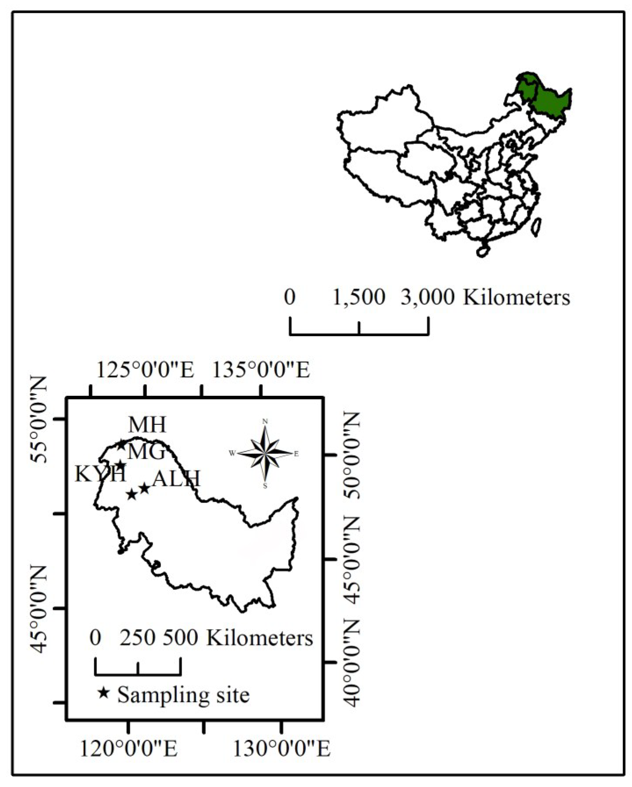
2.1. Tree-Ring Data

Increment cores of Chinese Larix gmelinii trees were collected from four sites. All sites were selected in stands with low levels of human disturbance and distributed in the main forest areas of Northeast China (Figure 1). These sites include four mature-tree sites (more than 200 years): Mohe, Heilongjiang, China (MH), Mangui, Inner Mongolia, China (MG), Alihe, Inner Mongolia, China (ALH), and Keyihe, Inner Mongolia, China (KYH). We measured annual growth increments from the pith to the outermost ring at a precision of 0.001 mm using a Velmax measuring system (sliding stage, Velmex Inc., Bloomfield, NY, USA), dating and measurement errors were further checked with COFECHA software [23]. Finally, a total of 171 cores (1 per tree) were collected, and ring-width measurements were recorded for a period extending from 1715 to 2010 (Table 1).

2.2. Tree-Ring Approach

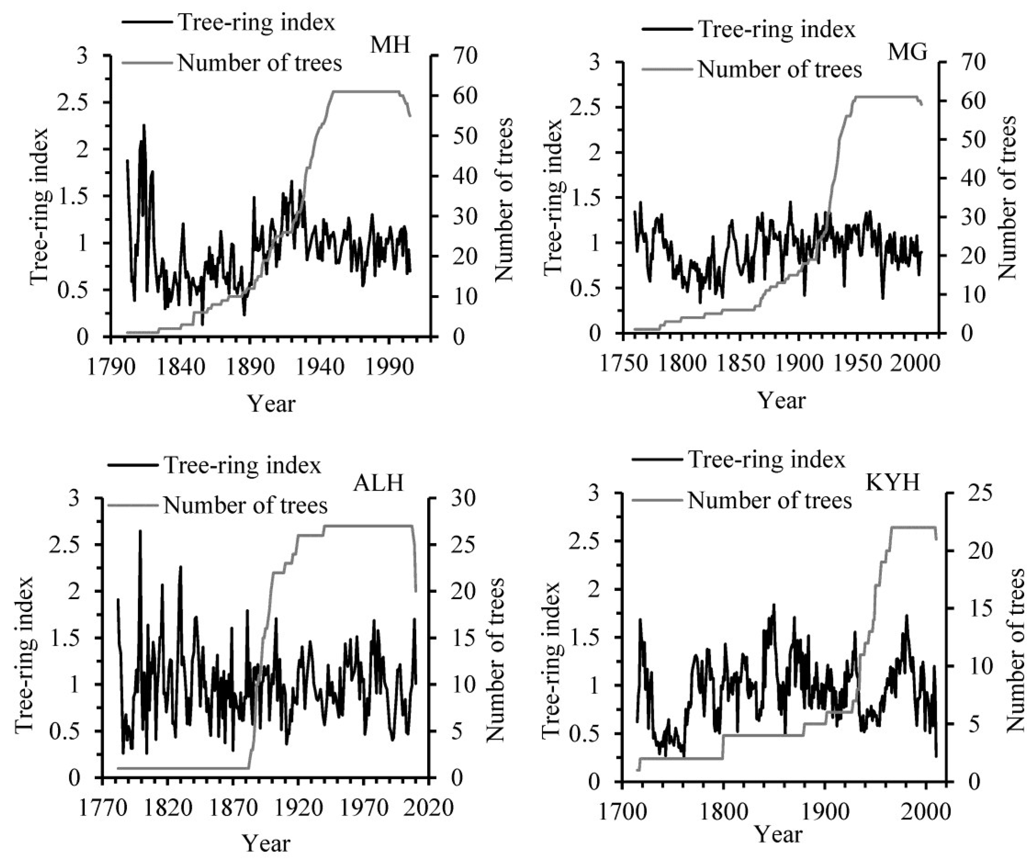
2.2.1. Chronology Development

All of the ring-width measurements were detrended using linear lines or negative exponential curves. These conservative approaches to detrending should preserve virtually all of the low-frequency variability in the tree ring series [24]. The standard (STD) chronologies were then generated for each site. All series were created by the program ARSTAN [24] (Figure 2). The statistical characteristics of the STD chronologies for each site include (Table 2): the mean index and standard deviation (Std.) of the STD chronologies; the skewness and kurtosis are included to assess the effects on the probability distribution owing to the method of standardization [25]; the mean sensitivity, which quantifies the relative change in width among consecutive years [26]; the serial correlation is used to describe the correlation of each ring width with the preceding ring width [26]; the Rbar express average correlation among trees for the common overlap period among series [26]; the expressed population signal (EPS) (Equation (1)) is used to test the chronology confidence and strength of the common signal in the chronology. We employed 0.85 as an expressed population signal (EPS) threshold value to assess the robustness, which has been widely suggested as reliable [11,12,27].
EPS = N r ¯ 1 + ( N 1 ) r ¯  
where N is the number of trees, r ¯ is the mean inter-series correlation.

2.2.2. Dendroclimatic Analysis

Our dendroclimatic analysis was conducted by using the program PRECON [28] throughout 1950–2010 for four sites. In this work, a climatic response function analysis was performed with monthly mean temperatures and total precipitation records (from June of the previous year to October of the current year) as climatic predictors, and the STD chronologies as the dependent variables. Then the predicted ring-width indices were estimated through multiple regression, after extracting the principal components of the climatic predictors that explained the greatest variation in radial growth. This includes a bootstrap method to assess statistical significance of the regression coefficients in response functions. In this work, 1000 iterations were computed to estimate the confidence intervals of regression coefficients (p < 0.05). If the confidence interval for the mean of a bootstrapped estimate of a regression coefficient does not include zero, the association between growth and that climate variable is deemed statistically significant. The final residual indices (STD residuals) could be calculated as actual indices minus predicted indices; this process means that these climatically induced variabilities have been removed from the STD tree-ring chronologies.

2.3. CO2 Fertilization Test

To test the CO2 fertilization hypothesis, we used two methods. First, a nonparametric method was implemented in this study for detecting the trend of residual indices after removing the effects of age and climatic variability from 1950–2010. If a linear trend exists, the true slope can also be estimated by a nonparametric procedure developed by Sen (1968) [29], which is closely linked to the Mann–Kendall test [30]. The Sen’s method is not much affected by outliers and can be computed with missing data. Then the residual indices (STD residuals) were tested for an increasing trend in growth over time that cannot be attributed to climate by the Sen’s method. This test is premised on the assumption that once the effects of climatic variability have been removed from the chronologies, the residual indices should exhibit an increasingly positive bias over time due to CO2 growth stimulations [14].
Second, to test the effect of CO2 fluctuation on tree growth variation, we calculated the first order difference of the raw CO2 concentration, then the linear trend was removed from the first order difference of the raw CO2 concentration. In this way, a high frequency fluctuation in CO2 concentration could be produced and correlated with interannual variations in tree growth [12]. Then, the comparisons were performed between the CO2 fluctuation time series and the STD residuals for four sites, respectively.

2.4. Description of the InTEC Model

The InTEC model is a process-based biogeochemical model that mechanistically integrates the effects of non-disturbance factors (climate variables and atmospheric CO2) and disturbance factors (disturbance and regrowth) on the long-term C and N cycles in forest ecosystems. The model includes five core processes: (a) simulation of net primary production (NPP) in a recent reference year (NPPref) using a two-leaf canopy photosynthesis model based on Farquhar’s leaf-level biochemical model [31]; (b) based on NPPref and past climate, the initial value of NPP in the starting year (NPP0) of simulation is reconstructed retrospectively through iterative adjustments of NPP0, until the simulated NPP in the reference year agree with NPPref to within ±1%; (c) the NPP of a region for each pixel in any year is calculated from the NPP0 multiplied by a factor that integrates the effects of non-disturbance factors (ϕNPP) and forest stand age (FNPP(i)) (Equation (2)). In the InTEC model, NPP-age relationships are replaced by normalized productivity (FNPP) curves (Equation (3)) [32]. The curves are obtained by dividing NPP at a given age by their maximum NPP value in their forest life cycle with values ranging from 0 to 1. These relationships are used to simulate forest regrowth after disturbance and changes in the different C components; (d) a three-dimensional distributed hydrological model is used to simulate soil moisture and temperature [33]; and (e) a modified CENTURY model [34] and the net N mineralization model [35] are employed to simulate soil C and N cycles.
N P P ( i ) = N P P 0 × N P P ( i ) × F N P P ( i )
F N P P ( i ) = N P P ( i ) / N P P m a x
where NPP(i) represents the NPP at age i, NPPmax represents a maximum of NPP.

2.4.1. Model Inputs

In order to drive the InTEC model, several spatial datasets were created in this study, including monthly mean temperature, water vapor pressure, and total precipitation, which were collected from the UK Climate Research Unit [36], and monthly solar irradiance data was from the US National Center for Atmospheric Research [37]. A map of stand age in 2010 [38] and a forest type map in 2006 [39] were created from forest inventory data in this study. A reference NPP map in 2003 was producted by using the boreal ecosystem productivity simulators (BEPS) [40]. The annual atmospheric CO2 concentrations from 1950 to 2010 were taken from the dataset obtained at the Mauna Loa Observatory (20° N, 156° W) [41]. A maximum leaf area index (LAI) map was produced in 2003 by Deng et al. [42] using SPOT-VEGETATION data. The physical properties of the soil used in the InTEC, including the field capacity of soil water, wilting point, soil depth, and the fractions of clay, silt, and sand, were included. Field capacity and wilting point were derived from the International Geosphere-Biosphere Programme, Global Gridded Surfaces of Selected Soil Characteristics [43]. Soil depth was derived from the global soil texture dataset from Oak Ridge National Laboratory Distributed Active Archive Center, Tennessee, U.S. [44]. The fractions of clay, silt, and sand were obtained from the Harmonized World Soil Database (HWSD) constructed by the Food and Agriculture Organization of the United Nations (FAO) and the International Institute [45].All of these spatial datasets were employed in the UTM WGS-84 coordinate system and interpolated to 1 km resolution. Detailed descriptions of datasets were reported elsewhere [46,47].

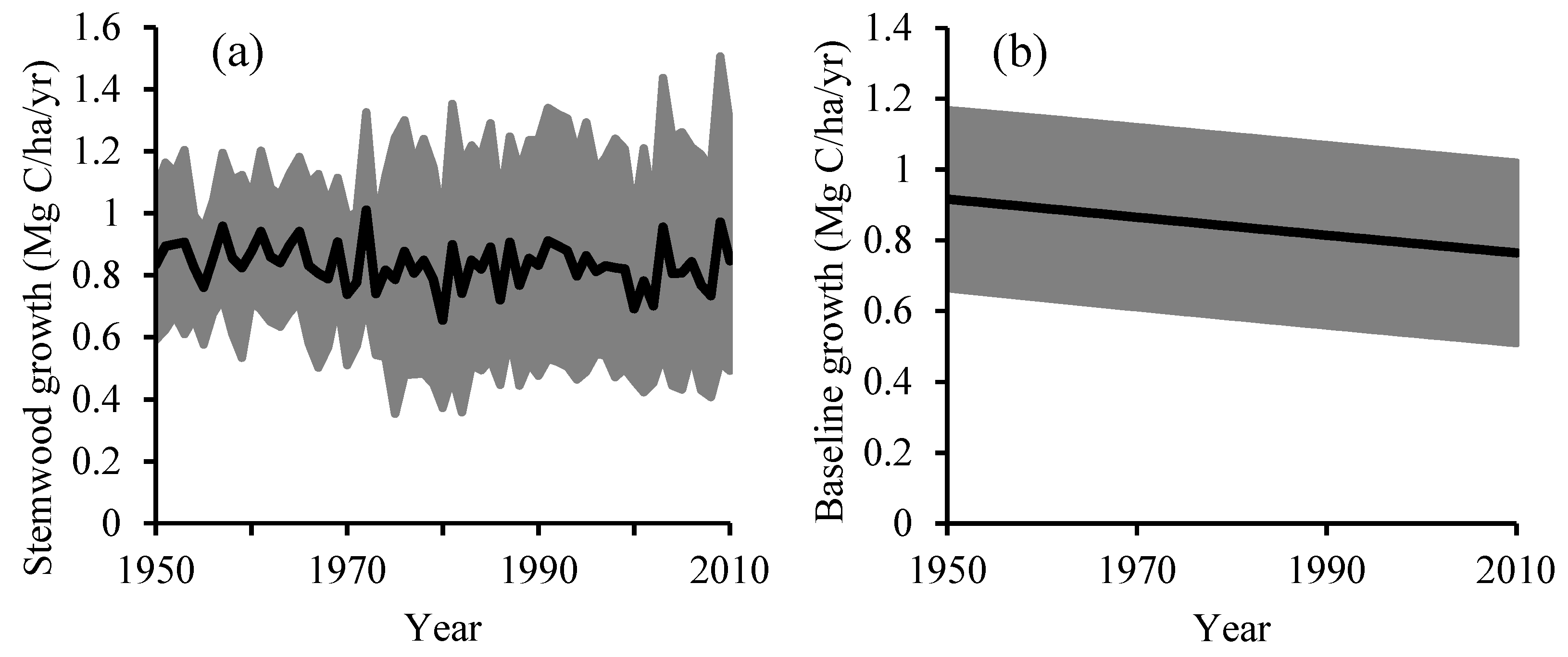
2.4.2. Stemwood Biomass Growth

We used InTEC to estimate the stemwood biomass growth (G_SW) of Larix gmelinii forests at four sites from 1950–2010. In this study, we assumed that stemwood growth consists of 31% of NPP in InTEC simulations [48].

2.4.3. Baseline and Residual Stemwood Biomass Growth

The yield table for Larix gmelinii of Heilongjiang Province, China was developed by the Forest Survey Scheme Designing Institute in 2010. It was collected to provide information on the stand development, such as mean age, stand density (S), volume (V) and mean volume growth (Vg). The age ranges in the yield table are 0–150, and five-year intervals were used in the yield tables. Using this information, the baseline stemwood growth (B_SW) can be calculated based on the stand biomass equation.
We used Equation (4) to calculate the B_SW for Larix gmelinii forests at different ages by combining stand mean volume growth and age information in the yield table. The regression coefficients in Equation (4) were taken from Dong (2015) [49]. The age response of B_SW (B_SW(age)) was then fitted using the Weibull distribution function as Equation (5) [32] (Figure 3). Finally, the residual stemwood biomass growth (R_SW), which includes only the total signal of external forcings (e.g., climate, CO2, and N) was determined as the difference between G_SW and B_SW.
B_SW = exp ( a + b × log V g ) × C s
B_SW ( A ) = a 1 ( 1 + a 2 ( A a 3 ) a 4 1 exp ( A a 3 ) )
where log denotes natural logarithm; a and b are regression coefficients; B_SW is baseline stemwood biomass growth (Mg/ha/yr); Vg is mean stand volume growth (m3/ha/yr), which is available in the yield table; A represents stand age (years); a1, a2, a3, and a4 are fitted parameters that were listed in Table 3. We set the C content in stemwood as 0.47 in this study [50].
In this study, we did not integrate the age and size effects on stemwood growth from the observed tree-ring index into the InTEC model because of lacked of sufficient information to establish the NPP-age relationships for Larix gmelinii at these sites. Although, the B_SW-age relationship we established by using the yield table could represent the long-term average state of age response of B_SW at these sites. In addition, the stemwood growth component in the NPP-age relationship which integrated in the InTEC model was also calculated by using the same yield table and biomass equation as in this study [48], so that the age effect could be completely removed from simulated stemwood growth.

2.4.4. The Partitioning Approach to Attribute Growth Variation to Various Factors

To examine the relative individual effects on growth of climate factors and CO2 concentration on stemwood growth enhancement, we designed a series of modeling experiments by setting one factor in question constant at a time while using realistic historical values for all other factors in the simulation. For example, to investigate the effect of CO2 on growth, we first set CO2 to be a constant as the average over the 1901–1910 period, while the historical values of other factors were used in the simulation. We then detect the CO2 effect as the difference between the full historical simulation and the constant CO2 simulation.

3. Results

Our climate-growth response function analysis showed that no clear common patterns were observed in the relationships between climate and radial growth across the four mature-tree sites (Figure 4). The high temperature during the growing season was generally unfavorable for tree growth at these sites, especially in June and July of the current year. The growing season precipitation was positively correlated with the tree growth, while negative correlations could be found in the winter months (from December of the previous year to February of the current year). Additionally, 58%, 63%, 52% and 56% of the variance in the raw growth indices of MH, MG, ALH, and KYH was explained by mean temperature and precipitation for the period 1950–2010. Based on these responses to climate variations, the predicted growth indices could be producted for each site; then we calculated residual indices by subtracting predicted from raw tree-ring indices.
Among the four sites, ALH and KYH exhibited a positive trend in their STD residuals at a 90% and 95% confidence level, respectively (Figure 5a,b), but the other two sites (MH and MG) did not have a significant positive trend in their residuals (Figure 5c,d).
We then compared the residual indices with high frequency CO2 interannual fluctuation (the linear trend was removed from the first order annual difference of the raw CO2 concentration) (Figure 6). Two sites showing a statistically significant positive correlation between the CO2 fluctuation and residual indices (Pearson’s correlation coefficient (R) from 0.26 to 0.33, p < 0.1), except for MH (R = −0.01, p > 0.05) and MG sites (R = 0.08, p > 0.05), which also failed to detect a significant upward trend in their residual indices.
The relationship between stand age and baseline stemwood growth (B_SW) for Larix gmelinii was produced by using yield tables (Figure 3). The B_SW increased with stand age initially, reached a peak, then declined slowly at an approximately constant rate. For all sites, the curve presented a trend of slow decrease from 1950 to 2010 (Figure 7b), and it indicated that the stand age had a negative effect on stemwood growth since 1950.
We removed the age effect from stemwood growth (G_SW) (Figure 7a) to calculate the residual stemwood growth (R_SW), and then we compared the R_SWs with the STD chronologies for each site, respectively. The R_SWs agreed well with those STD chronologies with a correlation coefficient from 0.27 to 0.51 (p < 0.05) as shown in Figure 8. Through these site-level comparisons, there were reasons to believe that InTEC was a reliable model to link historical climate data and reconstruct the interannual variability of tree growth that was induced by external factors.
The contributions of climate and CO2 on R_SW were partitioned using the approach described in the methods section. Overall, 86% of accumulated R_SW was mainly attributed to climate (Figure 9a). The CO2 concentration increased from 346 ppmv in 1950 to 387 ppmv in 2010. The elevated CO2 contributed to accumulated R_SW by 14%. We also further separated the total climate effect into those from temperature, precipitation, radiation, and water vapor pressure (Figure 9b). Among the four climate factors, temperature was the dominating factor contributing 73% to the changes in the accumulated R_SW. The second was precipitation, at 20%, followed by water vapor pressure at 4% and radiation at 3%.

4. Discussion

Trees from cold environments may show either positive or negative growth responses to warming depending on both inherent acclimation potential and other potentially limiting factors [51]. Our results indicate that high temperature generally has a negative effect on the growth of Larix gmelinii at four sites, particularly in June or July (Figure 4). This result agrees with similar studies about coniferous trees in northern China [12,52]. High temperature can cause an increase in transpiration, evaporation, moisture loss, and the internal nutrient consumption of the trees, and since dark respiration is a temperature-dependent process, warmer temperatures increase the respiration rates of plants, which results in decreases in the accumulation of carbohydrate content in plants, and consequently limits growth [53].
In our tree-ring analysis, two sites exhibited evidence of residual indices (after removing the effects of age and climatic variability) to increase in response to increasing CO2 (Figure 5c,d). These results indicate that tree growth has a “CO2 acclimation” response to CO2 enhancement [18,19,20]. We failed to detect a statistically significant positive trend in the residual indices at the MH and MG sites (Figure 5a,b). These two sites are located at higher latitudes, and the CO2 fertilization effect may be severely limited by lower temperatures (annual mean temperature was −5.1 °C for MH site and −6.0 °C for MG site, respectively) there. Many studies reported that low temperature in some cases might impair Rubisco activity and diminish the positive influence of higher CO2 on photosynthesis [54,55]. In addition, lower temperature makes the growing season shorter, giving little opportunity for trees to allocate carbon to the cambial production of stem tissue even if limited growth enhancement has occurred [56].
Some consistency was found between the time series of CO2 high-frequency fluctuation and residual indices at two sites (R from 0.26 to 0.33, p < 0.05) (Figure 6c,d). This result indicate that interannual variations in tree growth was linked to the high-frequency fluctuation of CO2 concentration. Our result was similar to that of Chen et al. [12], who reported that there was a significant correlation between CO2 high-frequency fluctuation and tree-ring indices in Pinus tabuliformis in the northeast of China over 1950–2010. These results reinforce our findings that conventional dendrochronological techniques can detect the effect of CO2 fluctuations on yearly tree growth in coniferous forests.
It is not easy to quantitatively separate the CO2 fertilization effect on tree growth from those of external environment factors. The InTEC model can not only capture key ecosystem processes but also describe interactions of terrestrial ecosystems with environmental forcing factors. Also, systematic tree growth-age relationships were integrated into the InTEC model, making it possible to remove the influences of the intrinsic age factors [57]. Our model results indicate that 14% of accumulated R_SW can be attributed to atmospheric CO2 increase (Figure 9a). Although increased CO2 contributed only a small fraction to the overall growth enhancement, it may be important to fully explain the carbon balance in mid to high northern latitude forests.
The CO2 fertilization effects reported were not uniform across the forest sites investigated [11,12,13,14,15,16]. Stand characteristics might be partly responsible for this cross-site variability [7,58]. Our results agree with most reports for Canadian, American and Chinese forests in terms of tree-ring analysis or terrestrial carbon model [12,57,59], and these results collectively provided clear evidence for greater efficiency of CO2 uptake in plants from mid and high altitudes of the northern hemisphere [60,61]. Our results also support another view that the CO2 fertilization would be more evident in the environments with annual precipitation between 300 mm and 500 mm [62,63].
Based on the increasing CO2 fertilization evidences from many short-term CO2-enriched experiments and dendrochronological tree-ring studies, we speculated the failures of some studies [15,16,17] in detecting the CO2 fertilization effect to be due to the following possible reasons: (1) temperature-limiting and N-limiting regions could preclude a direct CO2 growth response by trees [20]; (2) many biased sampling of trees could also produce spurious trends in growth rates (i.e., slow-grower survivorship bias and big-tree selection bias), consequently, a small increase in biomass increment due to the CO2 fertilization effect may be diminished [64]; and (3) carbon partitioning and growth within a plant that is species-specific [20].
Our results also point to weaknesses and additional work in the future: First, the NPP allocation coefficient to stemwood growth was set to a constant for Larix gmelinii based on the calculation results by using forest inventory data and yield tables [48]. However, the allocation coefficient varies with forest types, stand age, and environment. Unfortunately, due to lack of enough information, we could not calculate NPP allocation coefficients for each site. The use of forest inventory allowed us to check whether the allocation coefficients was reasonable for Larix gmelinii. We observed a 17% underestimate in simulated stemwood growth from InTEC compared with the forest inventory data for the period 2000–2005. Clearly, significant improvements can still be made in the relative allocation to stemwood component once more data become available. Second, since it is difficult to exclude the impact of atmospheric deposition of N on tree-ring growth; we could not be sure that the residual growth in the tree ring data was entirely due to the CO2 fertilization effect. Although many studies suggest the N deposition effect was small with a very weak trend over the study period [65,66,67], these estimates could be refined with additional N data. Third, due to limited availability of high quality tree ring data, we have access to data only for four sites. Although we have confidence in the detected CO2 fertilization signals, data at more sites are needed to assess the latitudinal gradient of these signals.

5. Conclusions

In this study, we employed a series of approaches for detecting the effect of CO2 fertilization on Larix gmelinii tree growth in Northeast China from 1950–2010. We conclude from tree-ring analysis that elevated atmospheric CO2 had a positive effect on tree growth. Meanwhile, the change in annual tree growth was found to be significantly correlated to CO2 interannual fluctuations. These results indicate that the CO2 fluctuations influence the high-frequency growth variability, but not necessarily the overall tree growth. Our InTEC modeling results also suggest that the growth change over 61 years cannot be explained by climate alone, 14% of accumulated R_SW can be attributed to CO2 increase, while the remaining approximately 86% can be attributed to climate.

Author Contributions

B.W., M.L. and W.F. conceived of the study and designed the methodology; B.W., Y.Y. and W.J. collected the data; B.W. and Y.Y. analyzed the data; B.W. and M.L. led the writing of the manuscript. All authors contributed substantially to the drafts and provided final approval for publication.

Funding

This research was funded by the National Key Research and Development Program of China (2017YFD0600902-5 and 2017YFD0600404-2) and the National Natural Science Foundation of China (31870621).

Acknowledgments

We appreciate Xiaochun Wang and Weiwei Jia for providing the tree-ring data; models in support of this article were from the research collaboration with Jingming Chen at the University of Toronto. This work was supported by the National Key Research and Development Program of China (2017YFD0600902-5 and 2017YFD0600404-2) and the National Natural Science Foundation of China (31870621).

Conflicts of Interest

The authors declare no conflict of interest.

References

  1. IPCC. Climate Change 2007: Synthesis Report. 2007. Available online: http://www.ipcc.ch/ (accessed on 5 January 2019).
  2. Bonan, G.B. Forests and climate change: Forcings, feedbacks, and the climate benefits of forests. Science 2008, 320, 1444–1449. [Google Scholar] [CrossRef]
  3. Piao, S.; Sitch, S.; Ciais, P.; Friedlingstein, P.; Peylin, P.; Wang, X.; Ahlström, A.; Anav, A.; Canadell, J.G.; Cong, N.; et al. Evaluation of terrestrial carbon cycle models for their response to climate variability and to CO2 trends. Glob. Chang. Boil. 2013, 19, 2117–2132. [Google Scholar] [CrossRef] [PubMed]
  4. Smith, W.K.; Reed, S.C.; Cleveland, C.C.; Ballantyne, A.P.; Anderegg, W.R.; Wieder, W.R.; Liu, Y.Y.; Running, S.W. Large divergence of satellite and Earth system model estimates of global terrestrial CO2 fertilization. Nat. Clim. Chang. 2015, 6, 306–310. [Google Scholar] [CrossRef]
  5. Liu, S.Q.; Zhuang, Q.L.; Chen, M.; Gu, L.H. Quantifying spatially and temporally explicit CO2 fertilization effects on global terrestrial ecosystem carbon dynamics. Ecosphere 2016, 7, e01391. [Google Scholar] [CrossRef]
  6. Huntzinger, D.N.; Michalak, A.M.; Schwalm, C.; Ciais, P.; King, A.W.; Fang, Y.; Schaefer, K.; Wei, Y.; Cook, R.B.; Fisher, J.B.; et al. Uncertainty in the response of terrestrial carbon sink to environmental drivers undermines carbon-climate feedback predictions. Sci. Rep. 2017, 7, 1–8. [Google Scholar] [CrossRef] [PubMed]
  7. Norby, R.J.; DeLucia, E.H.; Gielen, B.; Calfapietra, C.; Giardina, C.P.; King, J.S.; Ledford, J.; McCarthy, H.R.; Moore, D.J.; Ceulemans, R.; et al. Forest response to elevated CO2 is conserved across a broad range of productivity. Proc. Natl. Acad. Sci. USA 2005, 102, 18052–18056. [Google Scholar] [CrossRef] [PubMed]
  8. Körner, C.H.; Morgan, J.; Norby, R. CO2 fertilization: When, where, howmuch? In Terrestrial Ecosystems in a Changing World Series: Global Change—The IGBP Series; Canadell, J.G., Pataki, D., Pitelka, L., Eds.; Springer: Berlin, Germany, 2007; pp. 9–21. [Google Scholar]
  9. Hickler, T.; Smith, B.; Prentice, I.C.; Mjöfors, K.; Miller, P.; Arneth, A.; Sykes, M.T. CO2 fertilization in temperate FACE experiments not representative of boreal and tropical forests. Glob. Chang. Biol. 2008, 14, 1531–1542. [Google Scholar] [CrossRef]
  10. Girardin, M.P.; Bernier, P.Y.; Raulier, F.; Tardif, J.C.; Conciatori, F.; Guo, X.J. Testing for a CO2, fertilization effect on growth of canadian boreal forests. J. Geophys. Res. Biogeosci. 2015, 116, G01012. [Google Scholar]
  11. Wang, G.G.; Chhin, S.; Bauerle, W. Effect of natural atmospheric CO2 fertilization suggested by open-grown white spruce in a dry environment. Glob. Chang. Boil. 2006, 11, 1–10. [Google Scholar]
  12. Chen, Z.; Zhang, X.; He, X.; Davi, N.K.; Li, L.; Bai, X. Response of radial growth to warming and CO2, enrichment in southern Northeast China: A case of Pinus tabulaeformis. Clim. Chang. 2015, 130, 559–571. [Google Scholar] [CrossRef]
  13. Huang, J.G.; Zhang, Q.B. Tree-rings and climate for the last 680 years in Wulan area of northeastern Qinghai-Tibetan Plateau. Clim. Chang. 2007, 80, 369–377. [Google Scholar] [CrossRef]
  14. Gedalof, Z.; Berg, A.A. Tree ring evidence for limited direct CO2 fertilization of forests over the 20th century. Glob. Biogeochem. Cycles 2010, 24, GB3027. [Google Scholar] [CrossRef]
  15. Schweingruber, F.H.; Briffa, K.R.; Jones, P.D. A tree-ring densitometric transect from Alaska to Labrador. Comparisons of ring-width and maximum-latewood-density chronologies in the conifer belt of northern North America. Int. J. Biometeorol. 1993, 37, 151–169. [Google Scholar] [CrossRef]
  16. Mäkinen, H.; Nöjd, P.; Mielikäinen, K. Climatic signals in annual growth variation of Norway spruce (Picea abies) along a transect from central Finland to the Arctic timberline. Can. J. Res. 2000, 30, 769–777. [Google Scholar] [CrossRef]
  17. Girardin, M.P.; Bouriaud, O.; Hogg, E.H.; Kurz, W.; Zimmermann, N.E.; Metsaranta, J.M.; de Jong, R.; Frank, D.C.; Esper, J.; Büntgen, U.; et al. No growth stimulation of Canada’s boreal forest under half-century of combined warming and CO2 fertilization. Proc. Natl. Acad. Sci. USA 2016, 113, E8406–E8414. [Google Scholar] [CrossRef] [PubMed]
  18. Bazzaz, F.A. The response of natural systems to the rising global CO2 levels. Annu. Rev. Ecol. Syst. 1990, 21, 167–196. [Google Scholar] [CrossRef]
  19. Field, C.B.; Jackson, R.B.; Mooney, H.A. Stomatal responses to increased CO2: Implications from the plant to the global scale. Plant Cell Environ. 1995, 18, 1214–1225. [Google Scholar] [CrossRef]
  20. Huang, J.G.; Bergeron, Y.; Denneler, B.; Berninger, F.; Tardif, J. Response of Forest Trees to Increased Atmospheric CO2. Crit. Rev. Plant Sci. 2007, 26, 265–283. [Google Scholar] [CrossRef]
  21. Jacoby, G.C.; D’Arrigo, R.D. Tree-rings, carbon dioxide and climatic change. Proc. Natl. Acad. Sci. USA 1997, 94, 8350–8353. [Google Scholar] [CrossRef]
  22. Chen, W.J.; Chen, J.M.; Cihlar, J. An integrated terrestrial carbon-budget model based on changes indisturbance, climate, and atmospheric chemistry. Ecol. Model. 2000, 135, 55–79. [Google Scholar] [CrossRef]
  23. Holmes, R.L. Computer-assisted quality control in tree-ring dating and measurement. Tree-Ring Bull. 1983, 43, 69–78. [Google Scholar]
  24. Cook, E.R. A Time Series Approach to Tree-Ring Standardization. Ph.D. Thesis, University of Arizona, Tucson, AZ, USA, 1985. [Google Scholar]
  25. Ahmed, M.; Wahab, M.; Khan, N.; Zafar, M.U.; Palmer, J. Tree-ring chronologies from upper indus basin of Karakorum Range, Pakistan. Pak. J. Bot. 2010, 42, 295–307. [Google Scholar]
  26. Cook, E.R.; Buckley, B.M.; D’Arrigo, R.D.; Peterson, M.J. Warm-season temperature since 1600 AD. Reconstruction from Tasmanian tree-rings and their relationship to large scale sea surface temperature anomalies. Clim. Dyn. 2000, 16, 79–91. [Google Scholar] [CrossRef]
  27. Wigley, T.; Briffa, K.R.; Jones, P.D. On the average value of correlated time series, with applications in dendroclimatology and hydrometeorology. J. Clim. Appl. Meteorol. 1984, 23, 201–213. [Google Scholar] [CrossRef]
  28. Fritts, H.C.; Vaganov, E.A.; Sviderskaya, I.V.; Shashkin, A.V. Climatic variation and tree-ring structure in conifers: Empirical and mechanistic models of tree-ring width, number of cells, cellsize, cell-wall thickness and wood density. Clim. Res. 1991, 1, 97–116. [Google Scholar] [CrossRef]
  29. Sen, P.K. Estimates of the regression coefficient based on Kendall’s tau. J. Am. Stat. Assoc. 1968, 63, 1379–1389. [Google Scholar] [CrossRef]
  30. Gilbert, R.O. Statistical Methods for Environmental Pollution Monitoring; Van Nostrand Reinhold: New York, NY, USA, 1987. [Google Scholar]
  31. Farquhar, G.D.; Caemmerer, S.; Berry, J.A. A biochemical model of photosynthetic CO2 assimilationin leaves of C3 species. Planta 1980, 149, 78–90. [Google Scholar] [CrossRef] [PubMed]
  32. Chen, J.M.; Ju, W.; Cihlar, J.; Price, D.; Liu, J.; Chen, W.; Pan, J.; Black, A.; Barr, A. Spatial distribution of carbon sources and sinks in Canada’s forests. Tellus Ser. B 2003, 55, 622–641. [Google Scholar]
  33. Ju, W.; Chen, J.M. Distribution of soil carbon stocks in Canada’sforests and wetland simulated based on drainage class, topography and remote sensing. Hydrol. Process. 2005, 19, 77–94. [Google Scholar] [CrossRef]
  34. Parton, W.J.; Schimel, D.S.; Cole, C.V.; Ojima, D.S. Analysis of factors controlling soil organic matterlevels in the Great Plains grasslands. Soil Sci. Soc. Am. J. 1987, 51, 1173–1179. [Google Scholar] [CrossRef]
  35. Townsend, A.R.; Braswell, B.H.; Holland, E.A.; Penner, J.E. Spatial and temporal patterns in potential terrestrial carbon storage resulting from deposition of fossil fuel derived nitrogen. Ecol. Appl. 1996, 6, 806–814. [Google Scholar] [CrossRef]
  36. Climatic Research Unit. Available online: http://www.cru.uea.ac.uk/cru/data/ (accessed on 9 January 2019).
  37. Earth System Research Laboratory. Available online: https://www.esrl.noaa.gov/ (accessed on 9 January 2019).
  38. FRSOC. Forest Resources Statistics of China (2009–2014); Department of Forest Resources Management State Forestry Administration: Beijing, China, 2016.
  39. Zhang, X.; Sun, S.; Yong, S.; Zhou, Z.; Wang, R. Vegetation Map of the People’s Republic of China; Geography Press: Beijing, China, 2007. [Google Scholar]
  40. Liu, J.; Chen, J.M.; Cihlar, J.; Park, W.M. A Process-Based Boreal Ecosystem Productivity Simulator Using Remote Sensing Inputs. Remote Sens. Environ. 1997, 62, 158–175. [Google Scholar] [CrossRef]
  41. Carbon Dioxide Information Analysis Center (CDIAC). Available online: http://cdiac.esd.ornl.gov/ftp/trends/CO2/maunaloa.CO2 (accessed on 12 January 2019).
  42. Deng, F.; Chen, J.M.; Plummer, S.; Chen, M.; Pisek, J. Algorithm for global leaf area index retrieval using satellite imagery. IEEE Trans. Geosci. Remote Sens. 2006, 44, 2219–2229. [Google Scholar] [CrossRef] [Green Version]
  43. IGBP-DIS. Available online: http://daac.ornl.gov/cgi-bin/dsviewer.pl?ds_id=569 (accessed on 12 January 2019).
  44. ORNL. Available online: https://www.ornl.gov/ (accessed on 12 January 2019).
  45. IIASA. Available online: http://daac.ornl.gov/SOILS/guides/HWSD.html (accessed on 12 January 2019).
  46. Wang, B.; Li, M.; Fan, W.; Zhang, F.M. Quantitative simulation of C budgets in a forest in Heilongjiang province, China. iForest 2017, 10, 128–135. [Google Scholar] [CrossRef] [Green Version]
  47. Wang, B.; Li, M.; Fan, W.; Yu, Y.; Chen, J. Relationship between net primary productivity and forest stand age under different site conditions and its implications for regional carbon cycle study. Forests 2018, 5, 1. [Google Scholar] [CrossRef]
  48. Yu, Y.; Chen, J.M.; Yang, X.; Fan, W.; Li, M.; He, L. Influence of site index on the relationship between forest net primary productivity and stand age. PLoS ONE 2017, 12, e0177084. [Google Scholar] [CrossRef]
  49. Dong, L.H.; Zhang, L.J.; Li, F.R. A compatible system of biomass equations for three conifer species in Northeast, China. Ecol. Manag. 2014, 329, 306–317. [Google Scholar] [CrossRef]
  50. Yu, Y.; Fan, W.Y.; Li, M.Z. Forest carbon rates at different scales in Northeast China forest area. Chin. J. Appl. Ecol. 2012, 23, 341–346. [Google Scholar]
  51. Way, D.A.; Oren, R. Differential responses to changes in growth temperature between trees from different functional groups and biomes: A review and synthesis of data. Tree Physiol. Rev. 2010, 30, 669–688. [Google Scholar] [CrossRef]
  52. Wang, X.C.; Zhang, Y.D.; Mcrae, D.J. Spatial and age-dependent tree-ring growth responses of Larix gmelinii to climate in northeastern China. Trees 2009, 23, 875–885. [Google Scholar] [CrossRef]
  53. Rolland, C. Long term changes in the radial growth of the mountain pine (Pinus uncinata) in the French Alps as influenced by climate. Dendrochronologia 1996, 14, 255–262. [Google Scholar]
  54. Sage, R.F.; Kubien, D.S. The temperature response of C3 and C4 photosynthesis. Plant Cell Environ. 2007, 30, 1086–1106. [Google Scholar] [CrossRef]
  55. Hendrickson, L.; Ball, M.C.; Wood, J.T.; Chow, W.S.; Furbank, R.T. Low temperature effects on photosynthesis and growth of grapevine. Plant Cell Environ. 2010, 27, 795–809. [Google Scholar] [CrossRef]
  56. Lavigne, M.B. Stem growth and respiration of young balsam fir trees in thinned and unthinned stands. Can. J. For. Res. 1988, 18, 483–489. [Google Scholar] [CrossRef]
  57. Wu, C.; Hember, R.A.; Chen, J.M.; Kurz, W.A.; Price, D.T.; Boisvenue, C.; Gonsamo, A.; Ju, W. Accelerating Forest Growth Enhancement due to Climate and Atmospheric Changes in British Colombia, Canada over 1956–2001. Sci. Rep. 2014, 4, 4461. [Google Scholar] [CrossRef] [PubMed]
  58. Canadell, J.G.; Kirschbaum, M.U.; Kurz, W.A.; Sanz, M.J.; Schlamadinger, B.; Yamagata, Y. Factoring out natural and indirect human effects on terrestrial carbon sources and sinks. Environ. Sci. Policy 2007, 10, 370–384. [Google Scholar] [CrossRef]
  59. Pan, Y.; Birdsey, R.; Hom, J.; McCullough, K. Separating effects of changes in atmospheric composition, climate, and land-use on carbon sequestration of U.S. mid-Atlantic temperate forests. Ecol. Manag. 2009, 259, 151–164. [Google Scholar] [CrossRef]
  60. Kӧrner, C.; Farquhar, G.D.; Wong, S.C. Carbon isotope discrimination by plants follows latitudinal and altitudinal trends. Oecologia 1991, 99, 343–351. [Google Scholar] [CrossRef]
  61. Handa, I.T.; Kӧrner, C.; Hättenschwiler, S. A test of the tree-line carbon limitation hypothesis by in situ CO2 enrichment and defoliation. Ecology 2005, 86, 1288–1300. [Google Scholar] [CrossRef]
  62. Morgan, J.A.; Pataki, D.E.; Körner, C.; Clark, H.; Del Grosso, S.J.; Grünzweig, J.M.; Knapp, A.K.; Mosier, A.R.; Newton, P.C.D.; Niklaus, P.A.; et al. Water relations in grassland and desert ecosystems exposed to elevated atmospheric CO2. Oecologia 2004, 140, 11–25. [Google Scholar] [CrossRef]
  63. Nowak, R.S.; Ellsworth, D.S.; Smith, S.D. Functional responses of plants to elevated atmospheric CO2—Do photosynthetic and productivity data from FACE experiments support early predictions? New Phytol. 2004, 162, 253–280. [Google Scholar] [CrossRef]
  64. Brienen, R.J.; Gloor, W.E.; Zuidema, P.A. Detecting evidence for CO2 fertilization from tree ring studies: The potential role of sampling biases. Glob. Biogeochem. Cycles 2012, 26, GB1025. [Google Scholar] [CrossRef]
  65. Miller, P.M.; Eddleman, L.E.; Miller, J.M. The response of juvenile and small adult western juniper (Juniperus occidentalis) to nitrate and ammonium fertilization. Can. J. Bot. 1991, 69, 2344–2352. [Google Scholar] [CrossRef]
  66. Thomas, R.; Canham, C.; Weathers, K.; Goodale, C. Increased tree carbon storage in response to nitrogen deposition in the US. Nat. Geosci. 2010, 3, 13–17. [Google Scholar] [CrossRef]
  67. Solberg, S.; Dobbertin, M.; Reinds, G.J.; Lange, H.; Andreassen, K.; Fernandez, P.G.; Hildingsson, A.; de Vries, W. Analyses of the impact of changes in atmospheric deposition and climate on forest growth in European monitoring plots: A stand growth approach. For. Ecol. Manag. 2009, 258, 1735–1750. [Google Scholar] [CrossRef]
Figure 1. Locations of the sampling sites in Northeast China. Abbreviations for our sampling sites are MH (Mohe), MG (Mangui), ALH (Alihe) and KYH (Keyihe).
Forests 10 00454 g001
Figure 2. The standard (STD) chronologies and the number of trees for each site.
Forests 10 00454 g002
Figure 3. Variations of baseline stemwood growth with age for Larix gmelinii. Dots represent steemwood biomass growth calculated by yield tables; error bars represent standard deviation.
Forests 10 00454 g003
Figure 4. Correlation coefficients between the standard chronologies and total precipitation (■) and mean temperature (□) from June in the previous year to October in the current year for four sites over the period 1950–2010. The * denotes months with significant response function coefficients determined from the bootstrapped response model.
Forests 10 00454 g004
Figure 5. Raw growth indices (gray line), predicted growth indices (black dash line), and residual growth indices (black line), with Sen’s regression line (red line) superimposed for four sites; Q is Sen’s slope and B is a constant.
Forests 10 00454 g005
Figure 6. Comparison of the tree-ring residual indices and CO2 interannual fluctuation (the first order annual difference of the CO2 concentration) for four sites during the common period.
Forests 10 00454 g006
Figure 7. Temporal changes in stemwood growth (G_SW) (a) and baseline stemwood growth (B_SW) (b) from 1950 to 2010. Shaded area delineates the 90% confidence interval for the G_SW and B_SW estimates.
Forests 10 00454 g007
Figure 8. Comparison of the standard (STD) chronologies (black line) and the residual stemwood growth (R_SW) simulated by the InTEC model (gray line) for four sites during the common period.
Forests 10 00454 g008
Figure 9. Partition of the growth enhancement into contributions from climate and CO2 fertilization (a), and the climate effect is partitioned to factors of temperature, precipitation, radiation, and water vapor pressure (b).
Forests 10 00454 g009
Table 1. Characteristics of four sampling sites.
SiteLongitude (E)Latitude (N)Elev. (m)T (°C)P (mm)Length of ChronologyN
MH122.1353.30617−5.14371802–200561
MG121.8052.23695−6.04651760–200561
ALH123.4850.84135−3.94711782–201027
KYH122.3850.64779−3.74611715–201022
T: annual mean temperature; P: annual total precipitation; N: number of trees.
Table 2. General statistics of the standard chronologies for four sites.
SitesMHMGALHKYH
Mean index0.920.941.010.98
Std.0.340.230.400.23
Skewness0.890.281.020.03
Kurtosis4.662.555.372.74
Mean Sensitivity0.240.170.310.21
Serial correlation0.650.680.470.39
Rbar0.260.300.260.31
EPS0.970.980.930.94
Table 3. Coefficient estimates and goodness of fit statistics (Mg C/ha/yr) of Equations (3) and (4).
Parametersaba1a2a3a4R2RMSESamples
Values−0.7261.0380.01991.6397102360.0730.9970.05129

