Article

Generalized Nonlinear Mixed-Effects Individual Tree Diameter Increment Models for Beech Forests in Slovakia

1
Faculty of Forestry and Wood Sciences, Czech University of Life Sciences Prague, Kamýcká 129, 16500 Prague 6, Czech Republic
2
National Forest Centre, Forest Research Institute, T.G. Masaryka 22, SK-960 01 Zvolen, Slovakia
*
Author to whom correspondence should be addressed.
Forests 2019, 10(5), 451; https://doi.org/10.3390/f10050451
Submission received: 2 April 2019 / Revised: 4 May 2019 / Accepted: 22 May 2019 / Published: 24 May 2019
(This article belongs to the Section Forest Inventory, Modeling and Remote Sensing)

Abstract

:
Individual tree growth and yield models precisely describe tree growth irrespective of stand complexity and are capable of simulating various silvicultural alternatives in the stands with diverse structure, species composition, and management history. We developed both age dependent and age independent diameter increment models using long-term research sample plot data collected from both monospecific and mixed stands of European beech (Fagus sylvatica L.) in the Slovak Republic. We used diameter at breast height (DBH) as a main predictor and other characteristics describing site quality (site index), stand development stage (dominant height and stand age), stand density or competition (ratio of individual tree DBH to quadratic mean diameter), species mixture (basal area proportion of a species of interest), and dummy variable describing stand management regimes as covariate predictors to develop the models. We evaluated eight versatile growth functions in the first stage using DBH as a single predictor and selected the most suitable one, i.e., Chapman-Richards function for further analysis through the inclusion of covariate predictors. We introduced the random components describing sample plot-level random effects and stochastic variations on the diameter increment, into the models through the mixed-effects modelling. The autocorrelation caused by hierarchical data-structure, which is assumed to be partially reduced by mixed-effects modelling, was removed through the inclusion of the parameter accounting for the autoregressive error-structures. The models described about two-third parts of a total variation in the diameter increment without significant trends in the residuals. Compared to the age independent mixed-effects model (conditional coefficient of determination, R c 2 = 0.6566; root mean square error, RMSE = 0.1196), the age dependent model described a significantly larger proportion of the variations in diameter increment ( R c 2 = 0.6796, RMSE = 0.1141). Diameter increment was significantly influenced differently by covariate predictors included into the models. Diameter increment decreased with the advancement of stand development stage (increased dominant height and stand age), increasing intraspecific competition (increased basal area proportion of European beech per sample plot), and diameter increment increased with increasing site quality (increased site index) and decreased competition (increased ratio of DBH to quadratic mean diameter). Our mixed-effects models, which can be easily localized with the random effects estimated from prior measurement of diameter increments of four randomly selected trees per sample plot, will provide high prediction accuracies. Our models may be used for simulating growth of European beech irrespective of its stand structural complexity, as these models have included various covariate variables describing both tree-and stand-level characteristics, thinning regimes, except the climate characteristics. Together with other forest models, our models will be used as inputs to the growth simulator to be developed in the future, which is important for decision-making in forestry.

1. Introduction

The effective management of a forest is possible when reliable information of the present and future forest condition, which can be derived from forest growth and yield models, is available to forest managers. Modelling forest growth and yield is intrinsic part of forestry research, as growth and yield models are useful for inventory updating, harvest scheduling, silvicultural treatments evaluation, and management planning in general [1,2]. Growth models may be operational, either at the stand-level or tree-level based on the forest management objectives [3]. The stand-level growth can be modelled as a function of stand-level variables describing stand characteristics, such as site index, stand age, stand diameter (e.g., quadratic mean diameter), stand basal area, stand density index, and stem numbers per unit area. Stand growth models may not precisely describe growth dynamics of individual trees in the structurally complex stands, as tree sizes and intraspecific or interspecific competition largely varies in these stands [3,4]. In this context, individual tree growth models are becoming increasingly popular, as they precisely describe tree growth dynamics irrespective of the stand complexities and are capable of simulating various silvicultural alternatives in the stands with diverse structure, species composition, and management history [5,6].
The individual tree-based growth models help explore the detailed management alternatives, as they are flexible in forecasting tree growth regardless of species, size, age, and site quality [4,6,7,8,9,10]. The individual tree-based growth models, therefore, have been receiving the increased attention in recent years, since they are able to simulate various silvicultural alternatives and replace the traditional yield tables for more effective decision-making [10,11,12,13]. These models usually consist of a set of core models with their response variables, such as diameter increment, height increment, mortality, and crown ratio [10], and therefore are used as input models in the forest simulators- major decision-making tools in forestry [14,15].
The individual tree-based growth models are preferably developed using the permanent sample plot data, as stem analysis data is relatively costlier and does not include the historical information of stands. Given the hierarchical structure of these data, there can be high variabilities and randomness at different levels (e.g., measurements within a tree, trees within a sample plot, and plots within a stand). Thus, inclusion of the unstructured-random component describing such variabilities caused by various stochastic factors is necessary. The hierarchically-structured data are often attributed with dependency among the measurements, as observations from the same sampling unit are likely to be significantly correlated, and assumption of the independent errors is largely violated if the ordinary least square regression is used to estimate the models [16,17]. This regression also produces the biased parameter estimates and variances, which would invalid the hypothesis tests [18,19]. The best solution for developing growth models using hierarchically structured-data is the application of the mixed-effects modelling. This allows for the inclusion of all potential variabilities into the models and increases the prediction accuracy [16,19,20,21,22,23].
In recent years, there has been a focus of creating mixed forests by natural regeneration. In Europe, monospecific conifer stands are being transformed to the mixed broadleaved stands in which European beech (Fagus sylvatica L.) is one of them [24,25,26]. Beech forest has 10% share to a total forest in the Europe [27] and 33.6% share to a total forest in the Slovakia [28]. Beech is one of the promising perennial tree species, and able to regenerate naturally and grow in a wide range of environmental conditions [29,30]. This species is more tolerant to air pollution and rising global temperature compared to Norway spruce (Picea abies (L.) Karst) [25,31]. European beech also increases the ecological stability of the mixed forest where other less stable tree species (Picea, Pinus, Fraxinus, Alnus, etc.) are associated with beech [32,33,34]. Beech stands managed with appropriate thinning and other silvicultural tendings may produce high quality trees, i.e., trees with stem straightness and commercial quality [35,36]. Thus, European beech contributes significantly to both ecological stability and production potentiality of forests.
Despite its higher economic and ecological benefits compared to other tree species, the individual tree-based growth model of European beech in the Slovak Republic is still lacking. This study aimed to develop distance independent individual tree diameter increment models using the predictor variables describing the effects of site quality, stand development stage, stand density and competition, species mixture, and thinning, and stochastic components describing the random variability of diameter increment within and across the sample plots. A hypothesis that, whether the models developed in this study would be able to show the effects of species mixture and stand management regimes (thinning types) on the diameter increment models. Data originating from long-term research sample plots covering all possible growth conditions and stand management regimes on beech stands of various parts of the Slovakia were used. The nonlinear mixed-effect modelling approach was applied to address the problems caused by hierarchical and autoregressive error-structures in the data. The presented models will be used as sub-models in the growth simulators to be developed in the future. Other potential implications and limitations of the presented models are briefly discussed in the article.

2. Materials and Methods
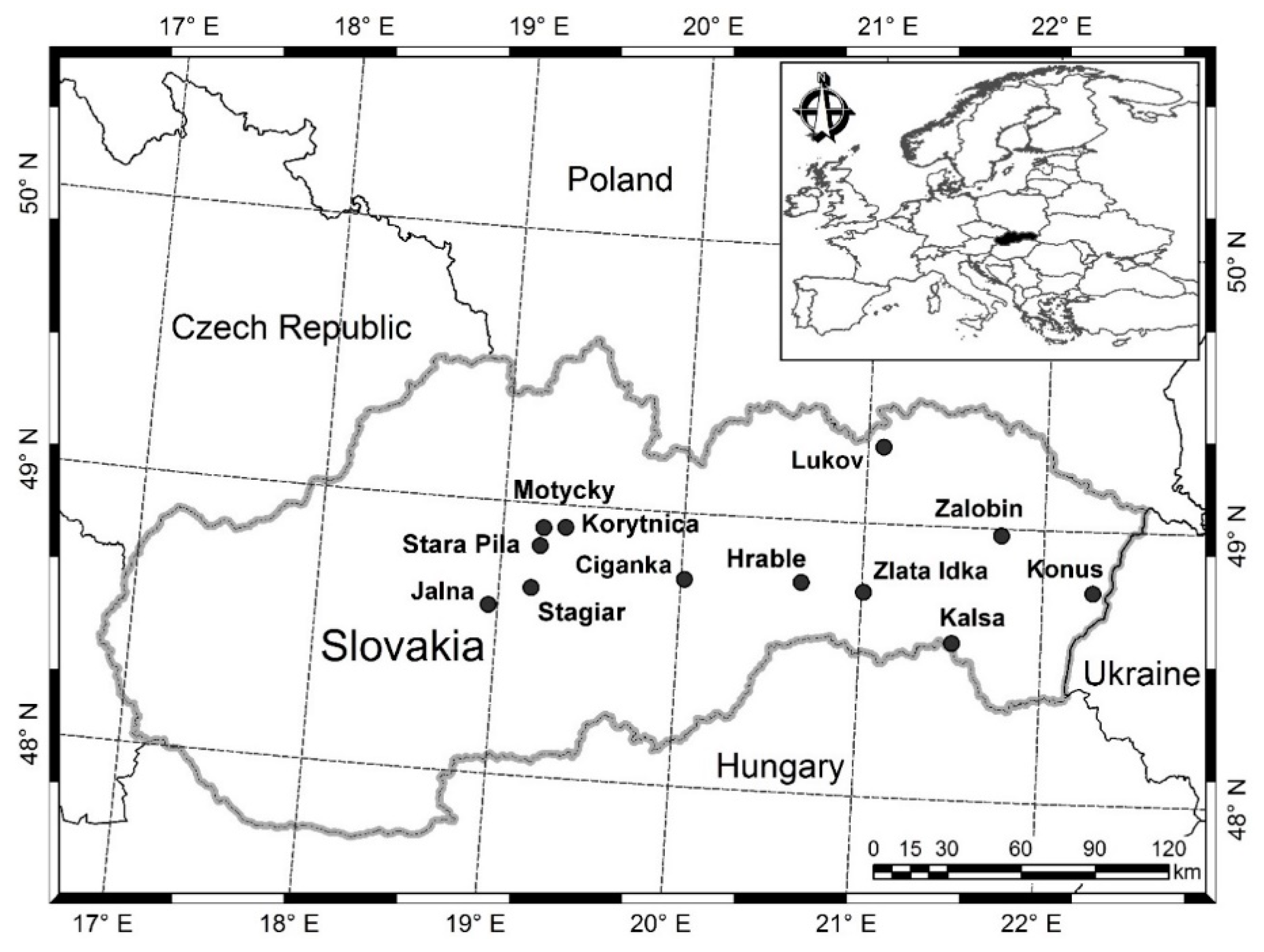
2.1. Data Materials

This study is based on the data originating from twelve thinning experiment sites (Figure 1), also named as long-term research plots (four long-term research plots comprising 15 sub-plots in the mixed (spruce-fir-beech) stands and eight long-term research plots comprising 26 sub-plots in the monospecific beech stands). Hereafter, sub-plots are termed as sample plots. The area of a squared-shaped sample plot was 0.25 ha (50 × 50 m). Sample plots are located on the sub-mountain vegetation zones, with elevation ranging from 250 to 700 m in the monospecific stands and 690–970 m in the mixed stands. Sample plots were established during 1958–1984 (Table 1). The studied forests, where sample plots were established, were chosen to meet these criteria, such as (i) they were originated from natural regeneration, (ii) no thinning was applied to the forests prior to the sample plot establishment, (iii) beech was as a dominating species in the stands (canopy cover ≥ 90%) and beech proportion by basal area ranged from 18% to 61% in the mixed stands, and (iv) stands were not older than 30–60 years in the monospecific stands, and 15–74 years in the mixed stands. The main objective of establishing sample plots was to study the effects of various thinning methods (Table 1) on wood production and timber quality of beech. At the time of sample plots establishment, stand age was 30–60 years in the monospecific stands, and 15–74 years in the mixed stands, but at present, stand age varies from 68 to 110 years (monospecific stands) and 65 to 127 years (mixed stands). The monospecific beech stands are mainly characterised by vegetation groups Fagetum pauper, Fagetum typicum, Fageto-abietinum and Querceto-Fagetum, and mixed beech stands by Fageto-Abietum, Fageto-Aceretum, and Abieto-Fagetum groups [37].
Two types of thinning [36]: (1) “C”—heavy thinning from below (following the principles defined by German forest research institute released in 1902); (2) “H” or “H2”—free crown thinning (thinning from above) were applied in 5- and 10-year’s interval, respectively, following the methods suggested by Štefančík [37]. At least one sample plot in each experimental site received no management intervention (control plot). The main principle of thinning lies in supporting the target trees (high quality trees) by removing their potential competitors. Detailed description of the stand treatments in our studied forests is available in Bosela et al. [24] and Štefančík et al. [36].
All trees with diameter at breast height (DBH ≥ 2.0 cm) were measured on each sample plot. All trees were numbered and point of DBH measurement was marked to reduce the measurement errors. Trees reaching DBH measurement threshold during study period were included, numbered, marked, and measured. Two DBH measurements were made perpendicular to each other and their average value was used. A transect of 50 m length and 10 m width was established on each sample plot, and tree height, height to crown base, and crown width were measured for all trees lying within the transect in each inventory cycle. Measurements were carried out in every five years.

2.2. Data Analysis

2.2.1. Tree and Stand Variables

We evaluated various variables that describe the effects of site quality, stand development stage, stand density and competition on the variation of diameter increment. We selected only those predictor variables, which contributed mostly to the diameter increment models. Some of the important variables were not measured in the field, such as dominant tree height and site index. We derived this information from measured data and models. We identified dominant trees from height measurements of sample trees on each sample plot using the methods suggested by Sharma et al. [23,38]. This method involves the ranking of height sample trees by height in the first stage and ranking by DBH in the second stage. In the third stage, mean rank is determined from both height and DBH ranks. The first few highest mean ranks are then used to identify the biggest trees (in terms of height and DBH). We chose the number of the biggest trees following the definition of dominant height (i.e., mean height of 250 largest trees per hectare, HDOM). Dominant diameter (mean DBH of dominant trees, DDOM) per sample plot was calculated. We also developed the dominant height-age model and estimated the site index, SI (HDOM at reference age of 100 years) using this model. Our intention of estimating SI was to use this as one of the covariate predictors in the diameter increment models. The HDOM-age model was developed using the generalized algebraic difference approach (GADA). The Hossfeld function [39] was used as a base function to develop GADA-based HDOM-age model [38,40]. The GADA allows for more than one parameter of a base function to be site-specific, and therefore resulting HDOM-age model generates the polymorphic curves with multiple asymptotes [38,40]. The GADA is also most suitable for modelling growth of tree- and stand-level attributes using short time-series data. Even if no common base age is available in the series, GADA allows for fitting HDOM-age series. This is the reason that GADA-based models are commonly known as base-age invariant models. However, fitting of HDOM-age of the short-time series is not possible with traditional approach (base-age specific approach) without interpolation or extrapolation of the height at base age. Presenting the derivation details of the GADA-based HDOM modelling here is out of the scope of this article. Readers may find them in the literature e.g., [38,40]. Final form of the GADA-based model we used to fit data is given below:
H 1 = b 1 + X 0 1 + b 2 X 0 T 1 b 3 + ε , X 0 = H 0 b 1 1 b 2 H 0 T 0 b 3
where H1 and H0 are dominant heights at the breast height age T1 and T0, respectively; ε is an error, and b1, b2, b3 are parameters to be estimated.
We calculated other stand-level variables and included into the models to describe the variations of diameter increment, such as stem number (N, ha−1), basal area (BA, m2 ha−1), arithmetic mean DBH (AMD, cm) and quadratic mean diameter (QMD, cm) per sample plot. We also calculated two tree-centered competition measures, such as ratio of DBH to QMD (Dq) and basal area of the trees larger in diameters than a subject tree (BAL, m2 ha−1). We calculated the relative spacing index (RSI) defined by R S I = 10000 / N H D O M . This is assumed as the most effective density measures, as it includes both stand stocking and stand development stage through N and HDOM, respectively [41,42,43]. We also calculated basal area proportion of a species of interest (BAPRO) and evaluated its potential contributions to the variations of diameter increment. All the stand measures, except HDOM and DDOM, were calculated using measurements of all trees regardless of species. It was not possible to calculate the distance dependent competition measures due to lack of tree coordinates in our data. Data used in our modelling are shown in Figure 2, and summary statistics including mean, minimum, maximum, and standard deviation of the important variables are given in Table 2. There is a data gap between stand age of 25 and 35 years, as two thinning experiments (Stara Píla and Konus) established on very young stands were measured in 1961 and 1966, but not in 1971 and 1976.

2.2.2. Tree Diameter Growth: A Theoretical Context and Modelling Approach

We developed both age independent and age dependent diameter increment models. The former model was developed with the expression of diameter increment as a function of DBH as a main predictor and other variables (Table 2) as covariate predictors, while the latter model includes stand age as an additional covariate predictor. Of all variables measured in the sample plots, diameter is probably the most harmonized one, available for the largest number of trees, available as repeated measurements on the same tree, and directly measured without further interpretation [44]. Tree diameters are commonly correlated with other tree-and stand-level variables that are relatively more difficult to measure, e.g., stem volume or tree biomass. Additionally, tree diameter can reflect the monetary worth of trees and competitive position of a tree within a stand [45]. Diameter growth rate of individual trees can be expressed as a diameter increment or basal area increment per year. The basal area increment models are often preferred over the diameter increment models, but Vanclay [3] and Schelhaas et al. [44] argue that both model types are essentially the same, since one can be derived from the other.
Tree growth is intrinsically exponential process in early age, but this, in the latter age, is constrained by action of two opposing forces: external environmental resistance and internal self-regulatory mechanism [46,47]. To describe the growth processes properly, two terms representing growth expansion and growth reduction need to be included into the growth models. The growth model possessing these two properties can be derived from the integral form of any mathematical functions by applying the derivative rules [46,47,48]. Generally, diameter of a tree develops according to asymmetric sigmoidal function through time, with relatively slow in the early age, but rapidly increasing growth at establishment, almost constant growth during the matured-phase followed by a slow decline of the growth during the senescence [44,49]. Since creating new tree rings is essential for water transport, and diameter increment will theoretically never reach zero, even though rings can be very small at old age [44]. We considered eight nonlinear integral functions (Table 3) to derive their incremental (differential) forms. These functions are commonly used to model the growth of tree- and stand-level attributes. Modelling of sigmoidal relationships is usually achieved with so-called theoretical growth curves, such as various exponential functions including Chapman-Richards functions [50,51,52,53,54,55]. In addition to these, we also evaluated three fractional forms of the functions: Näslund function [56], Levakovic function [57], and Hossfeld function [39]. With application of the derivative rules (i.e., change of a response variable with respect to size of a main predictor variable, DBH), we obtained the differential forms of all eight functions (see example, below in Equations (2)–(4)) and evaluated their fitting ability to our data.
Here, we prefer presenting both the differential and integral forms of the Chapman-Richards function as an example, which showed the best fitting performance to our data.
y = b 1 { 1 e x p ( b 2 x ) } b 3
Equation (2) is an integral form, if this function is differentiated with respect to x, following equation is evolved:
y = b 1   b 2   b 3   { 1 e x p ( b 2 x ) } b 3 1   e x p ( b 2 x )
In Equations (2) and (3), y = accumulative diameter growth (yield), x = DBH, y = diameter growth rate (increment per year), b1, b2, b3 are parameters to be estimated. Since Equation (3) does not describe the total variations of diameter increment, an error term, ɛ is necessary to represent the unexplained variation (Equation (4)). For simplicity, we applied ϕ = b 1   b 2   b 3 to Equation (4) and other functions in Table 3 in the same way or differently.
y = ϕ { 1 e x p ( b 2 x ) } b 3 1   e x p ( b 2 x ) + ε
Using DBH as a single predictor (x = DBH) and the dummy variable (SMR), which was included with ϕ expressed as a function of SMR, we fitted all the eight derivative forms of the functions (Table 3). There were many types of thinning applied to the stands (Table 1), however, the effect of each type could not be included through dummy variable modelling, as this increased the complexity and hindered the model convergence. Also, developing separate diameter increment model for each thinning type was not possible due to the limited observations. Thus, it was necessary to reduce the number of thinning types into two (control and thinning) in order to include them into the models using a dummy variable, SMR (SMR = 1 for thinned sample plots; otherwise 0). The Chapman-Richards function resulted in the least residual variations (i.e., smallest sum of squared errors), and therefore we selected this for further extension, aiming to increase the prediction accuracy of the diameter increment models.

2.2.3. Extension of Chapman-Richards Function

We investigated the potential contributions of various tree- and stand-level variables on the variations of diameter increment through their inclusion into the basic diameter increment models (Equation (4)). Our evaluation was based on whether the variables were suited to the model fitting procedure, which begins from the analysis of graphs and correlation statistics [21,58]. Among many potential covariate predictors (Table 2) evaluated, we found HDOM, BAPRO, stand age (A), SI, and Dq as the most significantly contributing ones based on the Akaike information criterion (AIC) and likelihood ratio test (LRT) [16,18,19,20]. The selected variables resulted in the smallest AIC, the largest log-likelihood and LRT in the model fitting. The problem of over-fitting (over-parameterization) was controlled by LRT and between-variable dependency was checked with correlation statistics. The expanded models provided the greatest fitting improvement when ϕ of a basic function (Equation (4)) was expressed as below (Equation (5)).
ϕ = f ( H D O M ,   A ,   B A P R O , S I ,   D q ,   S M R )
where HDOM = dominant height (m); BAPRO = basal area proportion of a species of interest (m2 ha−1); A = stand age (year); SI = site index defined by HDOM at the reference age of 100 years (m); Dq = ratio of DBH to quadratic mean diameter; SMR = stand management regime.
Our database contained the multiple sampling units (repeated measurements on the same tree, multiple trees in the same plot, and multiple plots in the same experiment), which would result in significant dependency among the observations of the same subject. We, therefore, formulated the mixed-effects models through the inclusion of random components that could account for variability and dependency among the observations within and across the sampling units. The main objective of inclusion of the random components into the models is to secure the higher prediction accuracy [16,59]. We formulated various mixed-effects model alternatives with all possible combination of the random effects and three fixed parameters in Equation (4) and fitted to data. The convergence with the smallest Akaike information criterion (AIC) and largest LRT was only possible when random effect parameters were added to ϕ and b3 of this equation. The procedure of formulating mixed-effects model is available in the standard textbooks [16,60]. We, therefore, present only the final forms of our mixed-effects models (Equations (6) and (7)) that described the largest variations of diameter increment in our data. The age independent and age dependent mixed-effects models are expressed by Equations (6) and (7), respectively.
y i j = ( ϕ + u i 1 ) { 1 e x p ( b 2 x i j ) } ( b 3 + u i 2 ) 1   e x p ( b 2 x i j ) + ϵ i j ,       ϕ = α 1 H D O M i α 2 + α 3 B A P R O i + α 4 S I i + α 5 D q i j + α 6 S M R i
y i j = ( ϕ + u i 1 ) { 1 e x p ( b 2 x i j ) } ( b 3 + u i 2 ) 1   e x p ( b 2 x i j ) + ϵ i j ,     ϕ = α 1 H D O M i α 2 + α 3 B A P R O i + α 4 S I i + α 5 D q i j + α 6 S M R i + α 7 A i
where y i j is a response variable (diameter increment, cm year−1); x i j is a main predictor variable (DBHij, cm); ϕ, bk (k = 2,3) and αk (k = 1,2,3,4) are parameters to be estimated; SMR is a dummy variable that accounts for the effect of the specific stand management regime (SMR = 1 for thinned sample plot; otherwise 0); ε i j is an error term; index i stands for ith sample plot; and j stands for jth tree; s stands for European beech, and all other abbreviations are the same as in Equation (5). The vectors of errors (εij) and random effects (ui1, ui2) are defined by ε i ~ N ( 0 ,   R i ) and u i ~ N ( 0 ,   D i ) , respectively. The vector εi is assumed to have normal distribution with zero mean and within-plot variance-covariance matrix R i and it is given by
R i = σ 2 G i 0.5 Г i G i 0.5
where σ2 is a scaling factor of error dispersion and equivalent to the residual variance of the estimated fixed-effect model and common to all sample plots [16,18]. A matrix Гi accounts for autoregressive error structure, which, in our case, was described by the first-order autoregressive error-structures, (AR(1)) defined by
AR ( 1 ) = σ 2 [ 1 ρ ρ 2 ρ 1 ρ ρ 2 ρ 1 ]
where ρ is the autoregressive parameter and σ2 is the same as defined in Equation (8).
A matrix Gi in Equation (8) accounts for heteroscedasticity; however, we did not observe the significant heteroscedasticity in our data when mixed-effects modelling was applied to estimate the parameters. The vector ui was assumed to have a multivariate normal distribution with zero mean and sample plot variance-covariance matrix D i and it is given by
D i = [ σ u i 1 2 σ u i 1 u i 2 σ u i 2 u i 1 σ u i 2 2 ]

2.2.4. Model Estimation and Evaluation

The base functions (Table 3) and dominant height-age model (Equation (1)) were estimated using the least square nonlinear regression in PROC NLIN of the SAS [61]. The mixed-effects model variants (Equations (6) and (7)) were estimated using the SAS macro NLINMIX [61] with expansion-around-zero method [62]. The restricted maximum likelihood was used, which is based on the linearization method through expanding the likelihood function of the nonlinear mixed-effects model with the first-order Taylor series approximation. We evaluated the fitting performance of the models using the root mean square error (RMSE), coefficient of determination (R2), and Akaike information criterion (AIC), which are common statistical measures for evaluating goodness-of-fit statistics. The RMSE analyzes the precision of estimation whereas R2 reflects the total variability described by model. Following the suggestion of Nakagawa and Schielzeth [63], we computed two types of coefficient of determinations: marginal coefficient of determination ( R m 2 ) and conditional coefficient of determination ( R c 2 ). The former describes the fixed-effects variance and later provides the variance described by both fixed- and random-effects in the mixed- effects models. The AIC is based on minimizing the Kullback-Lieber distance that imposes the penalty for a number of parameters included into the model [64]. We also analysed the residual graphs and simulated curves showing the effects of covariate predictors on the variations of diameter increment. Unless otherwise stated, we used 5% level of significance in our analyses. We also examined the calibrated (localized) diameter increment curves overlaid on the measured data for each sample plot.

2.2.5. Calibrated Response or Localized Diameter Increment Prediction
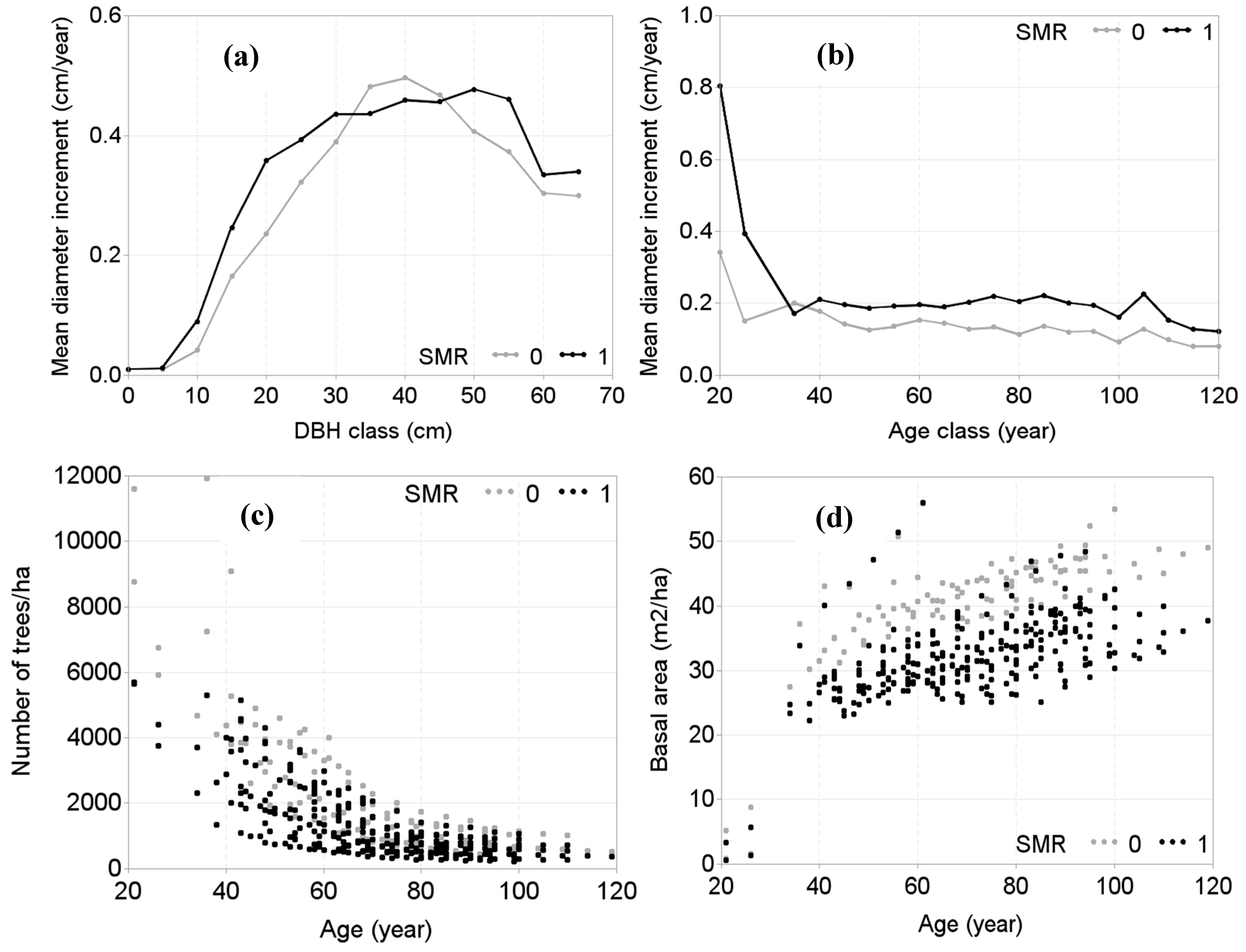
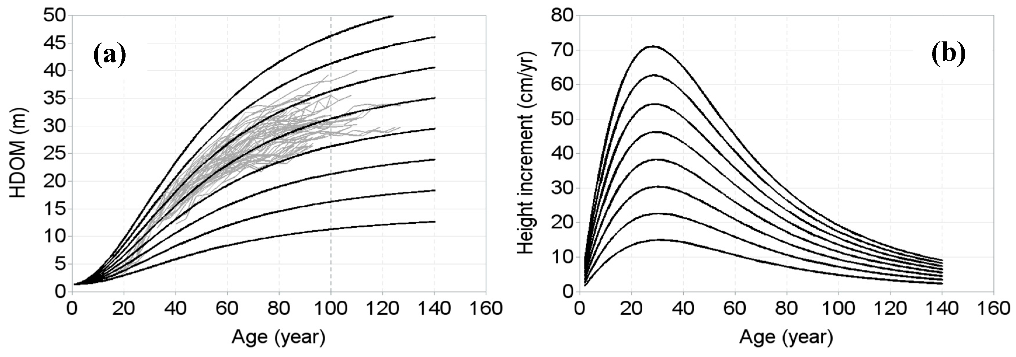
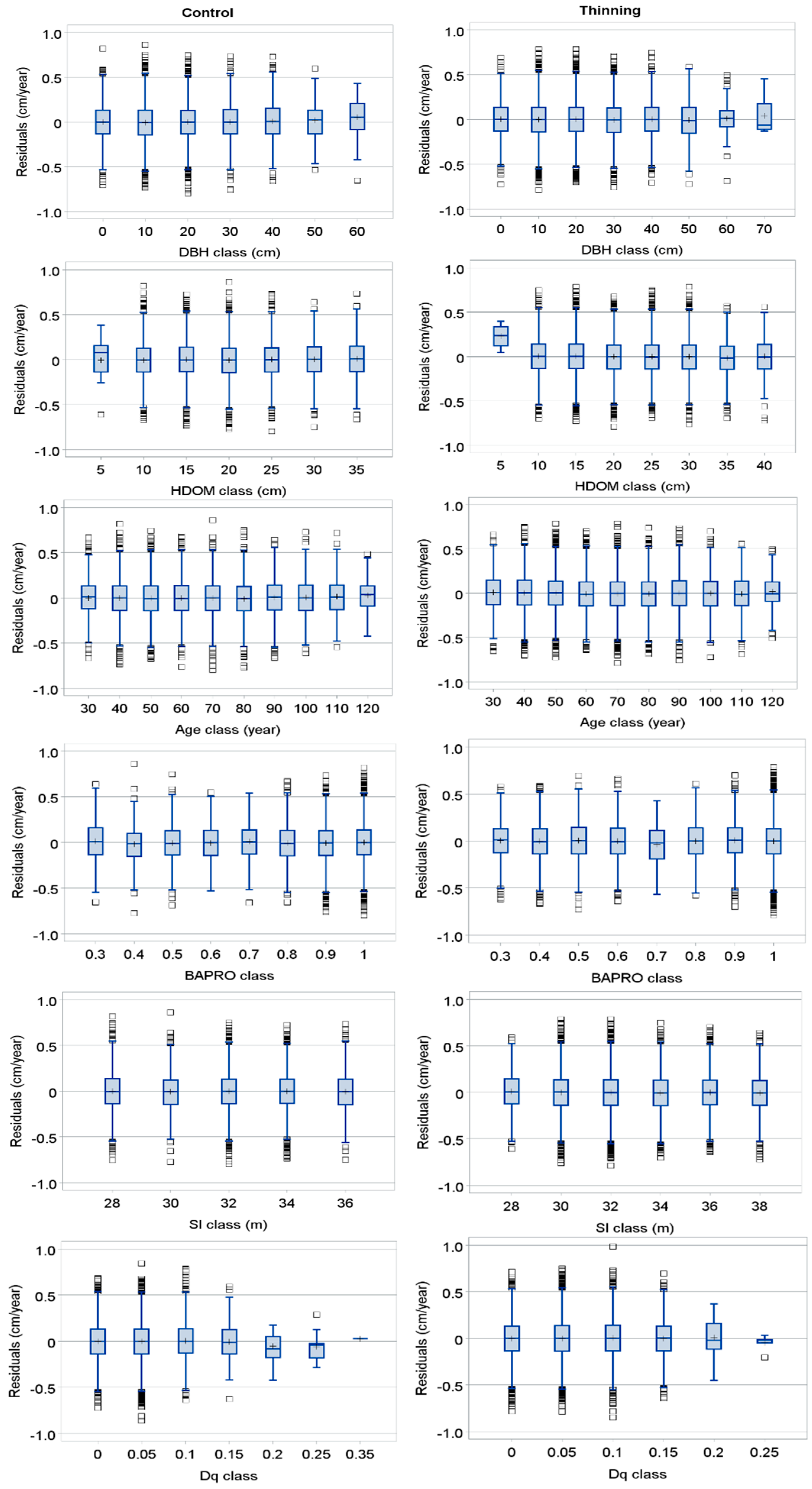
Predicting diameter increment with the random effects estimated from a prior measurement of a response variable ( y in Equations (6) and (7)) is known as calibration of the mixed-effects model [16,19]. The information of diameter growth per year from any number of beech trees per sample plot may be used for calibrating mixed-effects model. Although the higher the number of trees implies higher prediction accuracy, using a high number of sample trees in the calibration leads to higher inventory cost with a little improvement of predictive accuracy. Many studies of the mixed-effects modelling in forestry [18,20,21,22,23,38,42,59] have shown that prior measurements of four or five trees per sample plot would compromise between sampling cost and prediction accuracy. We also calibrated our mixed-effects diameter increment models using four randomly selected trees per sample plot. The empirical best linear unbiased prediction (EBLUP) equation (Equation (11)) was used to estimate the random effects in the model fitting data using the PROC IML in SAS [61].
u i = D Z i T ( Z i D Z i T + R i ) 1 ε i
where ui is a vector of the random effects, Equations (8) and (10) provide the elements of matrices R i   and   D , respectively. A vector ε i was obtained from fixed parts of the mixed-effects models (Equations (6) and (7)). A designed matrix, Zi is defined by
Z i = f ( x i ,   b , u i ) b
where b is a vector of the fixed parameters of equations (Equations (6) and (7)), uj is a vector of the random effects (ui1, ui2), and xi is a vector of the predictors for ith sample plot. The elements (zij) of this matrix for sample trees were determined from the partial derivatives of the nonlinear models (Equations (6) and (7)) with respect to the fixed parameters associated with the random effects [16,65,66,67]. Following equations were obtained from the partial derivative solution.
z i j ( ϕ ) = e x p ( b 2 x i j ) { 1 e x p ( b 2 x i j ) } b 3 1 z i j   ( b 3 ) = ϕ e x p ( b 2 x i j )   L n   { 1 e x p ( b 2 x i j ) } { 1 e x p ( b 2 x i j ) } b 3 1 , ϕ = α 1 H D O M i α 2 + + α 3 B A P R O i + α 4 S I i + α 5 D q i j + α 6 S M R i       and ϕ = α 1 H D O M i α 2 + α 3 B A P R O i + α 4 S I i + α 5 D q i j + α 6 S M R i + α 7 A i
All abbreviations and symbols are the same as in the previous equations.

3. Results

We estimated SI for each sample plot using the GADA-based HDOM-age model (Equation (1)). The parameterized HDOM-age model also known as SI model for European beech in the Slovakia would be
H 1 = 286.5117 + X 0 1 7.5583 X 0 T 1 1.889 + ε , X 0 = H 0 286.5117 1 + 7.55825 H 0 T 0 1.889
where H0 at the age T0 would be the SI for a sample plot with the measured H1. The SI curves and HDOM increment curves generated with Equation (14) are presented in Figure 3. This model described most parts of the variations in the HDOM-age relationships (R2adj = 0.9403; RMSE = 1.4513) without significant residual trends, and all parameter estimates were significant (p < 0.0001). The parameter accounting for the first-order autoregressive error-structure in the HDOM-age data was also significant (p < 0.0001).
In the first stage of modelling diameter increment, eight functions (Table 3) were considered as base functions and fitted to data using DBH as a main predictor and one dummy variable that accounts for the effect of the specific stand management regime as a covariate predictor. The Chapman-Richards function described the largest part of the variations of diameter increment with the smallest residual variation followed by Gompertz function (Table 4). However, difference in the fitting performance of other functions relative to the best was very small. The best fitted function, which was extended through introduction of the selected additional variables substantially increased the fitting improvement of the model. The fitting improvement of the extended Chapman-Richard model relative to its basic form increased by 59%, indicating that covariate predictors had the major contribution to the variations of diameter increment. Furthermore, when sample plot-level variations and randomness in the data were included into the extended models (Equations (6) and (7)) through application of the mixed-effects modelling, the fitting improvement in terms of the explained variance relative to that of the ordinary least square regression models increased by 16%. This indicated that sample plot-level variations and other stochastic factors had significant effects on the variations of diameter increment. The parameter estimates and fit statistics of the age independent and age dependent mixed-effects diameter increment models (Equations (6) and (7)) are presented in Table 5. The parameter estimates of all predictors are significantly different from zero (p < 0.05). The estimated value and sign of each parameter of both types of the models are biologically plausible and interpretable. The age dependent model described a slightly larger part of the variations of diameter increment than age independent model.
Box plots of the residuals plotted against each of the potential predictor variables (Table 2) were examined, however, for the brevity of space; only residuals plotted against the most contributing variables (DBH, HDOM, Age, BPRO, SI, and Dq) are presented here (Figure 4). Except for few cases (e.g., HDOM smaller than 10 m on the thinned sample plots and Dq larger than 0.15 on the control sample plots), no significant trend was observed in the residuals across the observed range of the predictor variables. None of the heteroscedasticity problems was observed either. The histograms of the residuals also showed the Gaussian distribution patterns (bell-shaped patterns), indicating that significant skewness was absent in the residuals.
Each covariate predictor significantly contributed to the variations of diameter increment (Figure 5). The maximum increment might occur at some point between DBH of 30 cm and 60 cm. Diameter increment significantly decreased with the advancement of the stand development stage (increased HDOM and stand age, AGE), decreasing species proportion of a species of interest (increased BAPRO). However, diameter increment increased with increasing site quality (increased SI) and decreasing competition and stand density (increased Dq). The magnitude of spacing between the consecutive increment curves on each panel of this figure suggests that there would be different influences of the covariate predictors (HDOM, A, BAPRO, SI, Dq) on the variations of diameter increment. The HDOM and AGE had the largest contributions, and BAPRO and SI had the smallest contributions to the diameter increment models.
We examined the sample plot-specific diameter increment curves produced with the calibrated mixed-effects model (localized age independent model) that were overlaid on the measured data (Figure 6). The increment curves would pass through the clouds of measured data, indicating that the calibrated model would be precise for the prediction of the diameter increment using the random effects estimated from prior measurements of four randomly selected trees per sample plot. However, this figure also shows that diameter increments for few very smaller trees having the fastest growth rate compared to others in the same sample plot are not properly described by model.
We also examined the prediction errors of the calibrated mixed-effects model for each stand management regime (Figure 7). This figure shows the absence of systematic bias for any individual regime, indicating that our mixed-effects models would be precise for each thinning type (Table 1).

4. Discussion

Tree growth is significantly influenced by various factors, such as physical, physiological and ecological factors [44]. We developed the mixed-effects nonlinear models describing diameter increment as a function of various variables describing individual tree-and stand-level characteristics and sample plot-level random effects. Based on the evaluation of the eight versatile growth functions (Table 3), which we considered as base functions based on the principles of their logical behavior and suitability in the practical application. The Chapman-Richards function, which shows the best fitting performance to our data (Table 4), has enough flexibility for modelling different tree attributes, such as growth of diameter and height [68,69,70,71] and height-diameter relationship [67,72,73].
A main predictor variable (DBH) describing more than one-third of the total variations of diameter increment (Table 4) indicates that DBH is tightly linked to the diameter increment. Other studies also find similar results when DBH was considered as a main predictor in the radial growth models developed for beech [44,74,75]. However, all these studies are based on the traditional (ordinary least square) regression fitting method, which is not appropriate for the hierarchically-structured data, as such fitting produces a significantly biased model [16]. The novelty of our models, therefore, lies beyond the traditional growth models of European beech [44,74], as our models are based on the mixed-effect modelling, which is the most appropriate for the hierarchically-structured data. The large values of the estimated variance and covariance components (Table 5) suggest that the mixed-effects modelling through the inclusion of the sample plot-level random effects and other stochastic variability is largely justifiable. For example, R c 2 of the mixed-effects model relative to its basic form fitted using DBH as a main predictor and one dummy variable increased from 0.40 to 0.66 (age independent) and to 0.68 for age dependent model. This suggests that the contribution of the covariate variables (HDOM, A, BAPRO, SI, Dq) and random effects to the variations of diameter increment is substantial and their effects cannot not be disregarded. The improvement in the model performance by introducing multiple predictors and random effects has been also reported by many others [13,76].
A description of a large part of the variations of diameter increment without significant residual trends (Table 5; Figure 4) indicates that the chosen base function (Chapman-Richards function) and covariate predictors, and modelling approach applied are all suited to our data. Even though fit statistics of the models could be marginally improved through introduction of additional covariate predictors, we did not over-parameterize our model, considering the fact this would lead to the biased estimation [77]. Only independent predictors, which are less correlated to each other must be selected to reduce the bias caused by over-parameterization. A parsimonious model with a high prediction precision is always the preferred choice for efficient application [3,71]. The parsimonious model could make the effort easier for the prediction of diameter increment from measurements of DBH and covariate predictors that can be derived from the routine forest inventories.
Different covariate predictors introduced in the models (Equations (6) and (7)) influence diameter growth differently (Figure 5). With advancing stand development stage through time on the given stand density and site quality, diameter increment of the trees would decrease, which is biologically plausible, as stands getting older would have a relatively slower diameter growth compared to height growth. Diameter increment is significantly influenced by stand density or competitive interaction among the trees, as they always compete for the limited resources, such as space, moisture, nutrients, and light. A large part of the explained variance in the diameter increment model is attributed to the variables related to the site quality (SI), stand density or competition (Dq), species mixture (BAPRO), and stand development stage (HDOM and A), which appear more influential to the diameter increment than many others, which we also evaluated (Table 2). This is in line with many other studies that have found the variables describing stand density and competition to be the important variables in describing diameter increment [44,75]. Diameter increment increases with decreasing competition as depicted by increased Dq (Figure 5), because of the crowding of trees within a stand that may result in taller heights and smaller crowns, but thinner boles. In attempt to get the higher canopy position for light, the subordinate trees have less diameter growth for the given unit of height growth as compared to the trees already grown to the top canopy position [78,79]. However, trees with dominant or codominant canopy positions may allocate more resources to diameter growth relative to height growth, and therefore have larger diameter increment and are more stable compared to the subordinate trees [80].
The effects of thinning would be substantial on the tree diameter growth [78,81] and other tree and stand characteristics [24,36]. Compared to the diameter increment on the control sample plots, that of the thinned sample plots was significantly larger and difference is clearly visible in our data and models (Figure 2, Figure 4, Figure 5 and Figure 6). It is due to the increased availability of the resources (light, moisture, nutrients, space) to the residual trees. The multiple dummy variables that could describe each of the all individual thinning types (Table 1) could not be included into our models, as this increased the models’ complexity and resulted in the non-convergence. Also, developing separate model for each thinning type was not possible due to inadequate number of observations. It was, thus, necessary to reduce the number of management regimes into two in order to make the models converged with significant parameter estimates. Even though our models include the effects of management regimes in a broader scale (control or thinning), these models can be applicable for the precise prediction of diameter increments for the stands managed with any thinning type and intensity. This is confirmed from analysis of the predication errors of our mixed-effects model that was calibrated with the random effects estimated using the measured diameter increment of four randomly selected trees per sample plot and applied to each management regime (Figure 7).
The effect of species mixture on the diameter increment is significant (p < 0.05). Diameter increment of the trees in the mixed stands increases with decreasing proportion of a species of interest (European beech), i.e., larger the number of tree species associated with beech in a stand could result in its faster diameter growth under the given stand density, site quality, and stand development stage (Figure 4). Most of our studied stands consist of multiple tree species ranging from 2 to 12 species. Therefore, it was necessary for us to include the species mixing effects into the diameter increment models. There could be the higher diameter increment of trees in the mixed stands, because inter-specific competition would not be more intense compared to the intra-specific competition in the monospecific stands. More intense competition may be experienced by trees in the less complex stands (monospecific stands or stands containing only a few tree species) compared to more complex stands (stands containing many tree species). The monospecific stands could have relatively less complex canopy structure, lower environmental variability within the stands, lower resource use efficiency and less resource capture capacity of the trees [82,83,84]. The mixed species stands are characterized with higher crown plasticity and complex canopy structure, which could trigger the plasticity at organ, crown or tree structure levels for the optimal capture of resources or acclimation to environmental conditions altered by competing neighbors [84]. The species mixture creates the neighborhood situation and structural heterogeneity where trees would acquire wider crown width, faster growth rate due to increased availability of resources [83,84]. Several studies investigated the species mixing effects on the variations of tree characteristics of European beech and other species and concluded that trees in the mixed species stands could have higher resource use efficiency, and therefore have remarkably higher growth rate compared to the trees in the monospecific stands [23,33,42,85,86,87,88].
As shown in Figure 6, our model provides a realistic prediction over a wide range of data, however, a precaution is necessary while applying the model beyond data range as data used for modelling do not fully cover the physiological rotation of beech stands. Size coverage of our data is limited up to 70 cm DBH (Figure 2), as beech may have grown to more than this size. This may result in less prediction precision of our models beyond this size. Even though radial growth models have been developed using a large dataset that covers the full range of growing conditions for several tree species including beech across Europe [44], beech stands in the Slovakia and other central European countries are not covered. In this situation, our models might be useful for effective management of beech forests, not only in the Slovakia, but also other countries where similar growing condition to the basis of this study would exist. When independent beech growth data are obtained from elsewhere in the central Europe, the prediction performance of our models may be compared against those of the recently developed diameter increment models [44].
The long-term research plots provide more accurate growth data than those supplied by other types of sampling designs, such as the national forest inventory (NFI) sample plots. However, for many years, access to data originating from long-term research plots has been limited, as establishing these sample plots and operating them is expensive. In this context, our models, which are based on the long-term research plots, will provide good opportunity to the researchers for comparing their models developed using data originating from other databases (e.g., NFI and stem analysis). We used some simplifying assumptions to develop our models, such as linear diameter growth between two consecutive measurements, which may reduce the prediction precision. Since it is imperative to include climatic variables to make the growth model climate sensitive, we were not able to do this due to lack of climate data. It is well known that validation provides the credibility of the developed models, however, we were not allowed to do this due to the lack of external independent data. Even though validation may be carried out by splitting dataset, we did not do this either, assuming that splitting data does not provide more information in addition to the respective fit statistics obtained directly from estimation of the models using entire dataset [89,90]. It is because that divided parts of the same dataset cannot be independent to each other, as they have similar statistical characteristics. Thus, validation of the models using the data acquired from different sampling design and tree population may be the best alternative [3,21,38,67]. Developing highly precise individual tree growth models may be challenging, because of several influential factors, which are not readily measured [10]. Any limitation experienced in the current study will be useful for improvement of the future modelling works.
Forests are dynamic ecosystems and prediction of those dynamics cannot be achieved through the individual tree diameter increment models only. Other individual tree-based models, such as recruitment and mortality models are also necessary to describe forest dynamics in details. Together with other forest models, our diameter increment models and site index model will be used for growth simulator to be developed in the future, which is a fundamental tool for decision-making in forestry. Being the spatially inexplicit type, our diameter increment models allow for easy computation during application and evaluation of the effects of various management alternatives.

5. Conclusions

We developed both age independent and age dependent diameter increment models for European beech using long-term research sample plot data in the Slovak Republic. We used diameter at breast height as a main predictor and stand-level variables: site index, stand age, dominant height, basal area proportion of a species of interest (European beech), and ratio of diameter at breast height to quadratic mean diameter as covariate predictors. A dummy variable was included into the models to describe the stand management regime-specific variations on the diameter increment. The sample plot-level random effects and the first-order autoregressive error-structure were also included using the mixed-effects modelling. The results showed that diameter increment was influenced significantly differently by different covariate predictors. Diameter increment decreased with advancement of the stand development stage, increasing stand density and competition, but increased with decreasing proportion of European beech in a stand and increasing site quality. Our diameter increment models are simple and will be applied for the precise prediction of diameter increments of the beech stands managed with any type of thinning using the measurements of diameter at breast height and other covariate predictors, which can be derived from the routine forest inventory databases.
The presented site index model can be used for evaluation of the potential site productivity of beech forests and diameter increment models can be used for simulation of beech stand dynamics across the Slovakia. Together with other forest models, our diameter increment models and site index model may be used for growth simulator to be developed in the future. Our models will be useful for formulation and implementation of silvicultural strategies of European beech, as these models are based on long-term growth data (over 50 years) that were acquired from the complex stands managed with various types of thinning. The structurally complex stands may have higher ability to tolerate the negative effects of climate change. Many other implications of the individual tree diameter increment models are briefly mentioned in the introduction and discussion sections of this article.

Author Contributions

R.P.S. conceptualized and designed the study, performed data analysis and modelling, wrote the manuscript and revised it; I.S. provided data and administered the project; I.S., Z.V., and S.V. contributed to data description and manuscript improvement, produced study area map, and contributed to revision of the manuscript.

Funding

This study was supported by the Slovak Research and Development Agency under contract (No. APVV-15-0032) and Faculty of Forestry and Wood Sciences, Czech University of Life Sciences in Prague (EVA4.0 project No. CZ.02.1.01/0.0/0.0/16_019/0000803, IGA No. B_19_05 and Excellent Output 2019).

Acknowledgments

We thank three anonymous reviewers for their constructive comments and insightful suggestions to improve our article.

Conflicts of Interest

The authors declare no conflict of interest.

References

  1. Garcia, O. The state-space approach in growth modeling. Can. J. For. Res. 1994, 24, 1894–1903. [Google Scholar] [CrossRef]
  2. Amaro, A.; Reed, D.; Soares, P. Modelling forest systems; CABI Publishing: Wallingford, Oxon, UK, 2003; p. 432. [Google Scholar]
  3. Vanclay, J.K. Modelling forest growth and yield: Applications to mixed tropical forests; CAB International: Wallingford, Oxon, UK, 1994; p. 312. [Google Scholar]
  4. Pretzsch, H. Forest dynamics, growth and yield: from measurement to model; Springer Verlag: Berlin/Heidelberg, Germany, 2009; p. 664. [Google Scholar]
  5. Weiskittel, A.R.; Hann, D.W.; Kershaw, J.A.; Vanclay, J.K. Forest growth and yield modeling; Wiley: New York, NY, USA, 2011; p. 424. [Google Scholar]
  6. Hasenauer, H.E. Sustainable forest management: growth models for Europe; Springer-Verlag: Berlin/Heidelberg, Germany, 2006; p. 388. [Google Scholar]
  7. Adame, P.; Hynynen, J.; Cañellas, I.; del Río, M. Individual-tree diameter growth model for rebollo oak (Quercus pyrenaica Willd.) coppices. For. Ecol. Manag. 2008, 255, 1011–1022. [Google Scholar] [CrossRef]
  8. Crecente-Campo, F.; Soares, P.; Tomé, M.; Dieguez-Aranda, U. Modelling annual individual-tree growth and mortality of Scots pine with data obtained at irregular measurement intervals and containing missing observations. For. Ecol. Manag. 2010, 260, 1965–1974. [Google Scholar] [CrossRef] [Green Version]
  9. Subedi, N.; Sharma, M. Individual-tree diameter growth models for black spruce and jack pine plantations in northern Ontario. For. Ecol. Manag. 2011, 261, 2140–2148. [Google Scholar] [CrossRef]
  10. Vospernik, S. Possibilities and limitations of individual-tree growth models—A review on model evaluations. Die Bodenkultur: J. Land Manag., Food Environ. 2017, 68, 103–112. [Google Scholar] [CrossRef]
  11. Sánchez-González, M.; del Río, M.; Canellas, I.; Montero, G. Distance independent tree diameter growth model for cork oak stands. For. Ecol. Manag. 2006, 225, 262–270. [Google Scholar] [CrossRef]
  12. Hasenauer, H. Concepts within tree growth modeling. In Sustainable forest management: Growth models for Europe; Hasenauer, H., Ed.; Springer Verlag: Berlin/Heidelberg, Germany, 2006; p. 398. [Google Scholar]
  13. Condés, S.; Sterba, H. Comparing an individual tree growth model for Pinus halepensis Mill. in the Spanish region of Murcia with yield tables gained from the same area. Eur. J. For. Res. 2008, 127, 253–261. [Google Scholar] [CrossRef]
  14. Sterba, H.; Monserud, R.A. Applicability of the forest stand growth simulator PROGNAUS for the Austrian part of the Bohemian Massif. Ecol. Model. 1997, 98, 23–34. [Google Scholar] [CrossRef]
  15. Hasenauer, H.; Kindermann, G.; Steinmetz, P. The tree growth model MOSES 3.0. In Sustaianble forest management, Growth models for Europe; Hasenauer, H., Ed.; Springer Verlag: Berlin/Heidelberg, Germany, 2006; p. 388. [Google Scholar]
  16. Pinheiro, J.C.; Bates, D.M. Mixed-effects models in S and S-PLUS; Springer: Berlin/Heidelberg, Germany, 2000. [Google Scholar]
  17. Saud, P.; Lynch, T.B.; Anup, K.C.; Guldin, J.M. Using quadratic mean diameter and relative spacing index to enhance height-diameter and crown ratio models fitted to longitudinal data. Forestry 2016, 89, 215–229. [Google Scholar] [CrossRef]
  18. Fu, L.; Sharma, R.P.; Hao, K.; Tang, S. A generalized interregional nonlinear mixed-effects crown width model for Prince Rupprecht larch in northern China. For. Ecol. Manag. 2017, 389, 364–373. [Google Scholar] [CrossRef]
  19. Hall, D.B.; Bailey, R.L. Modeling and prediction of forest growth variables based on multilevel nonlinear mixed models. For. Sci. 2001, 47, 311–321. [Google Scholar]
  20. Fu, L.; Sun, H.; Sharma, R.P.; Lei, Y.; Zhang, H.; Tang, S. Nonlinear mixed-effects crown width models for individual trees of Chinese fir (Cunninghamia lanceolata) in south-central China. For. Ecol. Manag. 2013, 302, 210–220. [Google Scholar] [CrossRef]
  21. Sharma, R.P.; Breidenbach, J. Modeling height-diameter relationships for Norway spruce, Scots pine, and downy birch using Norwegian national forest inventory data. For. Sci. Technol. 2015, 11, 44–53. [Google Scholar] [CrossRef]
  22. Sharma, R.P.; Vacek, Z.; Vacek, S.; Podrázský, V.; Jansa, V. Modelling individual tree height to crown base of Norway spruce (Picea abies (L.) Karst.) and European beech (Fagus sylvatica L.). PLoS ONE 2017, 12, e0186394. [Google Scholar] [CrossRef]
  23. Sharma, R.P.; Vacek, Z.; Vacek, S. Individual tree crown width models for Norway spruce and European beech in Czech Republic. For. Ecol. Manag. 2016, 366, 208–220. [Google Scholar] [CrossRef]
  24. Bosela, M.; Štefančík, I.; Petráš, R.; Vacek, S. The effects of climate warming on the growth of European beech forests depend critically on thinning strategy and site productivity. Agric. For. Meteorol. 2016, 222, 21–31. [Google Scholar] [CrossRef]
  25. Geßler, A.; Keitel, C.; Kreuzwieser, J.; Matyssek, R.; Seiler, W.; Rennenberg, H. Potential risks for European beech (Fagus sylvatica L.) in a changing climate. Trees 2007, 21, 1–11. [Google Scholar] [CrossRef]
  26. Knoke, T.; Ammer, C.; Stimm, B.; Mosandl, R. Admixing broadleaved to coniferous tree species: a review on yield, ecological stability and economics. Eur. J. For. Res. 2008, 127, 89–101. [Google Scholar] [CrossRef]
  27. Barna, M.; Ján, K.; Bublinec, E. Beech and Beech Ekosystems of Slovakia; VEDA: Bratislava, Slovak Republic, 2011; p. 634. [Google Scholar]
  28. Green report. Správa o lesnom hospodárstve v Slovenskej republike za rok 2016. Bratislava MPRV SR: 68. , 2017. Available online: https://www.enviroportal.sk/environmentalne-temy/vplyvy-na-zp/lesnictvo/dokumenty/spravy-o-lesnom-hospodarstve-v-slovenskej-republike (accessed on 23 May 2019).
  29. Vacek, Z.; Vacek, S.; Bílek, L.; Remeš, J.; Štefančík, I. Changes in horizontal structure of natural beech forests on an altitudinal gradient in the Sudetes. Dendrobiology 2015, 73, 33–45. [Google Scholar] [CrossRef] [Green Version]
  30. Petritan, A.M.; Von Lüpke, B.; Petritan, I.C. Effects of shade on growth and mortality of maple (Acer pseudoplatanus), ash (Fraxinus excelsior) and beech (Fagus sylvatica) saplings. Forestry 2007, 80, 397–412. [Google Scholar] [CrossRef]
  31. Bolte, A.; Hilbrig, L.; Grundmann, B.; Kampf, F.; Brunet, J.; Roloff, A. Climate change impacts on stand structure and competitive interactions in a southern Swedish spruce–beech forest. Eur. J. For. Res. 2010, 12, 261–276. [Google Scholar] [CrossRef]
  32. Bosela, M.; Tobin, B.; Šebeň, V.; Petráš, R.; Larocque, G.R. Different mixtures of Norway spruce, silver fir, and European beech modify competitive interactions in central European mature mixed forests. Can. J. For. Res. 2015, 45, 1577–1586. [Google Scholar] [CrossRef]
  33. Pretzsch, H.; del Rio, M.; Schütze, G.; Ammer, C.; Annighöfer, P.; Avdagic, A.; Barbeito, I.; Bielak, K.; Brazaitis, G.; Coll, L.; et al. Mixing of Scots pine (Pinus sylvestris L.) and European beech (Fagus sylvatica L.) enhances structural heterogeneity, and the effect increases with water availability. For. Ecol. Manag. 2016, 373, 149–166. [Google Scholar] [CrossRef]
  34. Hanewinkel, M.; Cullmann, D.A.; Schelhaas, M.J.; Nabuurs, G.J.; Zimmermann, N.E. Climate change may cause severe loss in the economic value of European forest land. Nat. Clim. Chang. 2013, 3, 203. [Google Scholar] [CrossRef]
  35. Boncina, A.; Kadunc, A.; Robic, D. Effects of selective thinning on growth and development of beech (Fagus sylvatica L.) forest stands in south-eastern Slovenia. Ann. For. Sci. 2007, 64, 47–57. [Google Scholar] [CrossRef]
  36. Štefančík, I.; Vacek, Z.; Sharma, R.P.; Vacek, S.; Rösslová, M. Effect of thinning regimes on development and growth of crop trees in Fagus sylvatica stands of Central Europe over 50 years. Dendrobiology 2018, 79, 141–155. [Google Scholar] [CrossRef]
  37. Štefančík, I. Rast, štruktúra a produkcia bukových porastov srozdielnym režimom výchovy (Vedecká monografia); NLC: Zvolen, 2015; p. 148. Available online: http://sclib.svkk.sk/sck01/Record/000499076 (accessed on 23 May 2019).
  38. Sharma, R.P.; Brunner, A.; Eid, T.; Øyen, B.-H. Modelling dominant height growth from national forest inventory individual tree data with short time series and large age errors. For. Ecol. Manag. 2011, 262, 2162–2175. [Google Scholar] [CrossRef]
  39. Hossfeld, J.W. Mathematik für Forstmänner, Őkonomen und Cameralisten; Nabu Press: Gotha, Germany, 1822; p. 310. [Google Scholar]
  40. Cieszewski, C.J. Comparing fixed- and variable-base-age site equations having single versus multiple asymptotes. For. Sci. 2002, 48, 7–23. [Google Scholar]
  41. Zhao, D.; Kane, M.; Borders, B.E. Crown ratio and relative spacing relationships for loblolly pine plantations. Open J. For. 2012, 2, 101–115. [Google Scholar] [CrossRef]
  42. Sharma, R.P.; Bíllek, L.; Vacek, Z.; Vacek, S. Modelling crown width-diameter relationship for Scots pine in the central Europe. Trees 2017, 31, 1875–1889. [Google Scholar] [CrossRef]
  43. Fonseca, T.F.; Duarte, J.C. A silvicultural stand density model to control understory in maritime pine stands. iForest 2017, 10, 829–836. [Google Scholar] [CrossRef] [Green Version]
  44. Schelhaas, M.-J.; Hengeveld, G.M.; Heidema, N.; Thürig, E.; Rohner, B.; Vacchiano, G.; Vayreda, J.; Redmond, J.; Socha, J.; Fridman, J.; et al. Species-specific, pan-European diameter increment models based on data of 2.3 million trees. For. Ecosyst. 2018, 5, 21. [Google Scholar] [CrossRef]
  45. West, P.W. Tree and forest measurement; Springer: Berlin/Heidelberg, Germany, 2009. [Google Scholar]
  46. Zeide, B. Analysis of growth equations. For. Sci. 1993, 39, 594–616. [Google Scholar] [CrossRef]
  47. Zeide, B. Accuracy of equations describing diameter growth. Can. J. For. Res. 1989, 19, 1283–1286. [Google Scholar] [CrossRef]
  48. Gyawali, A.; Sharma, R.P.; Bhandari, S.K. Individual tree basal area growth models for Chir pine (Pinus roxberghii Sarg.) in western Nepal. J. For. Sci. 2015, 61, 535–543. [Google Scholar] [CrossRef]
  49. Tomé, J.; Tomé, M.; Barreiro, S.; Paulo, J.A. Age-independent difference equations for modelling tree and stand growth. Can. J. For. Res. 2006, 36, 1621–1630. [Google Scholar] [CrossRef]
  50. Richards, F.J. A flexible growth function for empirical use. J. Exp. Bot. 1959, 10, 290–300. [Google Scholar] [CrossRef]
  51. Chapman, D.G. Statistical Problems in Dynamics of Exploited Fisheries Populations. Proceedings of the Fourth Berkeley Symposium on Mathematical Statistics and Probability; Neyman, J., Ed.; University of California Press: Berkeley, CA, USA, 1961; pp. 153–168. [Google Scholar]
  52. Bertalanffy, L. Quantitative laws in metabolism and growth. Quart. Rev. Biol. 1957, 32, 217–231. [Google Scholar] [CrossRef]
  53. Weibull, W. A statistical distribution function of wide applicability. J. Appl. Mech. 1951, 18, 293–296. [Google Scholar]
  54. Gompertz, B. On the nature of the function expressive of the law of human mortality and on a new model of determining life contingencies. Phil. Trans. R. Soc. 1825, 115, 513–585. [Google Scholar]
  55. Korf, V. A mathematical definition of stand volume growth law (In Czech). Lesnicka Prace 1939, 18, 337–339. [Google Scholar]
  56. Näslund, M. Skogsforsö ksastaltens gallringsforsök i tallskog (Thinning experiments in pine forest conducted by the forest experiment station). Medd. fran Statens Skogsforsöksanstalt 1936, 29, 1–169. [Google Scholar]
  57. Levakovic, A. An analytical form of growth law. Glasnik za Sumske Pokuse (In Serbo-Croat.) 1935, 4, 283–310. [Google Scholar]
  58. Fu, L.; Sharma, R.P.; Wang, G.; Tang, S. Modelling a system of nonlinear additive crown width models applying seemingly unrelated regression for Prince Rupprecht larch in northern China. For. Ecol. Manag. 2017, 386, 71–80. [Google Scholar] [CrossRef]
  59. Sharma, R.P.; Vacek, Z.; Vacek, S. Generalized nonlinear mixed-effects individual tree crown ratio models for Norway spruce and European beech. Forests 2018, 9, 555. [Google Scholar] [CrossRef]
  60. Vonesh, E.F.; Chinchilli, V.M. Linear and nonlinear models for the analysis of repeated measurements; Marcel Dekker: New York, NY, USA, 1997. [Google Scholar]
  61. SAS Institute Inc. SAS/ETS1 9.1.3 User’s Guide; SAS Institute Inc.: Cary, NC, USA, 2012. [Google Scholar]
  62. Littell, R.C.; Milliken, G.A.; Stroup, W.W.; Wolfinger, R.D.; Schabenberger, O. SAS for mixed models, 2nd ed.; SAS Institute: Cary, NC, USA, 2006; p. 814. [Google Scholar]
  63. Nakagawa, S.; Schielzeth, H. A general and simple method for obtaining R2 from generalized linear mixed-effects models. Methods Ecol. Evol. 2013, 4, 133–142. [Google Scholar] [CrossRef]
  64. Akaike, H. A new look at statistical model identification. IEEE Trans. Autom. Control 1974, 19, 716–723. [Google Scholar] [CrossRef]
  65. Calama, R.; Montero, G. Interregional nonlinear height-diameter model with random coefficients for stone pine in Spain. Can. J. For. Res. 2004, 34, 150–163. [Google Scholar] [CrossRef]
  66. Crecente-Campo, F.; Tomé, M.; Soares, P.; Dieguez-Aranda, U. A generalized nonlinear mixed-effects height-diameter model for Eucalyptus globulus L. in northwestern Spain. For. Ecol. Manag. 2010, 259, 943–952. [Google Scholar] [CrossRef]
  67. Sharma, R.P.; Vacek, Z.; Vacek, S.; Kučera, M. Modelling individual tree height-diameter relationships for multi-layered and multi-species forests in central Europe. Trees 2018, 33, 103–119. [Google Scholar] [CrossRef]
  68. Carmean, W.H.; Lenthall, D.J. Height growth and site index curves ofr jack pine in north central Ontario. Can. J. For. Res. 1989, 19, 215–224. [Google Scholar] [CrossRef]
  69. Goelz, J.C.G.; Burk, T.E. Development of a well-behaved site index equation-Jack pine in North central Ontario. Can. J. For. Res. 1992, 22, 776–784. [Google Scholar] [CrossRef]
  70. Huang, S.; Titus, S.J. An age-independent individual tree height prediction model for boreal spruce-aspen stands in Alberta. Can. J. For. Res. 1994, 24, 1295–1301. [Google Scholar] [CrossRef]
  71. Burkhart, H.E.; Tomé, M. Modeling forest trees and stands; Springer: Berlin/Heidelberg, Germany, 2012. [Google Scholar]
  72. Fang, Z.X.; Bailey, R.L. Height-diameter models for tropical forests on Hainan Island in southern China. For. Ecol. Manag. 1998, 110, 315–327. [Google Scholar] [CrossRef]
  73. Sharma, M.; Parton, J. Height-diameter equations for boreal tree species in Ontario using a mixed-effects modeling approach. For. Ecol. Manag. 2007, 249, 187–198. [Google Scholar] [CrossRef]
  74. Monserud, R.A.; Sterba, H. A basal area increment model for individual trees growing in even- and uneven-aged forest stands in Austria. For. Ecol. Manag. 1996, 80, 57–80. [Google Scholar] [CrossRef]
  75. Cienciala, E.; Russ, R.; Santruckova, H.; Altman, J.; Kopacek, J.; Hůnová, I.; Štěpánek, P.; Oulehle, F.; Tumajer, J.; Ståhl, G.R. Discerning environmental factors affecting current tree growth in Central Europe. Sci. Total Environ. 2016, 573, 541–554. [Google Scholar] [CrossRef]
  76. Zhao, L.; Li, C.; Tang, S. Individual-tree diameter growth model for fir plantations based on multi-level linear mixed effects models across southeast China. J. For. Res. 2013, 18, 305–315. [Google Scholar] [CrossRef]
  77. Dormann, C.F.; Elith, J.; Bacher, S.; Buchmann, C.; Carl, G.; Carre, G.; Marquez, J.R.G.; Gruber, B.; Lafourcade, B.; Leitao, P.J. Collinearity: A review of methods to deal with it and a simulation study evaluating their performance. Ecography 2013, 36, 27–46. [Google Scholar] [CrossRef]
  78. Mäkinen, H.; Nöjd, P.; Isomäki, A. Radial, height and volume increment variation in Picea abies (L.) Karst. Stands with varying thinning intensities. Scand. J. For. Res. 2002, 17, 304–316. [Google Scholar] [CrossRef]
  79. Sharma, R.P.; Vacek, Z.; Vacek, S. Modeling individual tree height to diameter ratio for Norway spruce and European beech in Czech Republic. Trees 2016, 30, 1969–1982. [Google Scholar] [CrossRef]
  80. Wonn, H.T.; O’Hara, K.L. Height: Diameter ratios and stability relationships for four northern rocky mountain tree species. West. J. Appl. For. 2001, 16, 87–94. [Google Scholar]
  81. Kim, M.; Lee, W.-K.; Kim, Y.-S.; Lim, C.-H.; Song, C.; Park, T.; Son, Y.; Son, Y.-M. Impact of thinning intensity on the diameter and height growth of Larix kaempferi stands in central Korea. For. Sci. Technol. 2016, 12, 77–87. [Google Scholar]
  82. Binkley, D.; Stape, J.L.; Ryan, M.G. Thinking about efficiency of resource use in forests. For. Ecol. Manag. 2004, 193, 5–16. [Google Scholar] [CrossRef]
  83. Bayer, D.; Seifert, S.; Pretzsch, H. Structural crown properties of Norway spruce (Picea abies [L.] Karst.) and European beech (Fagus sylvatica [L.]) in mixed versus pure stands revealed by terrestrial laser scanning. Trees 2013, 27, 1035–1047. [Google Scholar] [CrossRef]
  84. Pretzsch, H. Canopy space filling and tree crown morphology in mixed-species stands compared with monocultures. For. Ecol. Manag. 2014, 327, 251–264. [Google Scholar] [CrossRef] [Green Version]
  85. Pretzsch, H.; Block, J.; Dieler, J.; Dong, P.H.; Kohnle, U.; Nagel, J.; Spellmann, H.; Zingg, A. Comparison between the productivity of pure and mixed stands of Norway spruce and European beech along an ecological gradient. Ann. For. Sci. 2010, 67, 712. [Google Scholar] [CrossRef]
  86. Sterba, H.; del Rio, M.; Brunner, A.; Condes, S. Effect of species proportion definition on the evaluation of growth in pure vs. mixed stands. For. Syst. 2014, 23, 547–559. [Google Scholar] [CrossRef]
  87. Pretzsch, H.; Forrester, D.I.; Rötzer, T. Representation of species mixing in forest growth models. A review and perspective. Ecol. Model. 2015, 313, 276–292. [Google Scholar] [CrossRef] [Green Version]
  88. Sharma, R.P.; Vacek, Z.; Vacek, S. Modelling tree crown-to-bole diameter ratio for Norway spruce and European beech. Silva Fenn. 2017, 51, 1740. [Google Scholar] [CrossRef]
  89. Kozak, A.; Kozak, R. Does cross validation provide additional information in the evaluation of regression models? Can. J. For. Res. 2003, 33, 976–987. [Google Scholar] [CrossRef]
  90. Yang, Y.Q.; Monserud, R.A.; Huang, S.M. An evaluation of diagnostic tests and their roles in validating forest biometric models. Can. J. For. Res. 2004, 34, 619–629. [Google Scholar] [CrossRef]
Figure 1. Location of long-term research plots.
Forests 10 00451 g001
Figure 2. Mean diameter increments calculated by diameter at breast height (DBH) class with 5 cm interval (a) and age class with a five-year interval (b), number of trees per hectare per measurement cycle (c), and stand basal area per hectare per measurement cycle (d). DBH= diameter at breast height; SMR = stand management regime (SMR 0 = control sample plots; SMR 1= thinned sample plots).
Forests 10 00451 g002
Figure 3. Dominant height (HDOM) development curves overlaid on the measured HDOM data (a); HDOM increment curves for site index classes formed with 5 m interval between 12 m and 47 m (b).
Forests 10 00451 g003
Figure 4. Box plots of the standardized residuals of the mixed-effects model. Length of larger box represents the interquartile range (IQR), length of whisker represents class minimum and maximum values in the IQR, and smaller boxes represent the observations 1.5 times beyond the IQR (outlier observations lying far away from the median) and horizontal lines and plus signs in a larger box represent class median and mean values, respectively. DBH: Diameter at breast height; HDOM: dominant height; BAPRO: Basal area proportion of a species of interest; SI: Site index; Dq: Ratio of DBH to quadratic diameter.
Forests 10 00451 g004
Figure 5. Effects of dominant height (HDOM), stand age (AGE), basal area proportion of a species of interest (BAPRO), site index (SI), ratio of DBH to quadratic mean diameter (Dq) on the diameter increment, DBH: diameter at breast height. Curves were produced using the parameter estimates in Table 5 (only fixed parts of the mixed-effects model). Mean values of the data were used for predictors except variable of interest in the figure, which was allowed varying from approximately minimum to maximum in the measured data.
Forests 10 00451 g005
Figure 6. Sample plot-specific diameter increment curves overlaid on the measured diameter increment data. Sample plot mean of the covariate predictors, except the dominant height (HDOM), which was allowed varying from approximately minimum to maximum by 2 m in the measured data, were used to produce the curves. Model was calibrated with the random effects estimated using the measured diameter increment of four randomly selected trees per sample plot; DBH: diameter at breast height.
Forests 10 00451 g006
Figure 7. Mean prediction errors of the calibrated mixed-effects diameter increment model (age independent) applied to the individual management regimes. Model was calibrated with the random effects estimated using the measured diameter increment of four randomly selected trees per sample plot; DBH: diameter at breast height; TT = thinning type. Definition of each thinning type is given in Table 1.
Forests 10 00451 g007
Table 1. Site characteristics of the long-term research sample plots with dominating European beech (Fagus sylvatica L.) included in data analysis [24].
Plot Names/Plot Number Number of MeasurementsYear of First and Last MeasurementsAge Span (year)Elevation (m a.s.l.)Mean Annual Temperature (°C)Mean Annual Precipitation (mm)Soil Types
Jalna/C,H,O131959, 201736–946106.2800Eutric Cambisol
Konus/C,H,O121961, 201430–835106.5900Eutric Cambisol
Kalsa/C,H,O121961, 201437–905206790Stagni–Eutric Cambisol
Kalsa/H2101969, 201445–905206790
Zalobin/C,H,O121962, 201539–922507.9660Stagni–Eutric Cambisol
Zalobin/H1,Hx81980, 201557–922507.9660
Zlata Idka/C,H,O131960, 201840–987006.7780Haplic Cambisol
Ciganka/C,H,H2,O111967, 201760–1105605.5918Haplic (Dystric) Cambisol
Lukov/H,O121962, 201645–995505.5690Haplic Cambisol
Lukov/C111966, 201649–995505.5690Haplic Cambisol
Stagiar/I,II,III,IV71984, 201438–686206.6925Haplic Cambisol
Stara Pila/H,O101973, 201815–65690–7206.81100Cambisol
Motycky/H,O101972, 201741–93810–8705.81080Calcaric Cambisol
Korytnica/H,O111968, 201850–108930–9704.21200Cambisol
Hrable/H,O101969, 201474–127820–8406.0900Dystric Cambisol
Note: C: Heavy thinning from below (grade C according to German forestry research institutes from 1902); H: Free crown thinning with interval of 4 or 5 years; H2: Free crown thinning with interval of 10 years; H1: Qualitative group selection thinning with interval of 5 years; Hx, I, II, III, IV: Free crown thinning with interval of 5 years which is almost identical to H; O: Control plot (no thinning).
Table 2. Data Summary.
VariablesStatistics (Mean ± Standard Deviation (Range))
ControlThinning
Number of sample plots 1328
Number of observations of beech45,98285,500
Number of beech sample trees 823118,321
Number of beech sample trees per plot 561 ± 313 (74–1394)580 ± 364 (32–1170)
Number of stems per hectare (N ha−1)2503 ± 1441 (435–11978)19 ± 1322 (224–5707)
Stand basal area per hectare (BA, m2 ha−1)39.6 ± 5.8 (0.83–55.9)31.6 ± 4.6 (0.57–56.2)
BA of trees lager than a subject tree (BAL, m2 ha−1)30.8 ± 6.2 (0–55.4)33.1 ± 9.3 (0–53.2)
Basal area proportion of beech (BAPRO)0.8 ± 0.16 (0.23–1.0)0.88 ± 0.19 (0.25–1.0)
Quadratic mean DBH per plot (QMD, cm)15.1 ± 6.7 (2.8–37.2)15.5 ± 7.3 (2.3–43.9)
Arithmetic mean DBH per plot (AMD, cm)13.5 ± 6.2 (2.4–36.0)13.8 ± 6.9 (2.6–43.1)
Ratio of DBH to QMD (Dq)0.21 ± 0.13 (0.01–0.41)0.23 ± 0.11 (0.01–0.37)
Relative spacing index (RSI)0.11 ± 0.04 (0.05–1.3)0.13 ± 0.06 (0.03–1.3)
Dominant height per plot (HDOM, m)19.4 ± 6.3 (4.3–33.2)20.5 ± 6.5 (3.5–40.1)
HDOM at age of 100 year (site index—SI, m)31.8 ± 2.6 (27.6–36.2)32.6 ± 2.5 (28.6–38.5)
Dominant diameter (DDOM, cm)14.8 ± 6.3 (3.7–36.1)16.8 ± 7.7 (3.9–48.8)
Mean height per plot (m)19.4 ± 6.3 (4.3–34.9)20.5 ± 6.5 (3.5–40.1)
Stand age (year)62.9 ± 19.7 (26.0–119)62.4 ± 18.5 (26.0–119)
Height (m)20.5 ± 8.0 (2.8–41.1)22.2 ± 8.4 (2.9–43.7)
Height range per plot (m)20.1 ± 5.1 (3.3–34.6)18.6 ± 7.3 (3.1–36.6)
DBH range per plot (cm)35.5 ± 11.6 (2.8–65.7)33.3 ± 9.9 (3.8–62.5)
Diameter at breast height (DBH, cm)16.3 ± 9.7 (2.1–64.5)17.5 ± 11.1 (2.2–66.2)
DBH increment (cm year−1)0.16 ± 0.14 (0.01–1.19)0.22 ± 0.19 (0.01–1.21)
Height-to-DBH ratio (HDR, m cm−1)1.24 ± 0.32 (0.5–3.3)1.13 ± 0.31 (0.5–3.8)
Table 3. The integral forms of the functions used to derive differential forms that were fitted to data; ϕ, b1, b2. b3 are parameters to be estimated, y = integral form of a response variable; y’ = differential form of a response variable (per year diameter increment, ΔDBHij); x = main predictor variable (diameter at breast height, DBHij); index i stands for ith sample plot, and j stands for jth tree; F1, F2, …,F8 are symbols of the functions used.
DesignationIntegral FormDifferential FormReference
F1 y = b 1 { 1 e x p ( b 2 x ) } b 3 y = ϕ { 1 e x p ( b 2 x ) } b 3 1   e x p ( b 2 x ) ,   ϕ = b 1 b 2 b 3 Richards [50], Chapman [51]
F2 y = b 1 { 1 e x p ( b 2 x ) } 3 y = ϕ { 1 e x p ( b 2 x ) } 2   e x p ( b 2 x ) , ϕ = 3 b 1 b 2 Bertanlaffy [52]
F3 y = b 1   e x p ( b 2   x b 3 ) y = ϕ x b 3 1   e x p ( b 2 x b 3 ) , ϕ = b 1   b 2   b 3   Korf [55]
F4 y = b 1   { 1 e x p ( b 2   x b 3 ) } y = ϕ x b 3 1   e x p ( b 2 x b 3 ) , ϕ = b 1   b 2   b 3   Weibull [53]
F5 y = b 1   e x p b 2 e x p ( b 3   x ) y = ϕ e x p ( b 2 e x p ( b 3 x ) b 3 x ) , ϕ = b 1   b 2   b 3   Gompertz [54]
F6 y = { x ( b 1 + b 2 x ) } b 3 y = ϕ { x ( b 1 + b 2 x ) } b 3 / x ( b 2 x + b 1 ) , ϕ = b 1   b 3 Näslund [56]
F7 y = { b 1 / ( 1 + b 2 x ) } b 3 y = b 1 ( b 2 x 2 + 1 ) ( b 3 + 1 ) / x 3 Levakovic [57]
F8 y = b 1 / ( 1 + b 2 x 2 ) y = b 1   x b 3 1 / ( x b 3 + b 2 ) 2 Hossfeld II [39]
Table 4. Fit statistics of the base functions fitted to diameter increment data. All functions are defined in Table 3.
Function RMSER2adj
F10.15690.4098
F20.15880.4025
F30.15840.4053
F40.15840.4053
F50.15830.4055
F60.15890.4016
F70.15930.3997
F80.15940.3991
Table 5. Parameter estimates, variance components, and fit statistics of the mixed-effects diameter increment models; R m 2 : marginal coefficient of determination; R c 2 : conditional coefficient of determination; RMSE: root mean square errors; AIC: Akaike’s information criterion; α1,..,α7,b2,b3: fixed parameters; ui1, ui2: random effect parameters; σ2ui1: variance of ui1; σ2ui2: variance of ui2; σ2: residual variance; ρ : autoregressive error-structure parameter.
ComponentsAge Independent Model (Equation (6))Age Dependent Model (Equation (7))
Estimatesp-Value Estimatesp-Value
Fixed
α1−0.23486 (0.0114)0.000131.24818 (1.6507)0.0001
α20.929377 (0.0113)0.0001−0.73081 (0.0224)0.0001
α3−0.0773 (0.0316)0.0145−1.06174 (0.0368)0.0001
α40.165254 (0.00293)0.00010.065613 (0.00260)0.0001
α518.82619 (0.3430)0.000113.76482 (0.3738)0.0001
α60.634192 (0.0128)0.00010.650947 (0.0147)0.0001
α7 −0.03812 (0.000519) 0.0001
b20.023836 (0.000368)0.00010.026481 (0.000399)0.0001
b33.468139 (0.0179)0.00013.192778 (0.0176)0.0001
Variance
σ2ui14.7254 6.9270
σui1ui20.4981 0.8419
σ2ui20.0877 0.9727
σ20.01215 0.01121
ρ 0.3071 0.2964
Fit statistics
R m 2 0.6288 0.6539
R c 2 0.6566 0.6796
RMSE0.1196 0.1141
AIC−23,933 −24,107

