2.1. Study Site
The study was conducted at the Camp Creek Paired Watershed Study (CCPWS) site in central Oregon. The CCPWS was established in 1993 to study long-term ecohydrological relationships in western juniper-dominated landscapes [
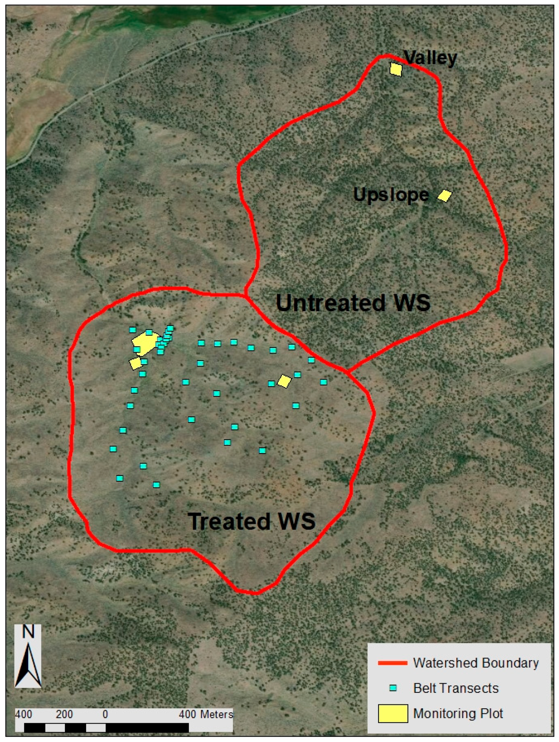
41]. The study site includes two watersheds (WS): an untreated WS (96 hectares) and a treated WS (116 hectares) (
Figure 1). During 2005 to 2006, nearly 90% of western juniper trees were removed from the treated WS. Trees were cut using chainsaws, the boles were removed, and tree limbs were scattered [
42].
Climate in central Oregon is semiarid and precipitation falls largely during the fall and winter months. Average annual precipitation (2009–2017) at the study site is 358 mm [
41]. Elevation at the study site ranges from 1350 to 1500 m. The orientation of the treated WS is primarily north by northwest while the untreated WS is largely oriented toward the north [
43]. The average slope is 25% in the untreated WS and 24% in the treated WS [
43].
Overstory vegetation at the treated WS is dominated by big sagebrush, while western juniper is the dominant species at the untreated WS. Understory vegetation in both watersheds is dominated by perennial grasses, primarily bluebunch wheatgrass [
Pseudoroegneria spicata (Pursh.) Á. Löve], Idaho fescue (
Festuca idahoensis Elmer), Indian ricegrass [
Achnatherum hymenoides (Roem. and Schult.) Barkworth], Sandberg bluegrass (
Poa secunda J. Presl), and Thurber’s needlegrass [
Achnatherum thurberianum (Piper) Barkworth] and some annual grasses, such as cheatgrass (
Bromus tectorum L.) [
43,
44]. As reported by Ray et al. [
44], juniper canopy cover at the untreated WS is 31% and at the treated WS is less than 1%, this based on surveys in 2015. According to the juniper occupancy classification described by Miller et al. [
2], the untreated WS is considered at the highest level, Phase III, in which juniper is at nearly 30% occupancy and it is the dominant overstory species.
2.2. Vegetation Measurements
We calculated juniper-sapling population density, canopy cover, and age characteristics at the watershed scale in the treated WS, and adult and sapling-stage tree density and canopy cover at the plot scale in both watersheds.
At the watershed scale, we installed 41 belt transects (30 m by 3 m) to measure juniper-sapling count, height, and crown width in the treated WS. The belt transects were located across the landscape to represent varying aspect and slope characteristics. A subsample of 18 saplings representing common tree characteristics (i.e., height and width) observed in the treated WS were removed to determine tree age using techniques described by Phipps [
45].
At the plot scale, we installed two 2000 m
2 monitoring plots in each watershed. One plot was installed in a valley location near the watershed outlet and one in an upstream location (
Figure 1). In the untreated WS, tree canopy cover was estimated using a spherical concave densiometer (model A) (Forestry Suppliers, Jackson, MS, USA) across five 40 m parallel transects in each plot. Tree canopy cover was measured every 5 m, facing each cardinal direction, in each 40 m transect. The two plots in the untreated WS were also used to assess juniper canopy cover estimates using UAV-based imagery. All juniper (sapling and adult stages) were counted on the ground to determine tree population density in the monitoring plots at both watersheds. No adult-stage trees were present in either of the two plots in the treated WS; therefore, we only measured sapling count in each 2000 m
2 plot.
An 11,600 m
2 plot in the treated WS (
Figure 1) was employed to assess juniper sapling estimates obtained using the various UAV-based methods described below. A subset of juniper saplings in the larger plot were selected to assess the accuracy of juniper identification.
2.3. Unmanned Aerial Vehicle (UAV)-Based Imagery Collection and Analysis
We collected UAV-based imagery from multiple low elevation (40 to 50 m) flights conducted on 21 June 2018, 15 and 16 July 2018, and 12 October 2018. In order to minimize shadows, flights occurred around noon and early afternoon. Aside from temperature, weather conditions at the time of each flight were similar with scattered clouds present and light, variable winds. Data collected in October 2018 and in the summer of 2018 were used to compare multispectral imagery results across seasons in the treated WS. Three quadcopter UAV (
Table 1) were used to collect data. Multispectral imagery (red, green, blue, near-infrared, and red-edge) was captured using a RedEdge camera (MicaSense, Inc., Seattle, WA, USA). The RedEdge camera was attached either to a Matrice 100 (DJI, Shenzhen, China) or to a Solo (3D Robotics, Inc., Berkeley, CA, USA) UAV for multispectral imagery collection. RGB (red, green, and blue wavelengths) imagery was collected using a DJI Phantom 3 Professional camera (DJI, Shenzhen, China). The Phantom 3 was not used for image collection at the treated WS, the red, green, and blue bands were extracted from the multispectral raster and used for analysis of visual imagery instead.
These quadcopter UAV were selected for use as they provide a flexible platform that can be adapted for multiple types of data collection. Additionally, given the remote location and lack of suitable launching and landing areas, a fixed wing aircraft would be difficult to use. The quadcopters used in this study offer the advantage of being relatively easy to operate, making them an ideal candidate to be used by land managers who may not have flight experience or access to more expensive UAV.
Flight plans were created and conducted using the Pix4Dcapture (Pix4D SA, Lausanne, Switzerland) mobile application, or flown manually. Relatively low flight altitudes (40 to 50 m above ground level) were employed in order to assess the ability of the UAV-imagery to detect juniper saplings. These flight altitudes were chosen as they provide relatively high spatial resolution, while requiring less flight time than much lower flight altitudes. While time requirements for UAV-based data collection were not intensive (flights averaged less than 12 min), the intent of this study was to assess a method that could be applied to larger study areas in the future. Additionally, the height of mature juniper in the untreated WS required a minimum of 40 m flight altitude to ensure sufficient clearance from the top of the trees. An overlapping grid pattern was flown to ensure minimum 80% forward overlap and 60% side overlap. Sufficient overlap was confirmed using the PhotoScan professional (Agisoft LLC, St Petersburg, Russia) program after individual images were added and aligned. All images were captured at nadir.
Orthomosaics created using RGB imagery had slightly higher spatial resolution than those created using the multispectral imagery. Spatial resolution of the visual band orthomosaic at the untreated valley site was 2.09 cm pixel−1 and 2.02 cm pixel−1 at the untreated upstream site. Spatial resolution of the multispectral imagery at the untreated WS valley site was 3.15 cm pixel−1 and 2.74 cm pixel−1 at the untreated WS upstream site. For the multispectral imagery captured in July 2018 at the treated WS study plot, the orthomosaic was 3.00 cm pixel−1. The orthomosaic created from imagery captured in October of 2018 had a spatial resolution of 2.40 cm pixel−1.
Image processing, including the creation of orthomosaics, was conducted using PhotoScan professional (Agisoft LLC, St Petersburg, Russia). Photo alignment was performed using the highest accuracy setting, with a key point limit of 120,000 and a tie point limit of 30,000. Adaptive camera fitting was performed during this step. To create the dense cloud, the ultra-high quality setting with aggressive depth filtering was used. A mesh was created using the 2.5D height field for surface data with a high face count, using the sparse cloud. The mosaic blending mode was used to build the texture. The dense cloud was used to build the tiled model and digital elevation model (DEM). Orthomosaics were subsequently produced in PhotoScan using the created DEM. Areas with poor image quality and without sufficient overlap (on the edges of the orthomosaic) were excluded from analysis. Image analysis was conducted using ArcGIS (version 10.6, Redlands, CA, USA). No radiometric correction was performed; therefore, brightness numbers were used for image analysis. Georeferencing and alignment of images was performed in ArcGIS using landscape features (e.g., gully intersection points) and selected ground control reference markers with known latitude and longitude positions that could be easily identified in imagery.
2.4. Comparative Analysis, Ground Data versus UAV Imagery
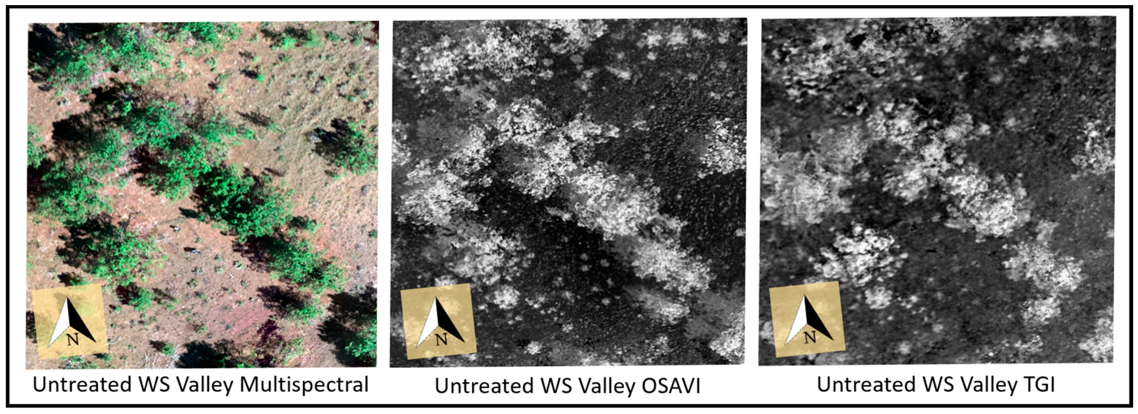
RGB imagery (red, green, and blue wavelengths) and multispectral imagery (red, green, blue, near-infrared, and red-edge wavelengths) were used to assess canopy cover and vegetation cover characteristics. Four vegetation indices were selected to assess canopy cover characteristics of the untreated study plots (
Table 2). As RGB cameras are often more accessible and affordable compared to cameras that capture multispectral imagery, we assessed the effectiveness of using RGB imagery for measuring canopy cover (both mature juniper and juniper saplings), vegetation cover, and juniper identification.
In order to measure canopy cover, the triangular greenness index (TGI) [
46], which indicates chlorophyll content, was applied to the visual imagery at the untreated WS. Additionally, three vegetation indices (NDVI, OSAVI, and TRVI) that utilize multispectral imagery were used in estimating canopy cover at the untreated WS. Vegetation indices were calculated using the Raster Calculator function in ArcGIS, which created a raster of one band with these values.
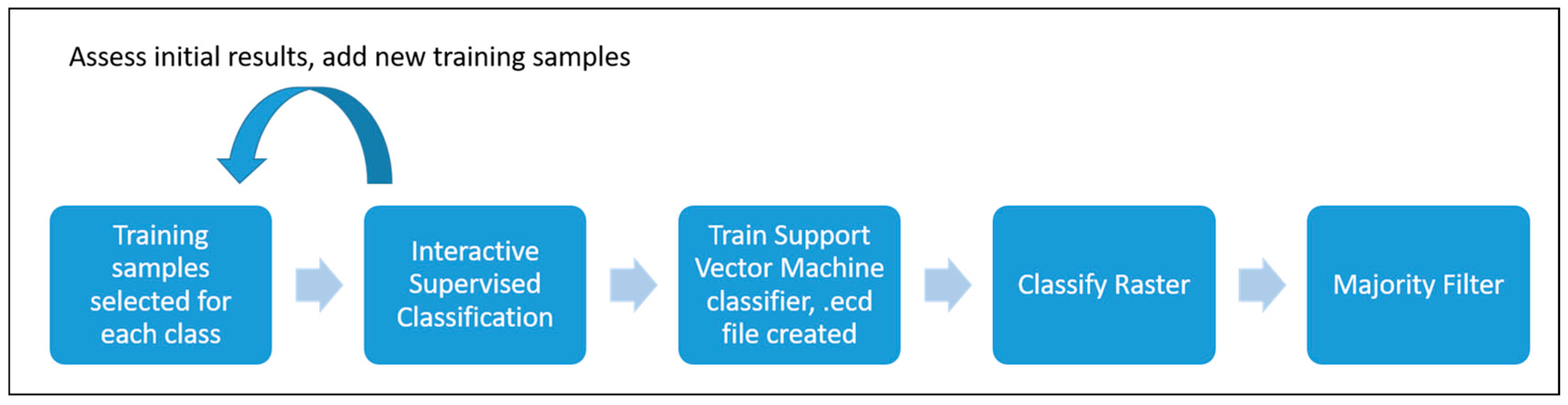
Support vector machine (SVM) supervised classification was also used to assess canopy cover in the untreated WS. RGB imagery (red, green, and blue wavelengths) and multispectral imagery (red, green, blue, near-infrared, and red-edge wavelengths) were used for classification. Using the Training Sample Manager within ArcGIS, polygons were drawn around representative samples of juniper, bare soil, and woody debris. Training sites were selected from different areas of the image to represent the range of reflectance characteristics of each class. An initial image was created using the Interactive Supervised Classification function in order to determine how well the land cover was represented and to determine if more training samples were needed. Once each class was differentiated, the training samples were saved and used for classification. The Train Support Vector Machine Classifier tool in ArcGIS was used to create an Esri Classifier Definition (.ecd) file for each orthomosaic. Using the .ecd file, each the Classify Raster tool was used to perform classification on each raster. In order to minimize noise within the image, and remove small isolated clusters of pixels, the Majority Filter was then applied. The general supervised classification procedure used in this research is shown in
Figure 2.
A pixel-based analysis was conducted to assess juniper density and canopy cover, and total vegetation cover. By determining the number of pixels that correspond to vegetation compared to all other types of ground cover, the percentage of vegetation and canopy cover can be estimated within a given area. For the indices selected in this research, higher values (above 0) corresponded to greater photosynthetic activity or chlorophyll depending on the index applied. For instance, values for NDVI can range from −1 to 1, with areas of bare soil corresponding to values of approximately 0.025 or less, grasslands and shrub vegetation corresponding to values of around 0.09, and areas of dense vegetation corresponding to values of 0.4 or greater [
47]. These values can vary depending on study site characteristics, vegetation type, season, sensor type and calibration, and weather conditions [
48]. Based on visual inspection of the imagery (specifically examining values associated with bare ground, juniper canopy, woody debris, and shadows), threshold values were established for each index to separate vegetation from all other ground cover. The number of pixels with values greater than the threshold were divided by the total number of pixels in order calculate the percent of canopy cover or area covered by vegetation, similar to methods described by Wu [
32].
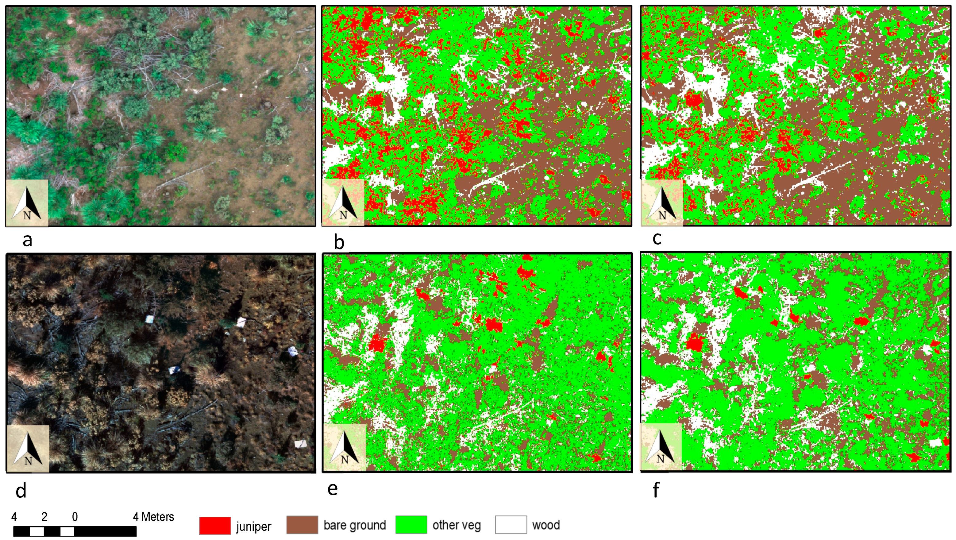
Juniper identification, juniper sapling canopy cover, and vegetation ground cover in the treated WS were assessed for two dates, July 2018 and October 2018. Support vector machine supervised classification was applied to RGB imagery, multispectral imagery (red, green, blue, NIR, and red- edge bands) and imagery with multispectral bands and NDVI values at the treated WS. The same supervised classification process described above was used in the treated WS; however, training samples in the treated WS were divided into four main categories: juniper, other vegetation, woody debris, and bare ground.
The number of pixels classified as juniper, other vegetation, bare ground, or woody debris was tabulated. Similar to calculations made for canopy cover in the untreated plots, the number of pixels represented by each class was divided by the total number of pixels to determine a percent cover of each class in the treated WS. This was then compared to estimates of juniper sapling density and vegetated ground cover calculated using the belt transect method and to the results found using line-point intercept surveys conducted in 2018 at this study site [
49].
To assess the accuracy of the supervised classification in the treated WS, 249 random points were selected in each orthomosaic using the ArcGIS random point tool (one random point corresponded to a board used as a ground control point and was subsequently excluded from this analysis). Additionally, 67 pixels corresponding to juniper saplings were identified within the image and used to assess the accuracy of juniper detection specifically. For accuracy analysis, four main classes were utilized: juniper, other vegetation, woody debris, and bare ground. No assessment was made of the accuracy of detecting specific vegetation species other than western juniper. A confusion matrix was created for each orthomosaic in the treated WS. From the confusion matrix, the user’s accuracy (indication of Type I error), producer’s accuracy (indication of Type II error), Cohen’s kappa coefficient, and overall method accuracy were calculated.


