Article

Spatial-Temporal Patterns of Spruce Budworm Defoliation within Plots in Québec

Faculty of Forestry and Environmental Management, University of New Brunswick, P.O. Box 4400, Fredericton, NB E3B 5A3, Canada
*
Author to whom correspondence should be addressed.
Forests 2019, 10(3), 232; https://doi.org/10.3390/f10030232
Submission received: 24 January 2019 / Revised: 27 February 2019 / Accepted: 1 March 2019 / Published: 6 March 2019
(This article belongs to the Special Issue Protection Strategy against Spruce Budworm)

Abstract

:
We investigated the spatial-temporal patterns of spruce budworm (Choristoneura fumiferana (Clem.); SBW) defoliation within 57 plots over 5 years during the current SBW outbreak in Québec. Although spatial-temporal variability of SBW defoliation has been studied at several scales, the spatial dependence between individual defoliated trees within a plot has not been quantified, and effects of defoliation level of neighboring trees have not been addressed. We used spatial autocorrelation analyses to determine patterns of defoliation of trees (clustered, dispersed, or random) for plots and for individual trees. From 28% to 47% of plots had significantly clustered defoliation during the 5 years. Plots with clustered defoliation generally had higher mean defoliation per plot and higher deviation of defoliation. At the individual-tree-level, we determined ‘hot spot trees’ (highly defoliated trees surrounded by other highly defoliated trees) and ‘cold spot trees’ (lightly defoliated trees surrounded by other lightly defoliated trees) within each plot using local Getis-Ord Gi* analysis. Results revealed that 11 to 27 plots had hot spot trees and 27% to 64% of them had mean defoliation <25%, while plots with 75% to 100% defoliation had either cold spot trees or non-significant spots, which suggested that whether defoliation was high or low enough to be a hot or cold spot depended on the defoliation level of the entire plot. We fitted individual-tree balsam fir defoliation regression models as a function of plot and surrounding tree characteristics (using search radii of 3–5 m). The best model contained plot average balsam fir defoliation and subject tree basal area, and these two variables explained 80% of the variance, which was 2% to 5% higher than the variability explained by the neighboring tree defoliation, over the 3–5 m search radii tested. We concluded that plot-level defoliation and basal area were adequate for modeling individual tree defoliation, and although clustering of defoliation was evident, larger plots were needed to determine the optimum neighborhood radius for predicting defoliation on an individual. Spatial autocorrelation analysis can serve as an objective way to quantify such ecological patterns.

1. Introduction

With advances in spatial analysis theory and methodologies, biologists and ecologists have become more interested in analyzing ecological processes from a spatial point of view. Spatial point pattern analyses can indicate how individuals locate with respect to each other, by testing the complete spatial randomness null hypothesis [1]. Spatial autocorrelation analyses and indices can be applied to detect if the observed value of a variable at one site is dependent on values at neighboring sites [2,3]. The first law of geography states “Everything is related to everything else, but near things are more related than those distant ones” [4]. Spatial autocorrelation analyses are used for ecological processes that are distance-related, including speciation, extinction, dispersal, and synchronous population fluctuations [5,6]. Quantitative indices of spatial autocorrelation identify and characterize distribution patterns of objects of interest on the ground, and help to bridge the gap between mechanisms and the behavior of the investigated phenomenon [7,8]. Therefore, spatial autocorrelation analyses are an appropriate method to detect spatial patterns of insects’ behavior or of forest dynamics related to insect infestations (e.g., [7,8]).
Spruce budworm (Choristoneura fumiferana (Clem.); SBW) outbreaks are a dominant, periodic natural disturbance in eastern Canada [9]. SBW larvae consume the new foliage of balsam fir (Abies balsamea (L.) Mill.) and spruce (Picea spp. A. Dietr.) trees [10], often for 10 or more years. This results in tree mortality typically ranging from about 40% to 85%, depending upon defoliation severity, tree species, and tree age [11,12]. Baskerville and MacLean [13] observed that SBW-caused tree mortality in immature balsam fir tended to have a strongly contagious spatial distribution. Mortality ranged from 18% to 80% of the total volume per hectare, and tended to occur in distinct patches spreading over time, with almost all trees in these patches killed [13]. Variation in mortality from plot to plot was therefore related to the extent to which such patches occurred in each plot. Spatial variability of mortality has important implications for study of stand vulnerability to SBW attack. If within-stand variability is high and apparently not related to stand characteristics [13], then conventional large scale, between-stand, sampling to establish characteristics of vulnerability could lead to statistically significant relationships between mortality and average stand conditions, even when mortality is not functionally related to average conditions [13].
SBW-caused tree mortality is strongly related to cumulative defoliation [14,15,16], so one might assume that a clustered spatial distribution of dead trees reflects higher annual defoliation in those trees than in surrounding trees. No studies have determined spatial patterns of SBW defoliation among trees, so in this study, we used spatial autocorrelation analyses to determine patterns of tree locations (clustered, dispersed, or random) and of annual defoliation of trees for 5 years in 57 plots in Gaspé, Québec, Canada. In addition to implications on stand vulnerability to insect-caused mortality, spatial pattern of defoliation is important for projecting effects on stand growth reduction and mortality in distance-dependent or tree-list growth models (e.g., [17]). Relationships between tree mortality and defoliation are non-linear, so use of average defoliation when some trees actually sustain higher or lower levels of defoliation will underestimate or overestimate impacts. For managing defoliated forests, knowledge of tree-to-tree variability of SBW defoliation can also benefit selection of the scale and methods of biological insecticide spray treatment decisions to target moderate or high infestation.
Although the spatial interrelationships of SBW defoliation levels of trees within a plot is not well understood, intertree variance in defoliation has been observed to be greater than intratree variance or variance between plots in a stand [18]. Defoliation levels are clearly a function of SBW population factors including oviposition site selection, larval and moth dispersal, and larval survival, but also may be influenced by tree, stand, site, and topographical factors. At the landscape scale, studies determining “epicenters” of historical defoliation based on aerial survey data have concluded that host species or volume had only minor effects on defoliation [19,20,21]. Defoliation among plots within stands was typically similar, with low variance (<5%), especially when SBW populations were high, for both eastern [22] and western SBW (Choristoneura occidentalis Freeman; [23]). At finer scales, variation of defoliation of branches within a stand was less than that of shoots on a branch [18], because branches from one site tended to have similar defoliation, and distribution of shoot defoliation tended to follow skewed Poisson distributions at both light and severe defoliation levels. Different host species suffer different degrees of defoliation: white spruce (Picea glauca (Moench) Voss), red spruce (Picea rubens Sarg.), and black spruce (Picea mariana (Mill.) B.S.P.) had approximately 72%, 41%, and 28% as much defoliation as balsam fir [10]. Non-host species also influence defoliation: balsam fir defoliation was lower when hardwood content increased, thought to be because of greater diversity and populations of SBW parasitoids [24,25]. In mixed fir-spruce stands, the density of balsam fir increased SBW defoliation severity in fir-dominated and fir-spruce mixed stands, while density of black spruce decreased the infestation in such stands [26].
There are several possible SBW population-related causes contributing to variable defoliation patterns. The frequency distribution of SBW larvae per tree is positively skewed, with a small proportion of trees hosting populations higher than the average [27]. This could result from unequal attraction of female moths to host trees, perhaps based on strength of their stimulus to the olfactory responses of the insect [27], or different exposure to light [28]. In stands without severe defoliation, SBW egg populations were usually higher on taller and dominant trees that were well exposed to light, while in severely defoliated stands, greater defoliation of exposed trees makes them less attractive to female moths, and correlation between the egg population and tree height became negative [27,28]. Larval SBW populations were greater in upper crowns because female moths tended to deposit eggs on the peripheral shoots of the crown [28,29]. Early instar larval dispersal may cause redistribution of larval population within a stand, but mass dispersal movements only occur in severely infested stands where food supply becomes exhausted [27]; such larval dispersal is risky because of high resulting mortality [30]. Although no direct data exist on between-tree spatial distributions of SBW egg masses or larval populations, spatial clustering of other insects has been observed: both adult and larval cereal leaf beetle (Oulema melanopus (L.)) were in a clustered distribution within 0.4 hectare areas in wheat fields [31]; and emerald ash borer (Agrilus planipennis) larval populations declined with distance, with about 90% of larvae within 100 m of adults’ emergence sites [32].
In this study, we evaluated spatial patterns of 5 years of individual-tree SBW defoliation within 57 plots in Québec. Objectives were to: (1) determine whether spatial locations of tree stems within plots were clustered, dispersed, or random, as a baseline for comparing defoliation patterns; (2) quantify spatial aggregation of defoliation within plots, and detect if there was spatial dependence of individual tree defoliation; and (3) test whether the defoliation level of an individual balsam fir tree can be predicted using plot, tree, and neighboring tree defoliation and other characteristics. We evaluated two predictions: (1) defoliation of individual trees within a plot may be spatially clustered in some cases, i.e., highly defoliated trees will be surrounded by highly defoliated trees, and vice versa for lightly defoliated, as would result from preferential selection of oviposition sites by female moths; and (2) defoliation of an individual balsam fir tree within a plot can be predicted using defoliation level and species composition of surrounding neighborhood trees, combined with plot-level defoliation and species composition.

2. Materials and Methods

2.1. Study Area and Data Collection

The study area was located in the central Gaspé Peninsula region of Québec, a balsam fir-white birch (Betula papyrifera Marsh.) mixed eco-district [33]. According to aerial forest surveys, light SBW defoliation began in 2012 or 2013 and increased to moderate or severe levels since 2014 [34]. The 57 circular (400 m2) study plots were established in 2014, with 19 plots about 15 km northwest of Amqui and 38 plots about 40 km southwest of Causapscal. These are a subset of plots studied by Donovan et al. [35] and Zhang et al. [25], and additional description of the sites is available there. Plot locations are shown in Figure 1 of [35]. However, we have omitted 15 plots that were harvested from 2016 to 2018, and three plots missing some defoliation data in 2015. A portion of our studied plots were protected by aerial spraying of Bacillus thuringiensis biological insecticide to control defoliation each year: 28% of plots in 2014, 42% in 2015, 30% in 2016, 26% in 2017, and 38% in 2018. The plots included a total of 3693 trees, of which 3200 were balsam fir or spruce.
Plot center coordinates were recorded using survey-grade GPS. Attribute data collected for each tree with diameter at breast height (DBH) ≥10 cm included species, tree azimuth, distance from plot center, DBH, total tree height, height of the live crown base, crown widths in north, east, south, and west directions, and annual ocular estimates of current defoliation using binoculars. Foliage defoliation was classified into seven classes: 0%–10%, 11%–20%, 21%–40%, 41%–60%, 61%–80%, 81%–99%, and 100%, and the midpoint of each class was used for calculations. To calibrate observers and check accuracy, one mid-crown branch was sampled from each of 8 to 15 trees per host species per plot (sample sizes based on [36]), and defoliation of each of 25 current-year shoots was assessed using the same classes as for ocular defoliation. Defoliation data were collected after SBW feeding ceased each year from 2014 to 2018. Criteria for plot selection and methods of data collection were described in more detail in [35].

2.2. Point Pattern Analyses

We first evaluated whether tree stems within plots were clustered, dispersed, or randomly distributed using a point pattern analysis of average nearest neighborhoods [37]. Liu [38] reviewed five methods for spatial pattern analysis, and indicated that when the purpose is to analyze the nearest neighbor, Pielou’s statistics [39] and Clark and Evans’ statistics (used in this study; [40]) perform the best in avoiding Type II errors, although there was evidence showing that Pielou’s statistics [39] have more power for detecting regular and Poisson cluster patterns. The Clark and Evans’ statistics calculate the ratio of mean observed distance between all trees and their nearest neighbors, and expected mean nearest neighbor distance for a random arrangement [40]:
R = D O D E
where D O = i = 1 n d i n is the observed mean distance between each tree and its nearest neighbor, in which d i equals the distance between tree i and its nearest neighbor, and n is the number of trees in the plot; D E = 0.5 n A is the expected mean distance between each tree and its nearest neighbor given in an ideal random pattern, in which A is the area of minimum enclosing rectangle around all features (set as plot area, 400 m2, in this study). Generally, if the average distance is less than the average for a hypothetical random distribution (R < 1), the distribution is considered to be clustered; if R > 1, the distribution tends to be dispersed, and if R = 1 the distribution follows a random arrangement. The standard deviation, z-score was calculated as [40]:
z = D 0 D E S E
where S E = 0.26136 n 2 A is the standard error of the mean, in which the constant is derived from the radius of a circle of unit area and the Poisson probability model. Average nearest neighborhood analyses were done separately on each of the 57 plots, on all host trees, by species (balsam fir, black spruce, and white spruce), and on hardwood trees. Analyses were only applied when number of trees analyzed was ≥5 per plot.

2.3. Spatial Autocorrelation Analyses

Two quantitative indices were used to detect and characterize spatial patterns of defoliation at plot and tree levels. First, global Moran’s I coefficient [41] was computed, to produce an overall measure of similarities or dissimilarities between neighboring trees within a plot. It helps to estimate the intensity of spatial dependence for the entire plot and summarizes it with a single value [1,42]. Global Moran’s I was calculated as:
I =   n S 0 · W i j Z i Z j Z i 2
where W i j is the spatial weight between tree i and tree j using an inverse distance weighting method to conceptualize the spatial relationships between trees, such that numerical weights quantified the proximity of pair-wise observations, with closer trees having higher spatial weights [2]. Z i or Z j is the deviation of defoliation for tree i or tree j from the mean of all trees in the plot, calculated as x i x ¯ or x j x ¯ ; S 0 = i = 1 n   j = 1 n W i j is the aggregate of all spatial weights and n is the number of trees in the plot. Global Moran’s I ranges from −1 to 1; I > 0 or I < 0 corresponds to a positive or negative spatial correlation, representing spatial clustering or spatial dispersal, respectively, and I = 0 means a random distribution [3]. However, global Moran’s I is difficult to interpret unless combined with statistical significance tests, and can only be interpreted within the context of the complete spatial randomness hypothesis. Z-score for global Moran’s I was computed as [41]:
Z = I E ( I ) V ( I )
where E ( I ) = 1 n 1 is the expectation of global Moran’s I under the complete spatial randomness hypothesis; when the sample size tends to be infinite, E ( I ) is zero. V ( I ) is the variance, computed as V ( I ) = E ( I 2 ) ( E ( I ) ) 2 . The analyses omitted cases when all trees in the plot had the same level of defoliation.
Following the global Moran’s I analysis, Getis-Ord Gi* analysis, which is a local spatial autocorrelation statistic, was used to determine defoliation patterns of individual trees within each plot. Getis-Ord Gi* analysis tests the spatial clustering of high or low values of the measured variable around location i , characterizing the internal clustering within each plot by determining the extent to which defoliation of a given tree is surrounded by a cluster of trees with either high or low values [43,44]. Gi* statistics proportionally compare the local sum for tree i and its neighbors to the sum of all trees, which is computed as [43]:
G i * = j W i j x j X ¯ j W i j S n j W i j 2 ( j W i j ) 2 n 1
where i is the subject tree, x j is the defoliation value for one of the neighboring trees j , W i j is the spatial weight between subject tree i and neighboring tree j determined by the fixed distance band method (i.e., neighboring trees within 5 m were set with the same weight), X ¯ is the average defoliation value of the entire plot, n is the total number of trees in the plot, and S is the standard deviation of the entire plot, given by S = j = 1 n x j 2 n ( X ¯ ) 2 . Gi* is calculated as sum of the differences between individual values and the mean of all individuals. Therefore, Gi* is a standard normal distribution z-score. A statistically significant Gi* results when the difference between calculated local sum and expected local sum is too large to be a random chance. High and positive values of Gi* indicate ‘hot spot trees’, severely defoliated trees that are surrounded by severely defoliated trees, whereas low and negative values indicate ‘cold spot trees’, lightly defoliated trees surrounded by lightly defoliated trees.
Both size and shape of the study plot affect the ability of the Gi* statistics to accurately estimate the type and significance of a spatial pattern, because objects near the edge would have fewer neighbors than those in the middle of the plot. This is known as edge effect [45]. If the plot does not contain the entire spatial process under study, as was the case in this research, it is important to consider edge effects to increase stability and power of statistics resulting from sampling [46]. In this study, to avoid complicated edge-correcting procedures [47], we used an inner buffer zone in each plot to compensate for edge effects. A search radius of 5 m was used, and a corresponding central circular subplot of 6 m was selected inside each plot. Trees in the border area were excluded from the Getis-Ord Gi* analysis. All spatial autocorrelation analyses were done using ArcMap 10.4 (ESRI, Redlands, CA, USA).
Both global Moran’s I and local Getis-Ord Gi* spatial autocorrelation analyses were conducted separately on each of the 57 sample plots, and results of these and point-pattern tree location analyses were presented as the number and percentage of plots that had significantly clustered results. With such a wide range of defoliation conditions purposefully sampled across plots and years (ranging from <5% to >90% current annual defoliation), it was highly unlikely that there would be a single clustered or not clustered answer for all plots.

2.4. Tree Defoliation Regression Model

To determine whether defoliation levels of individual balsam fir can be predicted by plot or surrounding-tree characteristics, nonlinear mixed effect regression models were fitted, with plots nested within years as random effects. Current-year defoliation of balsam fir was the response variable. Plot-level predictors included average defoliation and % basal area of each host species and hardwoods per plot. Tree-level predictors included basal area of the subject balsam fir, defoliation of the subject balsam fir in the previous year, average defoliation of surrounding (3, 4, and 5 m search radii) trees (calculated for balsam fir, black spruce, white spruce, and for all host trees), total basal area of surrounding trees (balsam fir, hardwood, spruce trees, and for all host trees), total basal area of surrounding trees with basal area higher than the subject balsam fir, representing relative social status of the subject tree (calculated for balsam fir, spruce, and for all host trees). Defoliation of the subject balsam fir in the previous year acted as a temporal variable, and those neighborhood-related predictors at the tree level acted as spatial variables because they represented defoliation levels and species composition around the subject tree. We also considered the possible impact of insecticide spraying by including a dummy variable representing the subject balsam fir being sprayed or not in the corresponding year. All subject trees were balsam fir located in the central 6 m radius subplots, and effects were tested using surrounding 3, 4, or 5 m search radii with at least one neighbor in the neighborhood.
Gradient boosting is a machine learning technique, which identifies the performance of decision trees by using gradients in the loss function (i.e., a measurement of the goodness of coefficients in the model) in a sequential fashion [48]. Gradient Boosting Machine analysis [49] was used to determine the most important variables using the “caret” package [50] within R [51]. One of the important features of Gradient Boosting Machine analysis is variable importance, which was summarized as the ranked variables based on their relative influence (importance) in training the model. Relative influence was computed based on how often a variable was selected for splitting, weighted by the squared improvement to the model in each split [52]. Basal area of the subject tree was included in each tested model because it is related to foliage amount and to avoid having zero variance of fitted individual balsam fir defoliation values within a plot when it was predicted solely using plot-level variables. Except for the subject tree basal area, relatively important predictors were added into candidate models in sequence according to their ranks by Gradient Boosting Machine analysis. The contribution of newly-added predictors was determined by likelihood ratio tests, and based on this, whether the models should include the added predictors was evaluated. Highly correlated variables (r ≥ 0.7) were avoided in the candidate models. Beta regression was used because the response variable, defoliation of the subject balsam fir, was constrained between 0 and 1 (0% to 100%). A logit-link function was used to set up linear relationships between the response and predictor variables. Likelihood ratio tests were also used to determine whether the random effects from plots or years were significant, by comparing a mixed effect model and a fixed effect model as a null model. The significance of individual predictors in the models was assessed by t tests. The “nlme” and “gnls” functions in the “nlme” package [53] were used in fitting mixed effect models and fixed effect models, respectively.
Assumptions of normality and homoscedasticity of residuals were evaluated using residual plots. Goodness of fit of candidate models was assessed and compared by root mean square error (RMSE), adjusted r2, and mean bias (predicted-observed).

3. Results

3.1. Stand and Plot Characteristics

Characteristics of the 57 plots in the sampled stands ranged from 13.5 to 18.0 m height, 14.9 to 22.2 cm DBH, 1075 to 1919 stem ha−1 density, and 34.9 to 47.7 m2 ha−1 basal area (Table 1). Basal area of each host species in the stands was 6% to 98% balsam fir, 0% to 70% black spruce, and 0% to 65% white spruce (Table 1). Plot species composition averaged 64% balsam fir, 19% black spruce, 10% white spruce, 2% other softwood species, and 5% hardwood species (Table 1). Annual defoliation in the 5 years from 2014 to 2018 averaged 34%, 51%, 28%, 38%, and 32% by ocular estimation, and 45%, 52%, 34%, 54%, and 38% by shoot defoliation estimation on sampled branches. Plot locations were specifically selected in 2014 to represent the full range of defoliation from <10% to 90%–100%, and insecticide sprayed plots were the only way to obtain low defoliation levels.

3.2. Spatial Patterns of Tree Stems within Plots

Average nearest neighborhood analyses for all host species within each plot showed that 35 plots (61%) had randomly distributed host trees, and the remaining 22 plots (39%) had significantly dispersed host trees (α = 0.05; Table 2). No plots had significantly clustered host tree stem locations. The average nearest neighborhood analysis for each host species and hardwoods also showed that balsam fir, black spruce, white spruce, and hardwoods were distributed randomly or dispersed in most plots, and few (0% to 5%) plots had significantly clustered tree stems by species (Table 2). Generally, the null hypothesis that there is no difference between observed and random nearest neighbor values was not rejected for almost all plots, either by species or for all host species combined. The results of these average nearest neighborhood analyses set the baseline tree spatial distributions for the following spatial autocorrelation analyses of defoliation levels.

3.3. Spatial Patterns of Current Year Defoliation for Plots

Global Moran’s I analyses results for all host species showed that each year from 2014 to 2018, 47%, 28%, 35%, 30%, and 33% of plots, respectively, had significantly clustered intertree defoliation patterns (α = 0.05; Table 3). This indicates that in these plots, defoliated trees had a strong tendency to be located closer to trees with similar defoliation values. These results therefore differed substantially from that for the spatial locations of trees, in which no plots had clustered tree spatial distributions (Table 2). In roughly one-third to one-half of the plot-years, defoliation of trees was clustered. A total of 45 plots (79%) exhibited clustered defoliation in at least one of the five sampled years. For balsam fir, 11% to 33% of plots had clustered defoliation distribution, somewhat fewer than for all host species combined (Table 3). With relatively few spruce present, only 2% to 5% and 0% to 4% of plots had clustered defoliation on black spruce and white spruce (Table 1 and Table 3). A dispersed defoliation pattern occurred only for black spruce in one plot, with no dispersed defoliation patterns for all host trees or by species.
We used box plots to compare the distributions of total basal area, average annual plot defoliation, and standard deviation of individual tree defoliation between plots with clustered and non-clustered defoliation on all host trees (Figure 1). Plots were divided into 25% balsam fir plot basal area classes (x-axis) in Figure 1 because the analyzed plots varied widely in species composition. With low balsam fir content (<25% basal area), 18 plot-years with non-clustered defoliation had significantly higher basal area than 12 plot-years with clustered defoliation (mean 46 versus 41 m2 ha−1; Figure 1a). Overall, annual plot defoliation levels increased with the proportion of balsam fir in plots (Figure 1b). Plots with clustered defoliation had higher defoliation in all balsam fir % basal area classes than plots with non-clustered defoliation, significantly different for 50% to 75% basal area fir plots (43% versus 33% defoliation in clustered and non-clustered plots; Figure 1b). Plots with clustered defoliation consistently had higher standard deviations of tree defoliation than plots with non-clustered defoliation, with significant differences of 9.1% and 6.4% defoliation for plots with 0% to 25% and 50% to 75% balsam fir (Figure 1c).

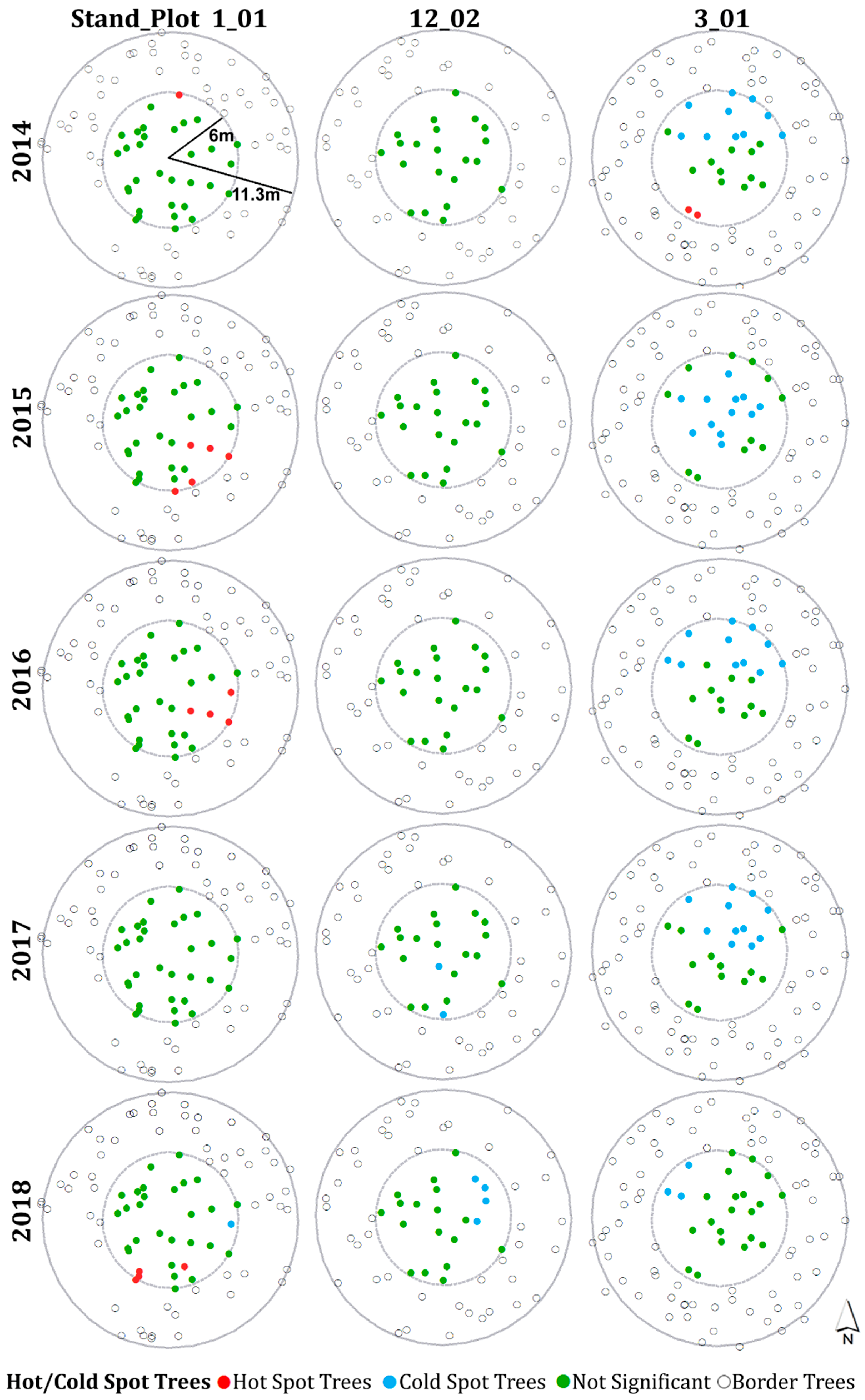
3.4. Hot Spot and Cold Spot Trees within Plots

In Figure 2, we integrated results of the global Moran’s I and Getis-Ord Gi* statistics for all analyzed plots in all years. We ordered the stand_plot number by annual plot defoliation each year, in order to visually convey that although defoliation was clustered in some plots (shown by * above each bar), how and whether hot or cold spots could be detected showed a tendency to be related to defoliation level. Hot spot trees (red bars in Figure 2) tended to be in lightly defoliated plots, and cold spot trees (blue bars) tended to be in highly defoliated plots. Across the five sampled years, minimum 42 and maximum 80 hot spot trees (highly defoliated trees surrounded by other highly defoliated trees), and minimum 44 and maximum 59 cold spot trees (lightly defoliated trees surrounded by other lightly defoliated trees) were detected within the 6 m-radius subplots (Figure 2). Plots with hot or cold spot trees did not necessarily have clustered defoliation (* in Figure 2), although plots with significantly clustered defoliation did tend to have hot or cold spot trees: 25%–45%, 10%–31%, 13%–35%, and 10%–36% of plots with clustered defoliation had hot spot trees, cold spot trees, both hot and cold spot trees, and non-significant spots, respectively, across the five years (Figure 2).
There was a tendency for highly defoliated plots to have more cold spot trees, and lightly defoliated plots to have more hot spot trees (Figure 2). Over the five sampled years, plots with 0%–25% defoliation had 0–4 cold spots (0.3 on average) and 0–8 hot spots (1.0 on average), while plots with 75%–100% defoliation had 0–12 cold spots (1.7 on average) and virtually no hot spots. Over the 5 sampled years, 27, 11, 26, 18, and 26 plots had hot spot trees (including those with both hot and cold spot trees), while 13 (48%), 7 (64%), 16 (62%), 7 (39%), and 7 (27%) of them were 0%–25% defoliated (Figure 3). Plots with 75%–100% defoliation had either cold spot trees or non-significant spots within them, except one plot in 2017 with >75% defoliation that had one hot spot tree (Figure 3d). That plot experienced 75% annual defoliation, with 100% balsam fir composition, and had only one balsam fir detected as a hot spot tree in 2017.
Stem maps of three example plots were selected to represent generally low, moderate, and high defoliation that had hot and cold spot trees (Figure 4 and Figure 5). Plot 1_01 had low defoliation (5%–17%) in all years from 2014 to 2018 (Figure 4), and had 1–5 hot spot trees in four years, but none in 2017 (Figure 5). Interestingly, locations of hot spot trees were the same for only three of the 11 trees, in two years (2015–2016); otherwise they differed. Mean defoliation of trees in plot 12_02 ranged from 29% to 74% over the five years, and covered defoliation classes from 0%–20% to 81%–100% (Figure 4). There were no hot spot trees and only six cold spot trees in two years in this plot (Figure 5). Plot 3_01 had very high defoliation (85%) in three years, and moderate (31% and 52%) defoliation in 2014 and 2018 (Figure 4), resulting in many cold spot trees in all years and two hot spot trees in the first year only (Figure 5). It is noteworthy that at moderate defoliation levels, variation among trees was high: with 31% mean defoliation in 2018 in plot 3_01, trees with all five 20% defoliation classes occurred in the plot (Figure 4).

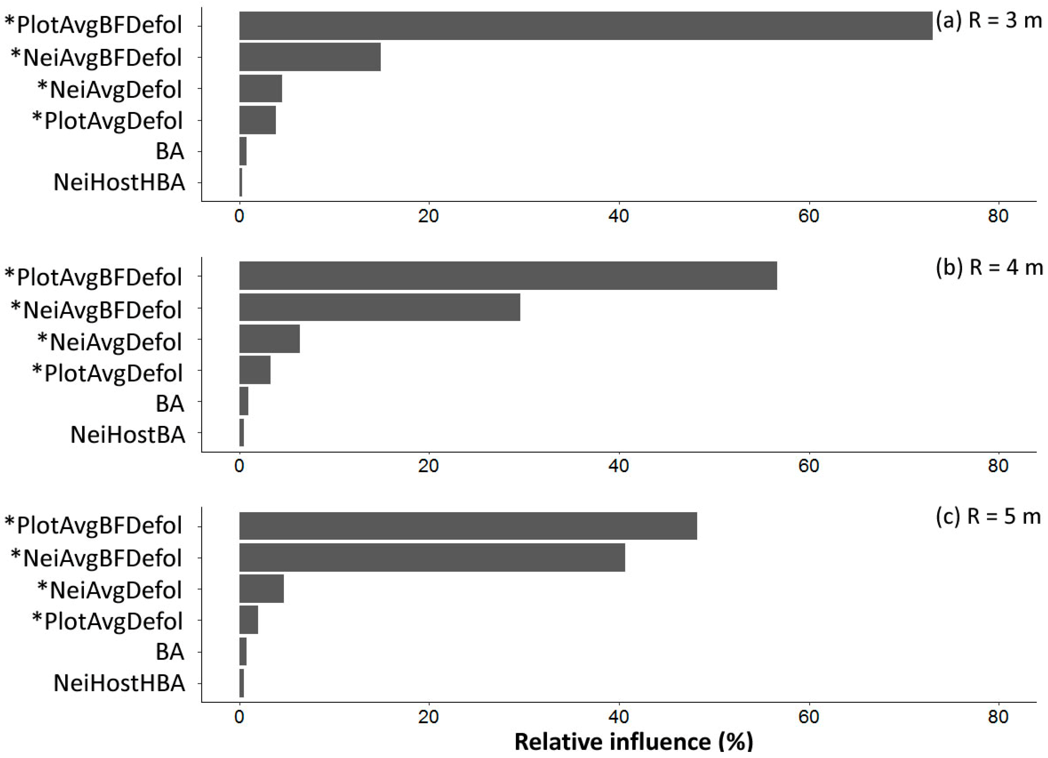
3.5. Prediction of Subject Tree Balsam Fir Defoliation Using Regression Models

Results of Gradient Boosting Machine analysis consistently showed that plot average annual defoliation of balsam fir was the most important predictor for all three neighborhood search radii, with relative influence of 73%, 57%, and 48% for 3, 4, and 5 m search radii, respectively (Figure 6). Given the variability in defoliation among trees within a plot (e.g., Figure 4), it was surprising to us that plot average defoliation was superior to local within-plot defoliation for the three radii circles in predicting defoliation of a single tree. Average annual defoliation of surrounding balsam fir had the highest relative influence of all tree-level predictors, at 15%, 30%, and 41% for 3, 4, and 5 m search radii (Figure 6). Table 4 lists all plot- and tree-level predictors investigated using Gradient Boosting Machine analysis. Correlation analysis of the predictor variables suggested that plot average balsam fir defoliation (i.e., mean of all trees in the plot) was highly correlated (r > 0.9) with average defoliation of balsam fir within its neighborhood (i.e., within 3, 4, or 5 m circles). Therefore, average defoliation of balsam fir at the plot and tree level were not both included in the same candidate model. Basal area, representing subject tree size, was included in each model. Total basal area of host trees having higher basal area than the subject tree within 3 and 5 m, and total basal area of host trees within 4 m, which ranked as the sixth most important predictors, were also tested in candidate models. Spraying and defoliation in the previous year variables had little influence (0.3% at most) in the Gradient Boosting Machine analysis. The remaining predictors, including spray and defoliation in the previous year, were dropped in the following process.
Plots nested within years was added as a random effect variable, but likelihood ratio tests suggested that it had little influence, in comparing models with mixed effects versus fixed effects as a null model (p = 0.9). This meant that the variance associated with plot-nested-in-year groups could occur by chance. Therefore, the random effects were removed from candidate models, and fit statistics of models with only fixed effects were reported (Table 5).
Results of models to predict subject tree defoliation as a function of plot and neighboring tree variables showed that Model 1 based on plot average balsam fir defoliation and subject tree basal area explained 80% of the total variance in the response variable, with RMSE of 14.1% and bias of 2.8% (Table 5). Variance explained by plot average balsam fir defoliation was slightly higher than that explained by neighboring average balsam fir defoliation within 4 or 5 m (79% and 78%), which were higher than 3 m (75%; Table 5). Coefficients (p < 0.01) in these four candidate models (Models 1, 2, 4, and 6) were all positive, indicating that higher subject balsam fir defoliation occurred with higher subject tree basal area, higher plot average defoliation, and higher neighboring balsam fir average defoliation. The other two predictors, total basal area of host trees having higher basal area than the subject tree within 3 m (Model 3) and total basal area of host trees within 4 m (Model 5) were significant (p < 0.05), and had slightly better r2, RMSE, and bias, compared to Model 1. This suggested that including neighboring host tree basal area can slightly improve performance compared to a model that including only plot average balsam fir defoliation.

4. Discussion

4.1. Is Defoliation of Individual Trees Clustered

Generally, defoliation was clustered in some plots and some years, depending on defoliation levels. Plots with clustered defoliation consistently had higher annual defoliation than plots with non-clustered defoliation. Spatial locations of fir and spruce trees within plots were randomly distributed in 61% of plots and dispersed in the remaining 39% of plots; none were clustered. In contrast, an average of 35% of plots had significantly clustered defoliation distributions of balsam fir and spruce, with amount clustered varying from 28% to 47% among years. Plots with clustered defoliation had larger standard deviation of defoliation among trees, reflecting higher variability in defoliation within the plots.
The added value of this study is the first demonstration that there can be spatially clustered defoliation patterns among trees, even though the baseline tree locations are not spatially clustered. Although SBW populations on each tree were not measured, higher defoliation must result from higher SBW populations or higher larval survival. Clustered defoliation within plots probably results from SBW population processes, primarily moth oviposition selection and larval dispersal. SBW egg populations are usually higher on taller and dominant trees that are well exposed to light, but severe defoliation may make such trees less attractive to female moths, and the correlation between egg population and tree height becomes negative [27,28]. Larval dispersal leads to tree-to-tree redistribution of SBW, which can result in reduced tree-to-tree correlation (i.e., more even SBW pressure), because such dispersal occurs rather randomly in direction especially at a small scale [29]. Not much air movement is needed for larval dispersal due to their light body weight [54]. However, a large proportion of the SBW population must be engaged in dispersal processes to contribute to a noticeable change in intertree population distribution, and such mass movements only occur in highly defoliated stands with high competition among feeding larvae [27]. Additionally, SBW larvae tend to avoid risky dispersal behavior because of the high probability of mortality during dispersal [30]. Given that current annual defoliation exceeded 80% in only 8.5% of our 260 plot-years sampled (and most of those were in 2015), larval dispersal probably had minor effects on intertree defoliation distribution in this study.

4.2. Interpretation of Local Hot and Cold Spot Trees

Conceptually, Getis-Ord Gi* is the ratio of average local defoliation over average global (plot in our case) defoliation. It indicates hot spot (highly defoliated trees surrounded by other highly defoliated) and cold spot (lightly defoliated trees surrounded by other lightly defoliated) trees. Over all plots and years, 28% of plot-years had hot spot trees, 18% had cold spot trees, 12% had both, and 42% had none; in other words, there was significant spatial variability in defoliation in 58% of cases. Whether defoliation is high enough to be a hot spot or low enough to be a cold spot depends on the general defoliation level of the plot. SBW outbreak spatial-temporal dynamics typically begin with patchy low-level but increasing defoliation for several years, observable on individual branches initially and then on trees. It typically takes several years for SBW populations to build sufficiently to result in widespread severe defoliation (>70% of current year foliage on most trees) across stands and regions. Defoliation is most variable among trees and plots at moderate (30%–70% of current year foliage) levels; when low or very high, defoliation tends to be consistent [18]. Plots with severe defoliation tended to have cold spot trees, and plots with light defoliation tended to have hot spot trees. This is because a target highly defoliated tree surrounded by other highly defoliated trees will have a higher value of Gi* (ratio of average local defoliation over average global defoliation) if it is located in a plot with overall low defoliation, while it is more likely to be non-significant if it is located in a highly defoliated plot. A similar principle applies for cold spot trees.
Highly significant global spatial autocorrelation can lead to overly liberal local spatial autocorrelation, which means significance tests of the local-spatial-autocorrelation coefficients can reject the null hypothesis excessively when a global spatial autocorrelation occurs [42]. Although the local spatial statistic used in this study, Getis-Ord Gi*, does not need extra significant tests, values are still sensitive to the overall spatial structure of defoliation in plots [1]. Other statistics have been proposed to address such issues [55,56], but a local statistic avoiding influence from or accounting for global spatial autocorrelation is still needed [57]. As suggested by Sokal et al. [42], the major application of local spatial autocorrelation tests should be exploratory instead of significance testing. Our main conclusion here is that in about one-third to one-half of plots over 5 years, clustered defoliation patterns occurred, at either higher (hot spot) or lower (cold spot) levels than the plot average. Therefore the spatially contagious SBW-caused tree mortality observed by Baskerville and MacLean [13] within a uniform immature balsam fir stand, occurring at a scale smaller than the 400 m2 plots, may have resulted from higher defoliation in some trees. Over the longer term, mortality creating such ‘holes’ in stands is also probably exacerbated by windthrow disturbance [58,59].

4.3. Prediction of Subject Balsam Fir Defoliation

Average defoliation for the full plot combined with subject tree basal area explained 80% of the variability of subject balsam fir defoliation, which was 2% to 5% higher than the variability explained by the neighboring tree defoliation, over the 3, 4, and 5 m search radii tested. However, the relative influence of neighboring tree defoliation on subject tree defoliation increased as search radius increased, from 15% to 30% to 41% as search radius increased from 3 m to 4 m to 5 m. At a 5 m search radius, the relative influence of neighboring tree defoliation was nearly as high as plot average defoliation. This suggested that a neighborhood search radius larger than 5 m, and therefore larger overall plot size, was needed, and it might be superior to average plot defoliation for individual-tree-defoliation prediction.
There was wide variation in defoliation among trees in the sampled plots, and although plot mean defoliation was the strongest predictor of subject tree defoliation, inferring similar average defoliation levels for all trees in a plot creates a problem when inputting defoliation values into stand growth models to predict effects of defoliation on growth and mortality. Model driving relationships between growth reduction, mortality, and defoliation are non-linear, such that trees with the highest defoliation will sustain substantially higher rates of growth reduction and mortality than the mean. Recognizing that a portion of trees are in hot or cold spots, with clusters of higher or lower defoliation, implies that model predictions will be more accurate using input distributions of defoliation for tree-list models and spatial defoliation distributions for distance-dependent growth models.
For these primarily balsam fir plots, species composition at either the plot level or tree level was not a meaningful predictor of individual balsam fir defoliation. The stands sampled had 51%–98% fir in all but four plots, which had 77%–92% black and white spruce. The four spruce plots exhibited hot and cold spot trees in 75% of the 20 plot-years sampled. Although hardwood content has been shown to influence SBW defoliation [24,25], hardwoods comprised only an average of 6% of basal area in these plots (range 1%–20%). This gave too few samples to test neighborhood effects of hardwoods on defoliation. Although insecticide spraying was an important predictor when forecasting plot-level annual defoliation [35], it had little impact on tree-level annual defoliation in this study, because the effects of spraying were already reflected by the plot mean defoliation variable. Defoliation of subject trees in the previous year also showed little influence, suggesting that individual-tree defoliation can vary considerably from year to year, as a function of SBW population level each year and insecticide treatments.

5. Conclusions

We evaluated neighborhood effects on individual-tree SBW defoliation, including the detection of defoliation clustering by spatial autocorrelation analysis, and the prediction of subject balsam fir defoliation by mixed effect regression. Key messages from the results include:
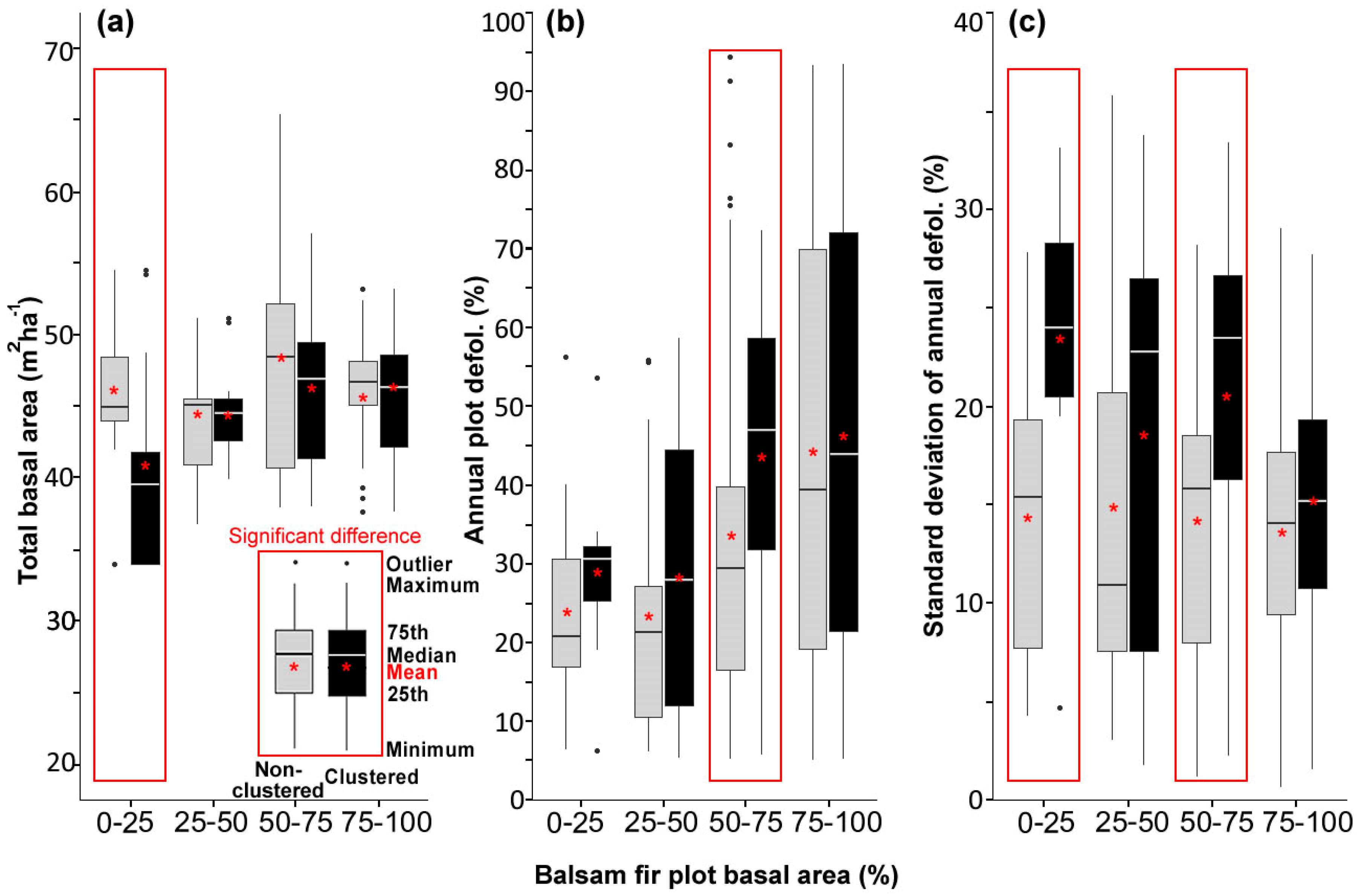
  • Including all host species, 47%, 28%, 35%, 30%, and 33% of plots showed significantly clustered defoliation patterns from 2014 to 2018. Plots with clustered defoliation tended to have higher and less uniform defoliation among trees. Results suggested that spatial defoliation patterns resulted from uneven SBW pressure on trees, perhaps from oviposition site selection.
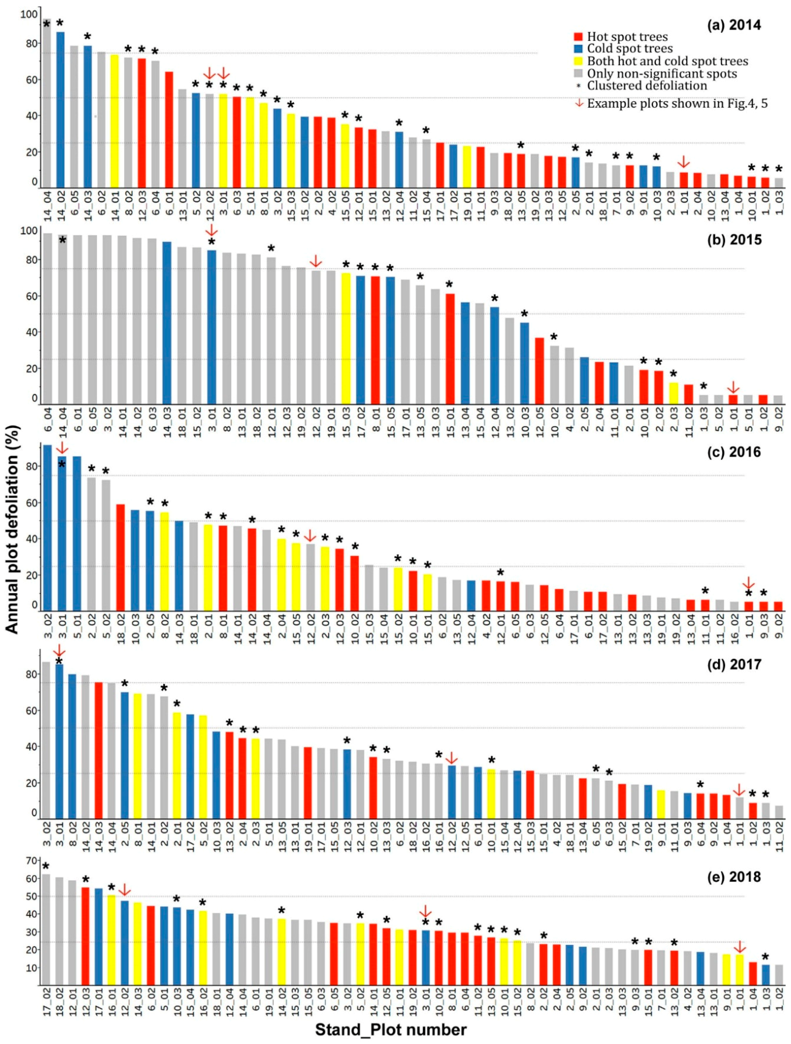
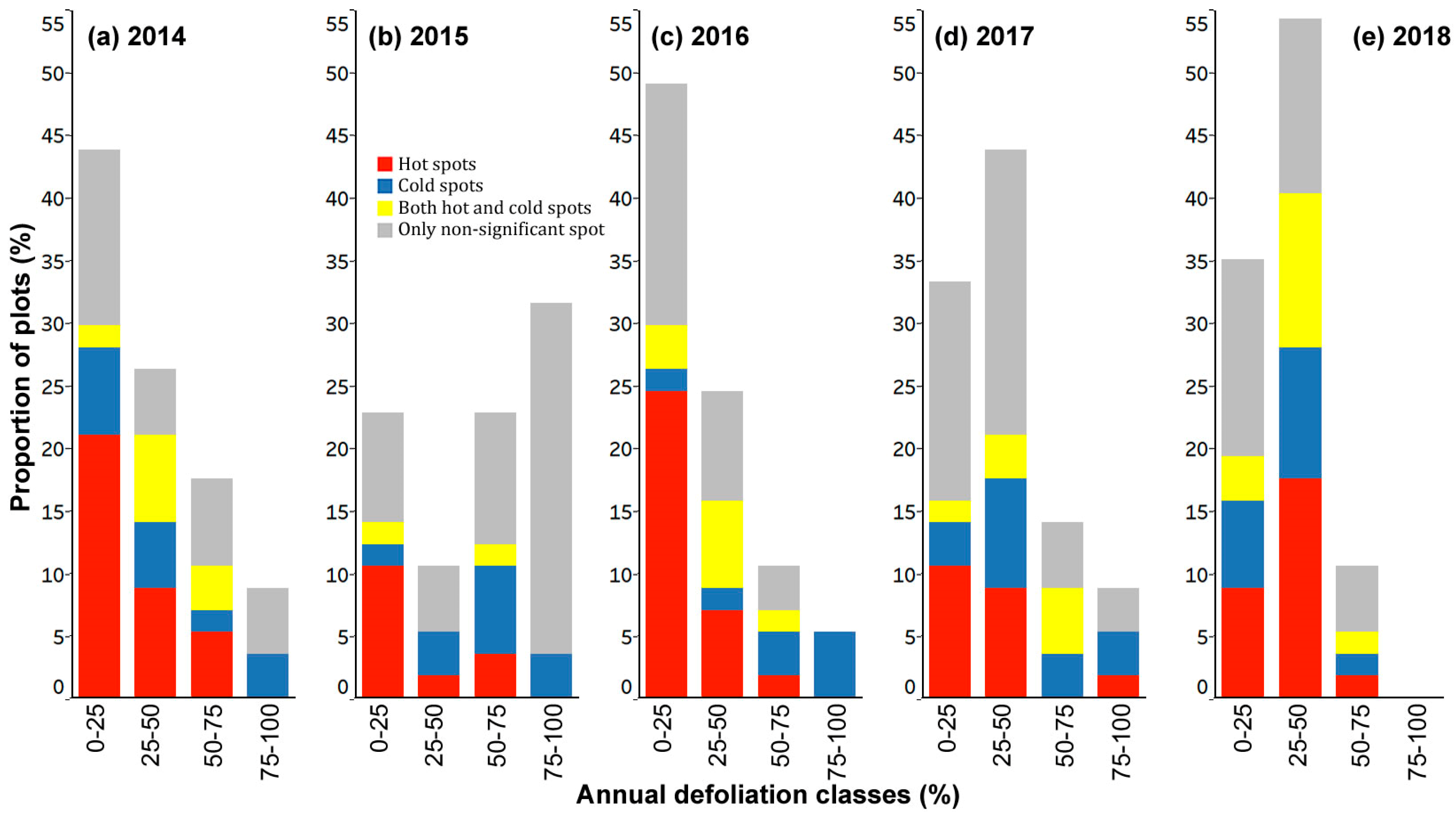
  • Plots with severe defoliation generally tended to exhibit cold spot trees, and plots with light defoliation tended to have hot spot trees, because whether defoliation was high or low enough to be a hot or cold spot depended on the defoliation level of the entire plot.
  • Plot-level average defoliation combined with subject tree basal area explained 80% of the variability of subject balsam fir defoliation, which was 2% to 5% higher than variability explained by the neighboring tree defoliation.
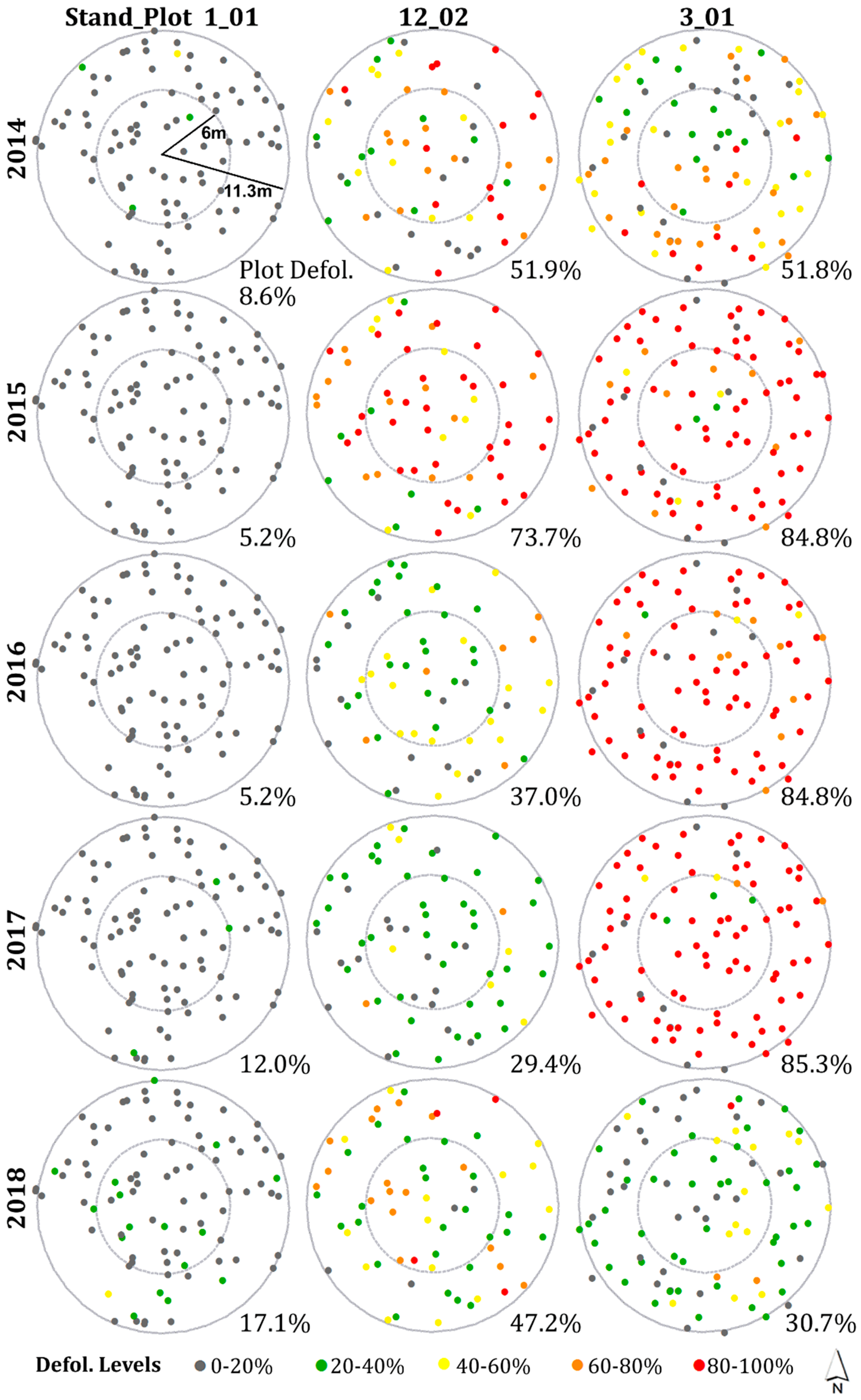
  • Spatial variability of defoliation decreased with larger radius neighborhoods from 3 to 5 m, suggesting that a neighborhood search radius larger than 5 m (and thus plot sizes larger than 400 m2 (11.3 m radius) to deal with edge effects) may provide better predictions of subject balsam fir defoliation.
  • For these primarily balsam fir plots, species composition at both plot and tree levels were not significant predictors of individual balsam fir defoliation.
Spatial autocorrelation analysis is a useful means to describe and quantify spatial-temporal, ecological patterns of insect defoliation. For managing defoliated forests, knowledge of tree-to-tree variability of SBW defoliation can benefit selection of the scale and methods of biological insecticide spray treatment decisions to target moderate or high infestation. Our results showed that in spite of within-plot variability, there was far more plot-to-plot variability in defoliation. It indicated that a large number of plots is preferred rather than fewer larger plots. On the other hand, understanding spatial variability among defoliation levels of trees can help improve defoliation inputs into distance-dependent or tree-list stand growth models (e.g., [17]). If only the averaged plot defoliation is used as inputs to growth and yield models for all trees in a stand, it will underestimate growth reduction, and especially mortality for those trees suffering from higher defoliation levels (i.e., clusters). Adopting a distribution of defoliation levels of trees as model inputs rather than merely the plot average values would likely result in more accurate forecasts of SBW impacts.

Author Contributions

The authors provided equal contribution towards decisions regarding methodology and study design. M.L. wrote the manuscript draft; D.A.M., C.R.H., and J.O. contributed to manuscript revision and development.

Funding

This research was funded by the Atlantic Innovation Fund project “Spruce Budworm Early Intervention Strategy”, grant number 203544 to D.A.M. The Atlantic Innovation Fund was funded by the Atlantic Canada Opportunities Agency.

Acknowledgments

We acknowledge project support from the Healthy Forest Partnership. We appreciate the excellent work of all field assistants involved in the data collection: Shawn Donovan, Sean Lamb, Rebecca Landry, Bo Zhang, Maggie Brewer, Jessica Cormier, Olivia Doran, David Alton, and Kerrstin Trainor.

Conflicts of Interest

The authors declare no conflict of interest.

References

  1. Dale, M.R.; Fortin, M.J. Spatial Analysis: A Guide for Ecologists; Cambridge University Press: Cambridge, UK, 2014. [Google Scholar]
  2. Sokal, R.R.; Oden, N.L. Spatial autocorrelation in biology 1. Methodology. Biol. J. Linn. Soc. 1977, 10, 199–228. [Google Scholar] [CrossRef]
  3. Cliff, A.D.; Ord, J.K. Spatial Processes: Models & Applications; Pion Ltd.: London, UK, 1981. [Google Scholar]
  4. Tobler, W.R. A computer movie simulating urban growth in the Detroit region. Geogr. Econ. 1970, 46, 234–240. [Google Scholar] [CrossRef]
  5. Augustin, N.H.; Mugglestone, M.A.; Buckland, S.T. The role of simulation in modelling spatially correlated data. Environmetrics 1998, 9, 175–796. [Google Scholar] [CrossRef]
  6. Knapp, R.A.; Matthews, K.R.; Preisler, H.K.; Jellison, R. Developing probabilistic models to predict amphibian site occupancy in a patchy landscape. Ecol. Appl. 2003, 13, 1069–1082. [Google Scholar] [CrossRef]
  7. Ryan, P.A.; Lyons, S.A.; Alsemgeest, D.; Thomas, P.; Kay, B.H. Spatial statistical analysis of adult mosquito (Diptera: Culicidae) counts: An example using light trap data, in Redland Shire, southeastern Queensland, Australia. J. Med. Entomol. 2004, 41, 1143–1156. [Google Scholar] [CrossRef] [PubMed]
  8. Foster, J.R.; Townsend, P.A.; Mladenoff, D.J. Spatial dynamics of a gypsy moth defoliation outbreak and dependence on habitat characteristics. Landsc. Ecol. 2013, 28, 1307–1320. [Google Scholar] [CrossRef]
  9. Hardy, Y.; Mainville, M.; Schmitt, D.M. Spruce Budworms Handbook: An Atlas of Spruce Budworm Defoliation in Eastern North America, 1938–1980; U.S. Department of Agriculture, Forest Service, Cooperative State Research Service: Washington, DC, USA, 1986.
  10. Hennigar, C.R.; MacLean, D.A.; Quiring, D.T.; Kershaw, J.A. Differences in spruce budworm defoliation among balsam fir and white, red, and black spruce. For. Sci. 2008, 54, 158–166. [Google Scholar]
  11. MacLean, D.A. Vulnerability of fir-spruce stands during uncontrolled spruce budworm outbreaks: A review and discussion. For. Chron. 1980, 56, 213–221. [Google Scholar] [CrossRef]
  12. MacLean, D.A. Effects of spruce budworm outbreaks on the productivity and stability of balsam fir forests. For. Chron. 1984, 60, 273–279. [Google Scholar] [CrossRef]
  13. Baskerville, G.L.; MacLean, D.A. Budworm-Caused Mortality and 20-Year Recovery in Immature Balsam fir Stands; Inf. Rep. M-X-102; Maritimes Forest Research Centre, Canadian Forestry Service: Fredericton, NB, Canada, 1979; p. 56.
  14. MacLean, D.A.; Ostaff, D.P. Patterns of balsam fir mortality caused by an uncontrolled spruce budworm outbreak. Can. J. For. Res. 1989, 19, 1087–1095. [Google Scholar] [CrossRef]
  15. Erdle, T.A.; MacLean, D.A. Stand growth model calibration for use in forest pest impact assessment. For. Chron. 1999, 75, 141–152. [Google Scholar] [CrossRef] [Green Version]
  16. Chen, C.; Weiskittel, A.; Bataineh, M.; MacLean, D.A. Even low levels of spruce budworm defoliation affect mortality and ingrowth but net growth is more driven by competition. Can. J. For. Res. 2017, 47, 1546–1556. [Google Scholar] [CrossRef]
  17. Lamb, S.M.; MacLean, D.A.; Hennigar, C.R.; Pitt, D.G. Forecasting forest inventory using imputed tree lists for LiDAR grid cells and a tree-list growth model. Forests 2018, 9, 167. [Google Scholar] [CrossRef]
  18. MacLean, D.A.; Lidstone, R.G. Defoliation by spruce budworm: Estimation by ocular and shoot-count methods and variability among branches, trees, and stands. Can. J. For. Res. 1982, 12, 582–594. [Google Scholar] [CrossRef]
  19. Hardy, Y.J.; Lafond, A.; Hamel, L. The epidemiology of the current spruce budworm outbreak in Quebec. For. Sci. 1983, 29, 715–725. [Google Scholar]
  20. Gray, D.R.; MacKinnon, W.E. Outbreak patterns of the spruce budworm and their impacts in Canada. For. Chron. 2006, 82, 550–561. [Google Scholar] [CrossRef] [Green Version]
  21. Zhao, K.; MacLean, D.A.; Hennigar, C.R. Spatial variability of spruce budworm defoliation at different scales. For. Ecol. Manag. 2014, 328, 10–19. [Google Scholar] [CrossRef]
  22. Ostaff, D.P.; MacLean, D.A. Spruce budworm populations, defoliation, and changes in stand condition during an uncontrolled spruce budworm outbreak on Cape Breton Island, Nova Scotia. Can. J. For. Res. 1989, 19, 1077–1086. [Google Scholar] [CrossRef]
  23. Alfaro, R.I.; Shore, T.L.; Wegwitz, E. Defoliation and mortality caused by western spruce budworm: Variability in a Douglas-fir stand. J. Entomol. Soc. 1984, 81, 33–38. [Google Scholar]
  24. Su, Q.; MacLean, D.A.; Needham, T.D. The influence of hardwood content on balsam fir defoliation by spruce budworm. Can. J. For. Res. 1996, 26, 1620–1628. [Google Scholar] [CrossRef]
  25. Zhang, B.; Maclean, D.A.; Johns, R.C.; Eveleigh, E.S. Effects of hardwood content on balsam fir defoliation during the building phase of a spruce budworm outbreak. Forests 2018, 9, 530. [Google Scholar] [CrossRef]
  26. Bognounou, F.; Grandpre, L.D.; Pureswaran, D.S.; Kneeshaw, D. Temporal variation in plant neighborhood effects on the defoliation of primary and secondary hosts by an insect pest. Ecosphere 2017, 8, 1–15. [Google Scholar] [CrossRef]
  27. Morris, R.F.; Mott, D.G. Dispersal and the spruce budworm. In The Dynamics of Epidemic Spruce Budworm Populations; Morris, R.F., Ed.; Memoirs of the Entomological Society of Canada: Ottawa, ON, Canada, 1963; Volume 95, pp. 180–189. [Google Scholar]
  28. Morris, R.F. The development of sampling techniques for forest insect defoliators, with particular reference to the spruce budworm. Can. J. Zool. 1955, 33, 107–223. [Google Scholar] [CrossRef]
  29. Beckwith, R.C.; Burnell, D.G. Spring larval dispersal of the western spruce budworm (Lepidoptera: Tortricidae) in north-central Washington. Environ. Entomol. 1982, 11, 828–832. [Google Scholar] [CrossRef]
  30. Miller, C.A. The measurement of spruce budworm populations and mortality during the first and second larval instars. Can. J. Zool. 1958, 36, 409–422. [Google Scholar] [CrossRef]
  31. Reay-Jones, F.P.F. Spatial distribution of the cereal leaf beetle (Coleoptera: Chrysomelidae) in wheat. Environ. Entomol. 2010, 39, 1943–1952. [Google Scholar] [CrossRef] [PubMed]
  32. Mercader, R.J.; Siegert, N.W.; Liebhold, A.M.; Mccullough, D.G. Dispersal of the emerald ash borer, Agrilus planipennis, in newly-colonized sites. Agric. For. Entomol. 2009, 11, 421–424. [Google Scholar] [CrossRef]
  33. Bélanger, L.; Bergeron, Y.; Camiré, C. Ecological Land Survey in Quebec. For. Chron. 1992, 68, 42–52. [Google Scholar] [CrossRef]
  34. QMRNF: Québec Ministère des Ressources Naturelles et de la Faune. Aires Infestées par la Tordeuse des Bourgeons de l’épinette au Québec en 2014. Available online: http://www.mffp.gouv.qc.ca/publications/forets/fimaq/insectes/tordeuse/TBE_2014_P.pdf (accessed on 20 October 2017).
  35. Donovan, S.D.; MacLean, D.A.; Kershaw, J.A.; Lavigne, M.B. Quantification of forest canopy changes caused by spruce budworm defoliation using digital hemispherical imagery. Agric. For. Meteorol. 2018, 262, 89–99. [Google Scholar] [CrossRef]
  36. MacLean, D.A.; MacKinnon, W.E. Sample sizes required to estimate defoliation of spruce and balsam fir caused by spruce budworm accurately. North. J. Appl. For. 1998, 15, 135–140. [Google Scholar]
  37. Ebdon, D. Statistics in Geography: A Practical Approach; Basil Blackwell Ltd.: New York, NY, USA, 1985. [Google Scholar]
  38. Liu, C. A comparison of five distance-based methods for spatial pattern analysis. J. Veg. Sci. 2001, 12, 411–416. [Google Scholar] [CrossRef]
  39. Pielou, E.C. The use of point-to-plant distances in the study of the pattern of plant populations. J. Ecol. 1959, 47, 607–613. [Google Scholar] [CrossRef]
  40. Clark, P.J.; Evans, F.C. Distance to nearest neighbor as a measure of spatial relationships in populations. Ecol. Soc. Am. 1954, 35, 445–453. [Google Scholar] [CrossRef]
  41. Moran, P.A.P. Notes on continuous stochastic phenomena. Biometrika 1950, 37, 17–23. [Google Scholar] [CrossRef] [PubMed]
  42. Sokal, R.R.S.; Oden, N.L.; Thomson, B.A. Local spatial autocorrelation in biological variables. Biol. J. Linn. Soc. 1998, 65, 41–62. [Google Scholar] [CrossRef] [Green Version]
  43. Getis, A.; Ord, J.K. The analysis of spatial association by use of distance statistics. Geogr. Anal. 1992, 24, 189–206. [Google Scholar] [CrossRef]
  44. Ord, J.K.; Getis, A. Local spatial autocorrelation statistics: Distributional issues and an application. Geogr. Anal. 1995, 27, 286–305. [Google Scholar] [CrossRef]
  45. Monserud, R.A.; Ek, A.R. Plot edge bias in forest stand growth simulation models. Can. J. For. Res. 1974, 4, 419–423. [Google Scholar] [CrossRef]
  46. Sui, D.Z.; Hugill, P.J. A GIS-based spatial analysis on neighborhood effects and voter turn-out: A case study in College Station, Texas. Polit. Geogr. 2002, 21, 159–173. [Google Scholar] [CrossRef]
  47. Ripley, B.D. Tests of “randomness” for spatial point patterns. J. R. Stat. Soc. 1979, 41, 368–374. [Google Scholar] [CrossRef]
  48. Friedman, J.H. Greedy function approximation: A gradient boosting machine. Ann. Stat. 2001, 29, 1189–1232. [Google Scholar] [CrossRef]
  49. Ridgeway, G. Generalized boosted models: A guide to the GBM package. R Package Vignette. 2007. [Google Scholar]
  50. Kuhn, M. Building Predictive Models in R Using the caret Package. J. Stat. Softw. 2008, 28, 1–26. [Google Scholar] [CrossRef]
  51. R Core Team. R: A Language and Environment for Statistical Computing; R Foundation for Statistical Computing: Vienna, Austria, 2018. [Google Scholar]
  52. Elith, J.; Leathwick, J.R.; Hastie, T. A working guide to boosted regression trees. J. Anim. Ecol. 2008, 77, 802–813. [Google Scholar] [CrossRef] [PubMed] [Green Version]
  53. Lindstrom, M.J.; Bates, D.M. Nonlinear mixed effects models for repeated measures data. Int. Biom. Soc. 1990, 46, 673–687. [Google Scholar] [CrossRef]
  54. Batzer, H.O. Hibernation site and dispersal of spruce budworm larvae as related to damage of sapling balsam fir. J. Environ. Entomol. 1968, 61, 216–220. [Google Scholar] [CrossRef]
  55. Kabos, S.; Csillag, F. The analysis of spatial association on a regular lattice by join-count statistics without the assumption of first-order homogeneity. Comput. Geosci. 2002, 28, 901–910. [Google Scholar] [CrossRef]
  56. Boots, B. Developing local measures of spatial association for categorical data. J. Geogr. Syst. 2003, 5, 139–160. [Google Scholar] [CrossRef]
  57. Getis, A. A history of the concept of spatial autocorrelation: A geographer’s perspective. Geogr. Anal. 2008, 40, 297–309. [Google Scholar] [CrossRef]
  58. Taylor, S.L.; MacLean, D.A. Spatiotemporal patterns of mortality in declining balsam fir and spruce stands. For. Ecol. Manag. 2007, 253, 188–201. [Google Scholar] [CrossRef]
  59. Taylor, S.L.; MacLean, D.A. Legacy of insect defoliators: Increased wind-related mortality two decades after a spruce budworm outbreak. For. Sci. 2009, 55, 256–267. [Google Scholar]
Figure 1. Comparison of plots with and without significant clustering of defoliation (based on results of global Moran’s I analyses (α = 0.05) for all host trees) by 25% balsam fir plot basal area classes for (a) total basal area in the plot, (b) average current year defoliation, and (c) standard deviation of individual tree defoliation within plots.
Forests 10 00232 g001
Figure 2. Average current year defoliation of plots, ordered from highest to lowest defoliation each year from 2014 to 2018 (ae), showing plots with significantly clustered (α = 0.05) defoliation (*), with hot spot trees (red), cold spot trees (blue), both hot and cold spot trees (yellow), and only non-significant trees (grey), based on results of Getis-Ord Gi* analyses (α = 0.05).
Forests 10 00232 g002
Figure 3. Proportion of plots with hot spot trees, cold spot trees, both hot and cold spot trees, and only non-significant trees (based on results of Getis-Ord Gi* analyses (α = 0.05)) by 25% annual defoliation classes from 2014 to 2018 (ae).
Forests 10 00232 g003
Figure 4. Stem maps of tree locations (diameter at breast height (DBH) ≥ 10 cm) of three example plots for five years, showing spatial distribution of defoliation. The three example plots were selected to represent generally low (1_01), moderate (12_02), and high (3_01) defoliation levels that contained hot spot and cold spot trees (shown in Figure 5).
Forests 10 00232 g004
Figure 5. Stem maps of tree locations shown for the inner 6 m center of three example plots (same as in Figure 4) for five years, showing spatial distribution of hot spot trees, cold spot trees, and non-significant trees (based on results of Getis-Ord Gi* analyses; α = 0.05).
Forests 10 00232 g005
Figure 6. Relative influence (%) of the six most important predictor variables based on Gradient Boosting Machine analysis to predict current year defoliation of individual balsam fir trees (%) with neighborhood tree search radius (R) of (a) 3 m, (b) 4 m, or (c) 5 m. Predictor variable abbreviations are described in Table 4, and predictors marked with * were highly correlated with each other (correlation coefficient r ≥ 0.7).
Forests 10 00232 g006
Table 1. Summary of mean ( X ¯ ) and standard deviation (σ) characteristics per stand of 57 plots located in 19 stands near Amqui and Causapscal, Québec, Canada.
Stand No.No. Plots 1Density (stem ha−1)DBH 2
(cm)
Height
(m)
Basal Area (m2 ha−1)Species Composition 3
(% Basal Area)
X ¯ σ X ¯ σ X ¯ σ X ¯ σBFBSWSHWOSW
14191928915.01.113.70.938.83.85430467
25177541717.01.416.51.042.84.3514233
32191363616.01.416.00.941.86.7831115
411200 20.1 18.0 39.8 627652
52182515915.80.116.10.238.11.7981 1
65160032916.52.214.82.038.74.0777477
711950 14.9 14.8 38.3 78 202
82180015915.80.415.50.638.11.7702056
93180842616.72.616.21.344.24.286 2111
103147527517.20.915.90.536.32.7227071
112123810618.11.016.50.734.91.8544122
125177519117.00.817.31.043.55.7503892
135125031720.01.718.41.142.25.557 412
144184423616.50.816.20.642.44.590 10
155173022416.70.415.20.740.35.3692821
162111317722.21.119.20.247.72.755 432
172107515920.30.916.10.240.02.071 11615
182132526517.50.313.50.644.04.580 20
192176363617.32.914.23.051.38.559 111418
1 We originally (in 2014) established at least three plots per stand [35], but 15 of the original 75 plots were harvested from 2016 to 2018, and three plots had missing defoliation data. Analyses in this paper are all within plots, and stands were used here only to summarize general characteristics. 2 DBH = diameter at breast height. 3 Species abbreviations: BF = balsam fir; BS = black spruce; WS = white spruce; HW = hardwood species, including balsam poplar (Populus balsamifera), American mountain ash (Sorbus americana), trembling aspen (Populus tremuloides), willow (Salix spp.), white birch, yellow birch (Betula alleghaniensis), red maple (Acer rubrum), mountain maple (Acer spicatum), and striped maple (Acer pensylvanicum); OSW = non-host softwood species, including eastern white cedar (Thuja occidentalis), eastern white pine (Pinus strobus), and eastern larch (Larix laricina).
Table 2. Number and percentage of plots with clustered, dispersed, or random tree stem locations based on average nearest neighbor analyses (α = 0.05), for balsam fir, black spruce, white spruce, hardwoods, and all host species per plot.
Balsam FirBlack SpruceWhite SpruceHardwoodsAll Host Species
Clustered01 (2%)03 (5%)0
Dispersed21 (37%)3 (5%)1 (2%)2 (4%)22 (39%)
Random35 (61%)20 (35%)12 (21%)25 (44%)35 (61%)
Table 3. Number and percentage of plots with significantly clustered patterns of defoliation of trees, based on global Moran’s I analyses among years, for balsam fir, black spruce, white spruce, and all host species in each plot (α = 0.05, search radius = 5 m).
YearBalsam FirBlack SpruceWhite SpruceAll Host Species
201419 (33%)1 (2%)2 (4%)27 (47%)
201511 (19%)3 (5%)016 (28%)
201613 (23%)1 (2%)020 (35%)
20176 (11%)2 (4%)017 (30%)
201815 (26%)2 (4%)019 (33%)
Table 4. Abbreviations and description of predictor variables at both plot and tree levels included in Gradient Boosting Machine analysis to determine their relative importance in predicting annual defoliation of a subject balsam fir tree.
Predictor VariablesDescription
Plot level
PlotAvgDefolAverage annual defoliation of all host species per plot (%)
PlotAvgBFDefolAverage annual defoliation of balsam fir per plot (%)
PlotBFBA% basal area of balsam fir
PlotBSBA% basal area of black spruce
PlotWSBA% basal area of white spruce
PlotHWBA% basal area of hardwoods
SprayDummy variable: whether the plot was sprayed by insecticide (1) in corresponding given year or not (0)
Tree level 1
BABasal area of the subject balsam fir (m2 ha−1)
PreYearDefolAnnual defoliation of subject balsam fir in previous year (%)
NeiAvgDefolAverage annual defoliation of neighboring1 host trees (%)
NeiAvgBFDefolAverage annual defoliation of neighboring balsam fir (%)
NeiAvgBSDefolAverage annual defoliation of neighboring black spruce (%)
NeiAvgWSDefolAverage annual defoliation of neighboring white spruce (%)
NeiHostBATotal basal area of neighboring host trees (m2 ha−1)
NeiBFBATotal basal area of neighboring balsam fir (m2 ha−1)
NeiSPBATotal basal area of neighboring spruce trees (m2 ha−1)
NeiHWBATotal basal area of neighboring hardwoods (m2 ha−1)
NeiHBATotal basal area of all trees with basal area greater than the subject balsam fir in the neighborhood (m2 ha−1)
NeiHostHBATotal basal area of host trees with basal area greater than the subject balsam fir in the neighborhood (m2 ha−1)
NeiSPHBATotal basal area of spruce trees with basal area greater than the subject balsam fir in the neighborhood (m2 ha−1)
NeiBFHBATotal basal area of balsam fir with basal area greater than the subject balsam fir in the neighborhood (m2 ha−1)
1 Search radii of 3, 4, and 5 m were used for balsam fir trees in a circular subplot of 6 m inside each plot.
Table 5. Adjusted r2, root mean squared error (RMSE), and mean bias of predictions of individual balsam fir defoliation (%) by candidate models with neighborhood tree search radius equal to 3, 4, and 5 m. Predictor variable abbreviations are described in Table 4.
Candidate ModelsPredictorsFit Statistics 1
Adjusted r2RMSEBias
Model 1PlotAvgBFDefol + BA0.80010.14110.0028
Search radius = 3 m
Model 2NeiAvgBFDefol + BA0.75390.15660.0017
Model 3PlotAvgBFDefol + BA + NeiHostHBA0.80150.14060.0025
Search radius = 4 m
Model 4NeiAvgBFDefol + BA0.78230.14730.0019
Model 5PlotAvgBFDefol + BA + NeiHostBA0.80070.14090.0027
Search radius = 5 m
Model 6NeiAvgBFDefol + BA0.78890.14500.0025
1 The fit statistics were tested for fixed effect models without random effect terms, which in previous model runs had little contribution to models by likelihood ratio tests (p = 0.9).

