Spatial Autocorrelation Analysis of Multi-Scale Damaged Vegetation in the Wenchuan Earthquake-Affected Area, Southwest China

Abstract

Major earthquakes can cause serious vegetation destruction in affected areas. However, little is known about the spatial patterns of damaged vegetation and its influencing factors. Elucidating the main influencing factors and finding out the key vegetation type to reflect spatial patterns of damaged vegetation are of great interest in order to improve the assessment of vegetation loss and the prediction of the spatial distribution of damaged vegetation caused by earthquakes. In this study, we used Moran’s I correlograms to study the spatial autocorrelation of damaged vegetation and its potential driving factors in the nine worst-hit Wenchuan earthquake-affected cities and counties. Both dependent and independent variables showed a positive spatial autocorrelation but with great differences at four aggregation levels (625 × 625 m, 1250 × 1250 m, 2500 × 2500 m, and 5000 × 5000 m). Shrubs can represent the characteristics of all damaged vegetation due to the significant linear relationship between their Moran’s I at the four aggregation levels. Clustering of similar high coverage of damaged vegetation occurred in the study area. The residuals of the standard linear regression model also show a significantly positive autocorrelation, indicating that the standard linear regression model cannot explain all the spatial patterns in damaged vegetation. Spatial autoregressive models without spatially autocorrelated residuals had the better goodness-of-fit to deal with damaged vegetation. The aggregation level 8 × 8 is a scale threshold for spatial autocorrelation. There are other environmental factors affecting vegetation destruction. Our study provides useful information for the countermeasures of vegetation protection and conservation, as well as the prediction of the spatial distribution of damaged vegetation, to improve vegetation restoration in earthquake-affected areas.

1. Introduction

Major earthquakes are geologically disastrous and can trigger serious ecological degradation. In addition to causing massive human casualties, such earthquakes induce vegetation destruction [1], heavy economic losses [2], biodiversity reduction [3], aggravated sedimentation [4], and landscape fragmentation [5]. Ecological restoration in earthquake-affected areas is a slow process due to the unstable, crude, and nutrient-poor soil conditions left in the wake of secondary geo-hazards [1,3,6]. To improve the restoration process and to hasten vegetation recovery in earthquake-degraded ecosystems, many researchers have opted to report the control factors of post-earthquake vegetation cover and plant species compositions using remote sensing data and field surveys [6,7,8,9]. However, the effects of topographic and seismic factors on vegetation destruction in a major earthquake have not been reported, leaving a great need for insight into these factors when assessing vegetation loss and predicting the spatial distribution of damaged vegetation after earthquakes worldwide. Hence, during the design and implementation of restoration programs, it is necessary to elucidate the main factors influencing the degree of vegetation damage.

The catastrophic 8.0 Ms Wenchuan earthquake struck Sichuan Province, China on May 12, 2008. It killed at least 68,000 people and caused an estimated 845.1 billion Ren Min Bi (RMB) in direct economic losses [10]. Wild and horticultural vegetation were also seriously damaged and subsequently buried by debris flow, landslides, and formerly dammed lakes [1]. It is estimated that across the Sichuan province, 32.867 × 10⁴ ha of vegetation destruction and 2098.63 × 10⁴ m³ of stocking volume loss were caused by the earthquake and subsequent geo-hazards [11].

Vegetation can naturally recover from large disturbances via succession, but in the wake of severe disturbances, such a recovery takes longer without human facilitation [12,13]. Therefore, vegetation recovery programs are of great importance in the years after catastrophic earthquakes and are a regular restoration method applied to degraded lands [14]. Several studies have assessed post-earthquake vegetation recovery and its effects on soil erosion control [15,16,17]. These studies used remote sensing images to analyze the recovery potential of damaged vegetation in earthquake-affected areas. While such studies certainly improved vegetation recovery through informing restoration protocols [17], there is still a need to evaluate which topographic and seismic factors significantly influenced vegetation destruction, particularly with respect to specific countermeasures for different vegetation types. However, such studies are lacking because unaided natural recovery occurred in over half of the total restoration area [17]. Our study aims to fill in the gaps and contribute to the growing body of knowledge on regionalized countermeasures for the vegetation and spatial distribution prediction of vegetation destruction of earthquake-affected areas by presenting a spatial autocorrelation analysis of the damaged vegetation and its influencing factors.

Conventional statistical methods based on linear and logistic regressions assume the data and random distribution of their residuals to be statistically independent and identically distributed [18]. However, the spatial land use data have a spatial dependency, a phenomenon known as spatial autocorrelation, which contains useful information but requires appropriate statistical methods to analyze [19]. Spatial autocorrelation can be used to measure the degree of spatial association of random variables with nearby variables across a geo-referenced space [18]. Though the spatial autocorrelation analysis could be seen as a methodological disadvantage [19], applying it has successfully described the spatial variability of land use [19,20,21]. Previous studies show that the released energy of the Wenchuan earthquake caused a sudden dislocation in the approximate 300 km-long Yingxiu-Beichuan fracture along the faults of the Longmengshan fault system [1,22], indicating that spatial dependency may exist in the destruction of earthquake-affected areas. However, to our knowledge, the spatial autocorrelation analysis has rarely been used to characterize the spatial structure of damaged vegetation, especially at different aggregation levels. In addition, our study area was the main component of the restoration areas where the Chinese government has carried out a nearly 160 billion USD recovery plan [23]. Our research provides meaningful targeted information for future vegetation recovery, vegetation protection and conservation, and the prediction of vegetation destruction caused by earthquakes.

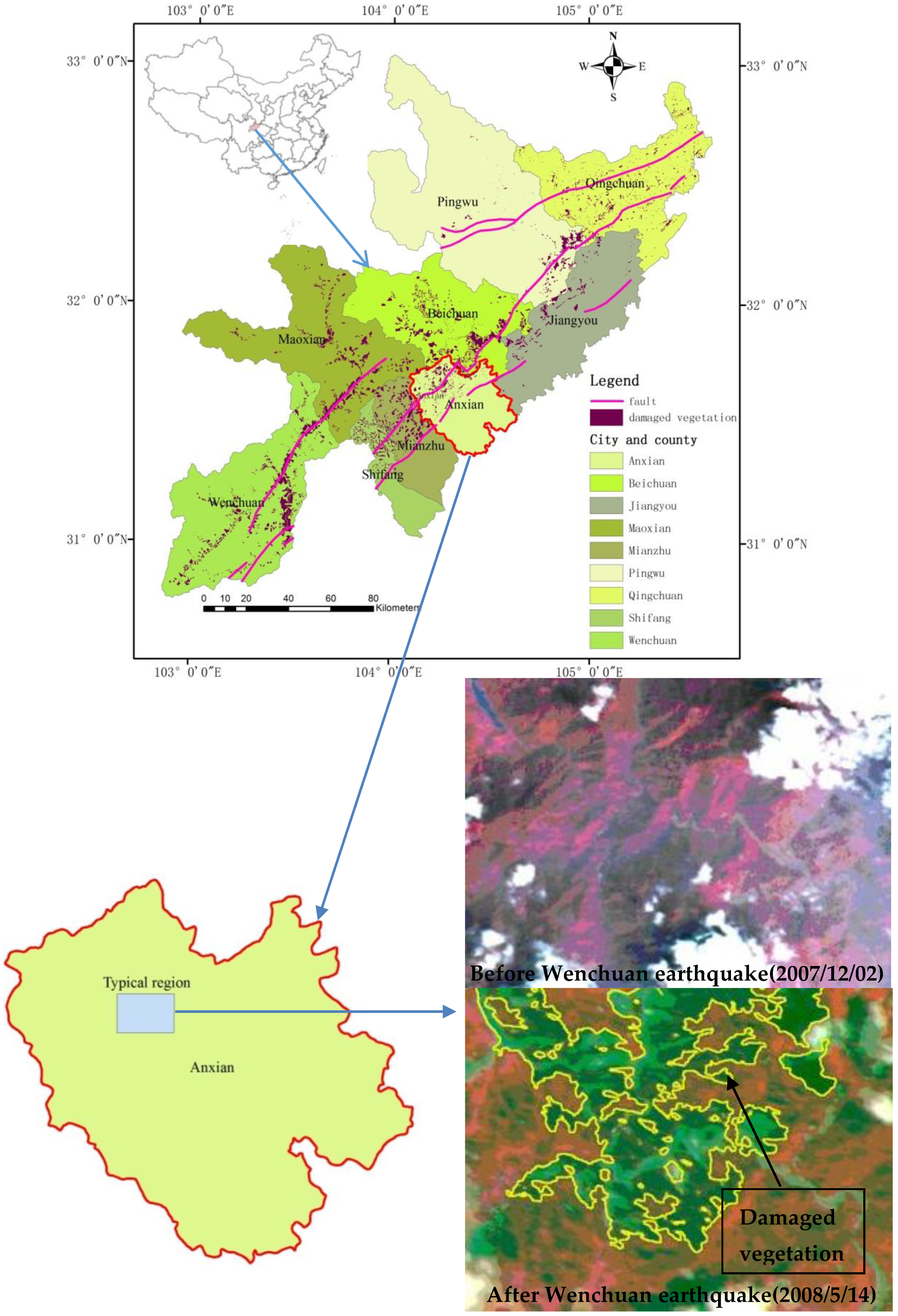
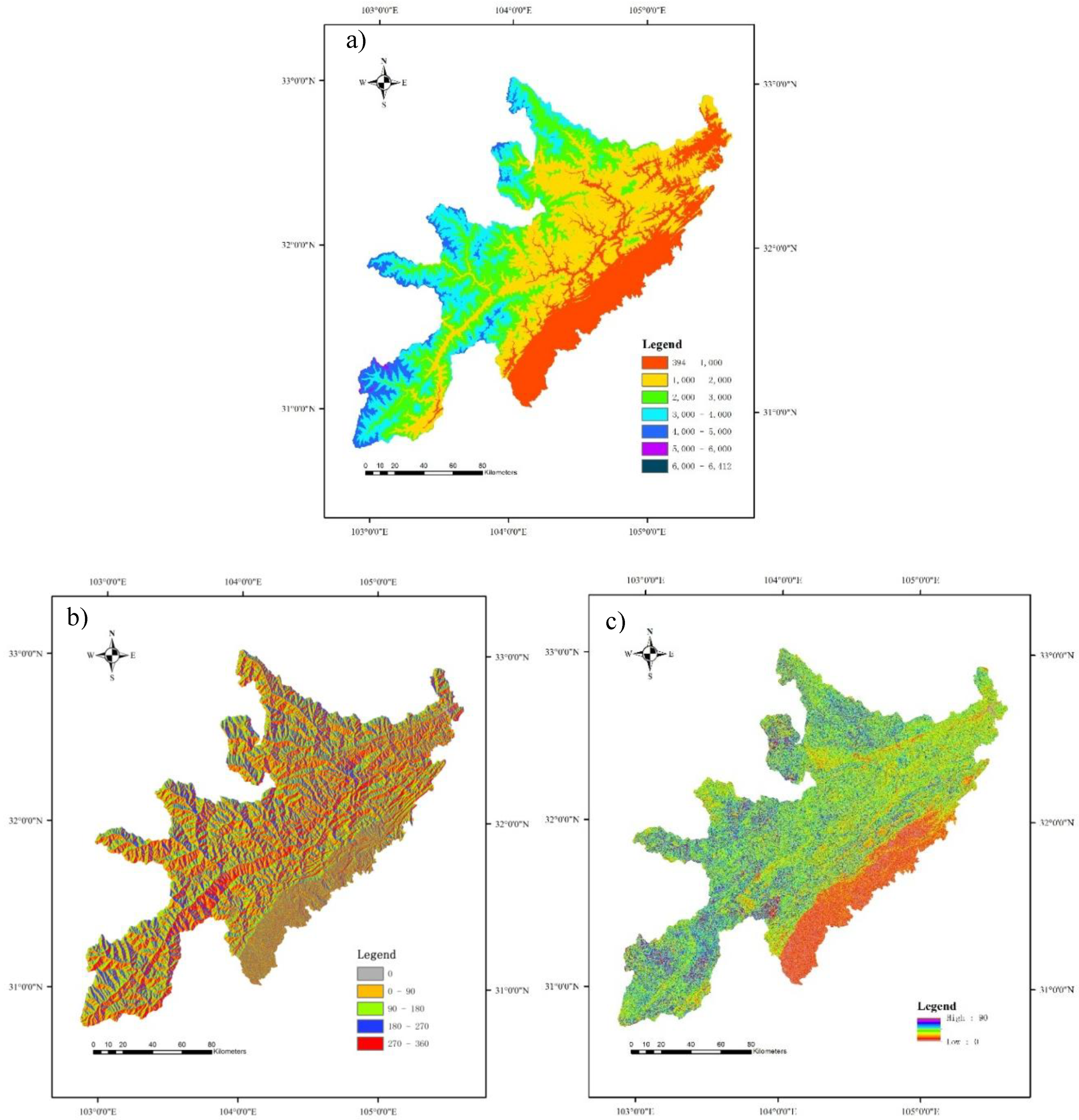
Nine severely damaged cities and counties—including Jiangyou, Mianzhu, Shifang, Beichuan County, Anxian County, Maoxian County, Pingwu County, Qingchuan County, and Wenchuan County—were chosen as our study area, where we collected data on topographic factors (including slope angles, orientations, distance to river, and elevation), seismic factors (including seismic intensity and distance to fault), human accessibility (including distances to road and residential area), and damaged vegetation. To thoroughly understand the relationship between the damaged vegetation and influencing factors in the Wenchuan earthquake-affected area, we used a spatial autocorrelation analysis to reveal the regional distribution, scale effect, and main influencing factors of damaged vegetation.

The main objectives of this study are (1) to characterize the spatial variability of damaged vegetation at different aggregation levels in the Wenchuan earthquake-affected area, (2) to identify the representative components of damaged vegetation, and (3) to clarify the main influencing factors on the spatial variability of damaged vegetation.

2. Materials and Methods

2.1. Study Area and Geological Setting

As seen in Figure 1, the nine cities and counties chosen for our study (N 30°45′~33°02′ and E 102°51′~105°38′) cover about 26,249 km² and are located at the eastern margin of the Tibetan Plateau in the most severely earthquake-affected areas of west Sichuan Province, China. They are characterized by semiarid hot and subtropical humid monsoon climates, with average annual precipitations of about 506 mm and 1503 mm, respectively. The mean annual temperatures are 13.8 and 15.0 ℃ respectively, and the mean annual evapotranspirations are 1392 mm and 1156 mm. From north to east, the elevation gradually decreases from 5230 to 462 m above sea level (a.s.l.), with a slope from 0° to 76°. The dominant soil types include brown soil, valley brown soil, and yellow soil.

The Wenchuan earthquake’s energy source was the famous active thrust Longmenshan fault, located at the conjunction of the Sichuan Basin western margin and the eastern edge of the Tibetan Plateau [24,25]. The Longmenshan fault initially formed in the Mesozoic and further developed throughout the Cenozoic from the collision of the Indian Plate onto the Eurasian Plate, resulting in the rapid uplift and tectonic deformation of the Longmenshan Mountain range [26]. The Longmenshan fault includes three regions: the Back fault, the Central fault, and the Front fault. As reverse faults, the Back and the Front faults consist of a series of reverse imbricate faults with a NE 250–450 orientation. They extend from Wenchuan County to Maoxian County and from Pengxian County to Guanxian County, respectively. Unlike the Back and the Front fault, the Central fault is a thrust fault with a NE 350–450 orientation, extending from the town of Yingxiu to Beichuan County. The Central fault and the Front fault both extend for 200 km and show dextral strike-slip movements along the eastern margin of the Tibetan Plateau, with higher slip rates (1–10 mm·yr⁻¹) than throw rates (<1 mm·yr⁻¹) since the Epipleistocene [25].

2.2. Data Collection

To investigate the spatial variation of damaged vegetation in the Wenchuan earthquake-affected area, information on the vegetation damage (

Table 1. The areas of different damaged vegetation types in nine worst-hit cities and counties (km²): Among all the vegetation types, we defined economic forests as the plantation that produces fresh or dry fruits, edible oils, beverages, spices, industrial raw materials, and medicinal materials.

Vegetation Type	Evergreen Broadleaf Forests	Deciduous Broadleaf Forests	Mixed Evergreen and Deciduous Broadleaf Forests	Mixed Broadleaf and Coniferous Forests	Deciduous Coniferous Forests	Evergreen Coniferous Forests	Economic Forests	Bamboo Forests	Shrubs	Meadows	Total
Area	69.74	122.64	120.15	42.24	10.50	184.99	268.12	5.71	338.60	86.79	1249.47
Patches	870	2245	2285	627	195	2669	4571	108	3165	691	17,426

) was extracted from an overlay analysis between the geo-hazard interpretations of remote sensing images from the China-Brazil Earth Resources Satellite (CBERS-02B) (Figure 1) and pre-earthquake vegetation distribution supplied by the Sichuan Forest Inventory and Planning Institution (SFIPI) [27]. The CBERS-02B images have a swath of 113 km and 5 wave bands, as seen in

Table 2. The 5 wavebands of a CBERS-02B CCD image.

Band No.	Spectral Range/nm
1	0.45–0.52
2	0.52–0.59
3	0.63–0.69
4	0.77–0.89
5	0.51–0.73

. To avoid the negative effects of cloud and haze on remote sensing images, 49 CBERS-02B CCD images containing 5 spectral bands (including red, green, blue, NIR1, and NIR2) with a pixel resolution of 19.5 m were acquired from May 14 to 28, 2008, excluding May 21 and 27 (

Table 3. The CBERS-02B CCD images used for the interpretation of geo-hazards distribution.

Date	Image Scene (Path/Row)	Number	Data Quality
2008.05.14	12/63, 12/64, 12/65	3	Some cloud covered
2008.05.15	11/62	1	Cloud and haze free
2008.05.16	11/63, 11/64, 11/65, 11/66, 11/67	5	Some cloud covered
2008.05.17	12/63, 12/64, 12/65, 12/66, 12/67	5	Some cloud covered
2008.05.18	11/63, 11/64, 11/65, 11/66, 11/67	5	Some cloud covered
2008.05.19	11/64, 11/65, 12/63, 12/66, 12/67	5	Some cloud covered
2008.05.20	12/63, 12/64, 12/65, 12/66	4	Some cloud covered
2008.05.22	11/63, 11/64, 11/65, 11/66, 11/67	5	Some cloud covered
2008.05.23	12/63, 12/64, 12/65, 12/66	4	Cloud and haze free
2008.05.24	10/63, 10/64, 10/65	3	Cloud and haze free
2008.05.25	11/64	1	Cloud and haze free
2008.05.26	11/63, 11/66, 11/67	3	Some cloud covered
2008.05.28	11/63, 11/64, 11/65, 11/66, 11/67	5	Some cloud covered

). This was the period during which the Chinese government reset the orbit parameter of CBERS-02B to monitor the geo-hazards daily following the Wenchuan earthquake. Due to spatial incompatibility between band-5 and the other bands in the CBERS-02B CCD images, we used the methods described by Li et al. [28] to re-project band-5 and then generated composite images using the re-projected band-5 and the other four bands. We applied the geometric correction using a second-order polynomial model with 24 ground control points (GCP) to ensure accuracy, based on primary scale Chinese national topographic maps (1:50,000). The spatial inconsistency errors were bounded within 1 pixel in this study. Subsequently, we interpreted the distribution of geo-hazards (including rock avalanches, landslides, debris flows, and landslide-dammed lakes) and used the GIS overlay analysis of pre-earthquake vegetation distribution, interpreted by SFIPI and the post-earthquake geo-hazards distribution, to determine the distribution of damaged vegetation, which was defined as a certain proportion of the pre-earthquake vegetation in a pixel, removed or destroyed by geo-hazards.

In this study, the digital elevation model (DEM) of the 25 m × 25 m cell size Sichuan Province study area (Figure 2), provided by the Institute of Mountain Hazards and Environment, was used to calculate and extract the topographic factors, including river systems, elevation, slope, and aspect (Figure 2), with the spatial analyst tools in ARC/INFO 9.2. The fundamental geographic information features of 1:250,000 for the Sichuan Province, including roads and residential areas, were chosen as proxies for human accessibility. The fault data were extracted from the map of horizontal peak ground acceleration (PGA) in the Wenchuan earthquake-affected area, created by Tang et al. [29]. In addition, the seismic intensity zone data were extracted from the Ms 8.0 Wenchuan earthquake seismic intensity map created by Xu et al. [30]. All data were combined with the damaged vegetation data using an overlay analysis. In this study, a set of 19 potential drivers of earthquake damage degree (

Table 4. The damaged vegetation types and potential drivers used in the statistical analysis in nine severely damaged cities and counties.

Variable	Code	Unit
Damaged vegetation types
Percentage of all damaged vegetation	A
Percentage of bamboo forests	B
Percentage of mixed broadleaf and coniferous forests	C
Percentage of deciduous broadleaf forests	D
Percentage of deciduous coniferous forests	E
Percentage of economic forests	F
Percentage of evergreen broadleaf forests	G
Percentage of evergreen coniferous forests	H
Percentage of meadows	I
Percentage of mixed evergreen and deciduous broadleaf forests	J
Percentage of shrubs	K
Drivers
Elevation	elevation	m a.s.l.
Percentage of slope class 1 (0–10°)	slope0_10
Percentage of slope class 2 (10–20°)	slope10_20
Percentage of slope class 3 (20–30°)	slope20_30
Percentage of slope class 4 (>30°)	slope30
Percentage of north slope (270–360°)	270_360
Percentage of west slope (180–270°)	180_270
Percentage of south slope (90–180°)	90_180
Percentage of east slope (0–90°)	0_90
Percentage of flat area (0°)	flat
Distance to nearest urban centre	county_dis	km
Distance to nearest road	road_dis	km
Distance to nearest river	river_dis	km
Distance to nearest fault	fault_dis	km
Percentage of VII seismic intensity zone	VII_area
Percentage of VIII seismic intensity zone	VIII_area
Percentage of IX seismic intensity zone	IX_area
Percentage of X seismic intensity zone	X_area
Percentage of XI seismic intensity zone	XI_area

) were selected for the damaged vegetation at four different aggregation levels. The highest resolution in the data set is 1 × 1 (625 × 625 m) grid cells. With the accumulative data of 2 × 2, 4 × 4, and 8 × 8 grid cells, a total of four aggregation levels were created to simulate different scales using the methods described in Overmars et al. [19].

2.3. Spatial Autocorrelation Analysis

Spatial autocorrelation is defined as the phenomenon of geographic proximity’s potential to determine the values of random variables over distances that are similar or dissimilar to randomly associated pairs of observations [31]. Researchers have used spatial autocorrelation to describe the dependency and covariance of variables within a spatial neighborhood [32,33,34].

2.3.1. Global Spatial Autocorrelation Statistics

Correlograms calculated with univariate (Moran’s I or Geary’s c) and multivariate data (Mantel correlogram) can be used to quantify the spatial dependency per distance class [35,36,37]. In this study, we used correlograms of the Moran’s I as described in Overmars et al. [19]. The formula is expressed as follows [31]:

Moran’s I for h ≠ i:

$$\mathrm{I}\left(\mathrm{d}\right)=\frac{\left(1/W\right){\sum }_{h=1}^n{\sum }_{i=1}^n{w}_{hi}(y_h-\overline{y})\left(y_i-\overline{y}\right)}{\left(\frac{1}{n}\right){\sum }_{i=1}^n{(y_i-\overline{y})}^2}$$

(1)

where y_h and y_i are the values of the observed variable at sites h and i, respectively; the values of w_hi are weight matrices; and W in a (n × n) weight matrix is the sum of the weights w_hi for a given distance class, i.e., the number of pairs used to calculate the coefficient.

Moran’s I can be calculated using a free software, Geoda [38], in which the value of Moran’s I generally ranges from −1 to 1. High positive Moran’s I values indicate a positive autocorrelation, which implies the clustering of similar values; low negative values, by contrast, represent a negative autocorrelation, which implies the clustering of dissimilar values. A value close to zero indicates no autocorrelation [39,40,41].

2.3.2. Local Spatial Autocorrelation Statistics

Global spatial autocorrelation may not pick up the aberrant local spatial pattern that causes some local patterns to be opposite to the global spatial trend [41]. To assess the influence of aberrant local spatial patterns on the magnitude of the global statistic, Anselin [42] outlined a class of local indicators of spatial association (LISA) (1) to assess the extent of significant local spatial clustering around an individual location, (2) to indicate the local pockets of spatial non-stationarity, and (3) to identify outliers or spatial regimes. The formula expressed in the form of a LISA is as follows [42]:

$$I_i=\frac{\left(y_i-\overline{y}\right)}{{\sum }_{i=1}^n{(y_i-\overline{y})}^2}{\displaystyle \sum }_{j=1}^n{w}_{ij}\left(y_i-\overline{y}\right)$$

(2)

Local Moran’s I can also be calculated by “GeoDa” with some visualization results—the significance map of Moran’s I and spatial clustering [38].

2.3.3. Spatial Autoregressive Models

To avoid the effects of the biased estimation of error variance, t-test significance levels, and the overestimation of R² caused by conventional statistical methods when dealing with spatial autocorrelation, a commonly used spatial autoregressive model is Equation (3) created by Anselin [43]. From Equation (3), we can derive several specific models by imposing restrictions [19,44]. Setting W₂ × 0 produces a spatial lag model (SLM) or mixed regressive-spatial autoregressive model (Equation (4)) and expresses how the magnitude of a decision variable for a geographical grid depends on the magnitudes of the decision variables set by other grids [44,45]. This model can explain the additional variation y over the spatial sample via additional explanatory variables in the matrix X [43]. Setting W₁ = 0 produces a spatial error model (SEM) (Equation (5)) and describes the spatial autocorrelation in the disturbances [44].

$$y=\rho W_{1}y+X\beta +u\hspace{1em}\hspace{1em}u=W_{2}u+\epsilon \hspace{1em}\hspace{1em}\epsilon ~N\left(0,{\sigma }^2{I}_n\right)$$

(3)

$$y=\rho W_{1}y+X\beta +\epsilon \hspace{1em}\hspace{1em}\epsilon ~N\left(0,{\sigma }^2{I}_n\right)$$

(4)

$$y=X\beta +u\hspace{1em}\hspace{1em}u=W_{2}u+\epsilon \hspace{1em}\hspace{1em}\epsilon ~N\left(0,{\sigma }^2{I}_n\right)$$

(5)

In Equations (3)–(5), y is an n × 1 vector of cross-sectional dependent variables and X contains an n × k matrix of explanatory variables with an associated k × 1 regression coefficient vector β. W₁ and W₂ are n × n spatial weight matrices describing the interconnections between different locations, ρ is the coefficient of the spatially lagged dependent variable, λ is the coefficient of the spatially correlated errors, and ε is a vector or random error term [19,46].

In this study, two spatial autoregressive models (Equations (4) and (5)) are used. The maximum likelihood estimation is used to estimate the parameters in GeoDa, since an ordinary least squares estimation for spatial autoregressive models is biased [38]. We use the pseudo R² (defined as the ratio of variance of the predicted values over the variance of the observed values for the dependent variable) and the value of the maximized log likelihood (LIK) to assess the fit in the spatial autoregressive models and all other models [19,44]. In addition, we select the ρ value and its significance as the percentage of the prediction that is obtained using the spatial part and the significance of spatial autocorrelation [19].

2.4. Data Analysis

GeoDa was used to calculate the Moran’s I statistic. The weight matrices were established based on distance [47] and were equal within a lag. The lag sizes chosen were 625 m, 1250 m, 2500 m, and 5000 m, respectively at the 1 × 1, 2 × 2, 4 × 4, and 8 × 8 aggregation levels. Correlograms were calculated and compared for all combinations of the four aggregation levels, driving factors, and ten vegetation types. Within a same lag, we used correlograms pairs between the Moran’s I of the percentage of all damaged vegetation and ten vegetation types to create regression models to determine their relationships.

To calculate SLM and SEM, GeoDa was used as well. We used the independent variables selected method of de Koning et al. [48] to remove insignificant variables one by one until a model with only significant variables remained.

3. Results

3.1. Spatial Autocorrelation Testing

3.1.1. Relationships between Correlograms of All Destructed Vegetation and Ten Vegetation Types at the Four Cell Levels

As seen in Figure 3, the correlograms of the Moran’s I (distances as 625 m, 1250 m, 2500 m, and 5000 m of a lag respectively) of the percentage of all the damaged vegetation and ten vegetation types are presented in 1 × 1, 2 × 2, 4 × 4, and 8 × 8 cells. The correlograms showed large differences in Moran’s I between vegetation types. All the damaged vegetation and ten vegetation types, represented in Figure 3, showed a significantly positive spatial autocorrelation (P < 0.001), which decreased gradually and still had a significant autocorrelation with distance at all four aggregation levels. All damaged vegetation, economic forests, evergreen coniferous forests, meadows, and shrubs had a comparatively high Moran’s I across the lag distances at all four aggregation levels. Moran’s I of ten vegetation types were significantly related to that of all the destructed vegetation across the lag distances at all four aggregation levels (

Table 5. The regression models between the Moran’s I of ten vegetation types and those of all the destructed vegetation across the lag distance of 625 m, 1250 m, 2500 m, and 5000 m comparatively at four corresponding aggregation levels. The vegetation type abbreviations are defined in Table 4.

Vegetation Types	Grid Cells
	625 m			1250 m			2500 m			5000 m
	Regression Model	R2	P	Regression Model	R2	P	Regression Model	R2	P	Linear Model	R2	P
B	y = 0.0038e7.1518x	0.9856	<0.001	y = 0.0038e5.8931x	0.9889	<0.001	y = 0.2607x1.3364	0.9863	<0.001	y = 0.7096x − 0.0223	0.9928	<0.001
C	y = 0.7278x1.7546	0.9988	<0.001	y = 0.7235x1.6897	0.9990	<0.001	y = 0.0183e5.2466x	0.9911	<0.001	y = 0.7119x1.3877	0.9798	<0.001
D	y = 0.7577x1.5143	0.9912	<0.001	y = 0.6330x1.2145	0.9888	<0.001	y = 0.7096x − 0.0223	0.9958	<0.001	y = 0.7636x − 0.0202	0.9964	<0.001
E	y = 0.0160e4.9371x	0.9861	<0.001	y = 0.6781x1.6046	0.9930	<0.001	y = 1.0191x1.6421	0.9926	<0.001	y = 0.0142e6.0289x	0.9909	<0.001
F	y = 0.9241x1.3444	0.9999	<0.001	y = 0.8630x1.2584	0.9988	<0.001	y = 0.8497x − 0.0413	0.9943	<0.001	y = 0.7695x − 0.0224	0.9941	<0.001
G	y = 0.8571x1.7323	0.9978	<0.001	y = 0.7468x1.6324	0.9996	<0.001	y = 0.0174e5.3293x	0.9791	<0.001	y = 0.3571x0.9674	0.9819	<0.001
H	y = 0.7944x1.3188	0.9938	<0.001	y = 0.6699x1.1353	0.9920	<0.001	y = 0.6377x + 0.0033	0.9946	<0.001	y = 0.7324x + 0.0241	0.9889	<0.001
I	y = 0.9775x − 0.0922	0.9982	<0.001	y = 1.1385x1.5587	0.9996	<0.001	y = 0.7920x1.4135	0.9834	<0.001	y = 0.5267x1.1235	0.9817	<0.001
J	y = 0.0400e4.0595x	0.9911	<0.001	y = 0.6667x1.1313	0.9966	<0.001	y = 0.7435x − 0.0207	0.9986	<0.001	y = 0.8440x + 0.0360	0.9982	<0.001
K	y = 0.9305x − 0.0324	0.9995	<0.001	y = 0.9545x − 0.0321	0.9989	<0.001	y = 0.9729x − 0.0339	0.9958	<0.001	y = 0.8864x − 0.0100	0.9945	<0.001

), indicating that the components of all the destructed vegetation could represent the characteristics of its spatial autocorrelation. However, unlike the other vegetation types having exponential function or power function relationships with all destructed vegetation, shrubs had linear function relationships with all the destructed vegetation at all four aggregation levels (Table 5).

3.1.2. Correlograms of Potential Driving Factors at the 1 × 1 Cell Level

Except for four slope aspects (the east, south, west, and north slopes) with comparatively lower Moran’s I (Moran’s I < 0.200), all potential driving factors showed a significantly positive spatial autocorrelation (P < 0.001) with a comparatively high Moran’s I (ranging from 0.338 to 0.793) at the 1 × 1 cell level, which also decreased gradually with distance (Figure 4a–d).

3.1.3. LISA Map of All Damaged Vegetation at the 1 × 1 Cell Level

As seen in Figure 5, the cluster and significance maps of LISA for all damaged vegetation at the 1 × 1 aggregation level indicate that the high-high zone occupied 4146 out of 4854 grid cells with <0.05 significance levels. This means that a clustering of similar high coverage of damaged vegetation occurred in the Wenchuan earthquake-affected area, causing a highly fragmented wildlife habitat at range-wide scales and the loss of a global biodiversity hotspot [17,49].

3.1.4. Spatial Autocorrelation in Residuals

In this study, we used the residuals of the standard linear regression models in the first lag constructed by Overmars et al. [19] to determine the scale threshold of the aggregation levels. The residuals’ spatial autocorrelation in the first lag of all aggregation levels were significant in all the destructed vegetation and ten vegetation types with Moran’s I > 0.130 except for the bamboo forest vegetation type at the aggregation level 8 × 8 (

Table 6. Moran’s I of the residuals in the first lag at different aggregation levels.

Vegetation Type	Aggregation Level
	1 × 1	2 × 2	4 × 4	8 × 8
All damaged vegetation	0.319	0.332	0.335	0.273
Bamboo forests	0.284	0.168	0.133	0.066
Mixed broadleaf and coniferous forests	0.336	0.280	0.323	0.289
Deciduous broadleaf forests	0.376	0.329	0.329	0.265
Deciduous coniferous forests	0.333	0.270	0.329	0.310
Economic forests	0.365	0.338	0.354	0.257
Evergreen broadleaf forests	0.399	0.293	0.274	0.170
Evergreen coniferous forests	0.403	0.318	0.242	0.268
Meadows	0.485	0.450	0.352	0.263
Mixed evergreen and deciduous broadleaf forests	0.424	0.347	0.340	0.307
Shrubs	0.425	0.392	0.405	0.301

The numbers in bold font are not significant (P > 0.001).

). Moreover, the residuals’ spatial autocorrelation weakened at aggregation levels 4 × 4 and 8 × 8, suggesting that the aggregation level 8 × 8 may be a scale threshold for spatial autocorrelation.

3.2. Results of Spatial Autoregressive Models

We used the standard linear model based on ordinary least squares, spatial lag model (SLM), and spatial error model (SEM) as spatial autoregressive models to illustrate their differences in all damaged vegetation at aggregation level 1 × 1 (

Table 7. The model parameters of three different models for all damaged vegetation at aggregation level 1 × 1.

Variable	Coefficient	S.D.	t-Statistic	Probability
(1) Linear model
Constant	0.0041	0.0019	2.1762	0.0296
Distance to nearest river (km)	−0.0076	0.0002	−37.5753	0
Distance to nearest fault (km)	−0.0017	0.0001	−12.2201	0
Distance to nearest road (km)	−0.0014	0.0002	−7.2000	0
Distance to nearest urban centre (km)	0.0032	0.0003	11.8087	0
Elevation (m a.s.l.)	2.14 × 10−5	1.75 × 10−6	12.2063	0
Percentage of slope class 2 (10–20°)	0.1960	0.0114	17.1561	0
Percentage of slope class 3 (20–30°)	0.1566	0.0088	17.7884	0
Percentage of slope class 4 (>30°)	0.1915	0.0082	23.3667	0
Percentage of south slope (180–270°)	−0.0155	0.0076	−2.0262	0.0428
Percentage of VIII seismic intensity zone	0.1022	0.0072	14.2505	0
Percentage of IX seismic intensity zone	0.0928	0.0074	12.4649	0
Percentage of X seismic intensity zone	0.1497	0.0076	19.6639	0
Percentage of XI seismic intensity zone	0.1987	0.0080	24.9411	0
R2	0.5053
Log likelihood (LIK)	54592.9
Variable	Coefficient	S.D.	Z-value	Probability
(2) Spatial lag model
ρ	0.5566	0.0032	172.0463	0
Constant	−0.0037	0.0016	−2.3945	0.0166
Distance to nearest river (km)	−0.0034	0.0002	−20.4096	0
Distance to nearest fault (km)	−0.0006	0.0001	−5.5366	0
Distance to nearest road (km)	−0.0010	0.0002	−6.3301	0
Distance to nearest urban centre (km)	0.0010	0.0002	4.3178	0
Elevation (m a.s.l.)	1.24 × 10−5	1.44 × 10−6	8.6397	0
Percentage of slope class 2 (10–20°)	0.1097	0.0094	11.7252	0
Percentage of slope class 3 (20–30°)	0.0965	0.0072	13.3727	0
Percentage of slope class 4 (>30°)	0.1080	0.0067	16.0661	0
Percentage of south slope (180–270°)	−0.0048	0.0062	−0.7753	0.4382
Percentage of VIII seismic intensity zone	0.0546	0.0059	9.2862	0
Percentage of IX seismic intensity zone	0.0523	0.0061	8.5668	0
Percentage of X seismic intensity zone	0.0755	0.0063	12.0679	0
Percentage of XI seismic intensity zone	0.0942	0.0066	14.3581	0
R2	0.6685
Log likelihood (LIK)	64938.3
(3) Spatial error model
ρ	0.5923	0.0036	163.659	0
Constant	0.0149	0.0009	16.5203	0
Distance to nearest river(km)	−0.0049	0.0003	−19.5888	0
Distance to nearest fault(km)	−0.0007	0.0002	−3.8453	0.0001
Distance to nearest road(km)	−0.0026	0.0003	−10.4537	0
Distance to nearest urban centre(km)	−3.43 × 10−5	0.0004	−0.0942	0.9250
Elevation (m a.s.l.)	1.68 × 10−5	2.15 × 10−6	7.8162	0
Percentage of slope class 2 (10–20°)	0.1028	0.0106	9.6784	0
Percentage of slope class 3 (20–30°)	0.1052	0.0085	12.4366	0
Percentage of slope class 4 (>30°)	0.1174	0.0080	14.6208	0
Percentage of VIII seismic intensity zone	0.0908	0.0075	12.1203	0
Percentage of IX seismic intensity zone	0.0935	0.0076	12.2432	0
Percentage of X seismic intensity zone	0.1377	0.0080	17.3240	0
Percentage of XI seismic intensity zone	0.1769	0.0086	20.5106	0
R2	0.6416
Log likelihood (LIK)	61732.3

).

The standard linear model contains thirteen significant variables (P > 0.05) selected using a stepwise regression from a set of 19 potential drivers with parameters including the measure of fit (R²), coefficient estimate, standard error, t-test value, associated probability, and log likelihood (LIK) (Table 7(1)). We used the LIK to compare the goodness-of-fit of three spatial models. From Table 7(2), we found that the spatial lag model had smaller estimated regression coefficients and standard errors, as well as a higher R², using the same variables in the standard linear model. The significance of the parameters decreased as well, and the variable “Percentage of south slope (180–270°)” was no longer significant (P < 0.05). Moreover, the spatial lag model has a higher LIK than the standard linear model, indicating a better goodness-of-fit.

Based on the results of the spatial lag model, we excluded the insignificant variable to construct the spatial error model. From Table 7(3), we found that the pseudo R² and the LIK of the spatial error model decreased from 0.6685 to 0.6416 and from 64,938.3 to 61,732.3 compared with the spatial lag model, indicating that excluding the insignificant variable only results in a slight reduction of the goodness-of-fit.

The spatial autocorrelation in the residuals of spatial lag and spatial error models weakened (Figure 6). Furthermore, the difference in their spatial autocorrelations was negligible. Compared to the spatial lag and spatial error models, the standard linear model had larger residuals with a positive spatial autocorrelation. For example, as seen in

Table 8. The grids and percentages of the residuals of the standard linear model switched to the spatial error model at aggregation level 1 × 1.

	Grids of Positive Residuals of the Standard Linear Model		Grids of Negative Residuals of the Standard Linear Model
Switched to the spatial error model	Negative/Less positive	More positive	Positive/Less negative	More negative
	264/2110 (2.50%/19.94%)	1854 (17.52%)	741/4439 (7.00%/41.95%)	1173 (11.09%)
Coverage of all damaged vegetation > 60%	1079 (10.20%)	465 (4.39%)	-	-
Coverage of all damaged vegetation < 20%	32 (0.30%)	69 (0.65%)	4332 (40.94%)	808 (7.64%)

, more grids with a comparatively higher/lower original value of the residuals of the standard linear model are switched from positive/negative to negative/positive or less positive/negative. Therefore, the residuals of the spatial error model are considerably lower.

We list some models’ outputs for all the destructed vegetation and ten vegetation types (

Table 9. A summary of the spatial error model for all vegetation types at four aggregation levels.

Vegetation Type	Aggregation Level	ρ	Number of Variables (Number of Variables in the Standard Linear Model)
All damaged vegetation	1 × 1	0.5923	12 (13)
Bamboo forests	1 × 1	0.4611	7 (7)
Mixed broadleaf and coniferous forests	1 × 1	0.5196	6 (8)
Deciduous broadleaf forests	1 × 1	0.5581	11 (11)
Deciduous coniferous forests	1 × 1	0.5322	7 (8)
Economic forests	1 × 1	0.5779	10 (10)
Evergreen broadleaf forests	1 × 1	0.6012	8 (10)
Evergreen coniferous forests	1 × 1	0.6118	7 (9)
Meadows	1 × 1	0.6629	11 (11)
Mixed evergreen and deciduous broadleaf forests	1 × 1	0.6115	11 (11)
Shrubs	1 × 1	0.6545	9 (12)
All damaged vegetation	2 × 2	0.6077	11 (12)
Bamboo forests	2 × 2	0.3080	7 (7)
Mixed broadleaf and coniferous forests	2 × 2	0.4397	6 (6)
Deciduous broadleaf forests	2 × 2	0.5287	11 (11)
Deciduous coniferous forests	2 × 2	0.4317	7 (8)
Economic forests	2 × 2	0.5511	10 (10)
Evergreen broadleaf forests	2 × 2	0.4752	9 (10)
Evergreen coniferous forests	2 × 2	0.5428	7 (8)
Meadows	2 × 2	0.6579	9 (10)
Mixed evergreen and deciduous broadleaf forests	2 × 2	0.5497	11 (11)
Shrubs	2 × 2	0.6457	10 (12)
All damaged vegetation	4 × 4	0.6153	9 (11)
Bamboo forests	4 × 4	0.2422	5 (5)
Mixed broadleaf and coniferous forests	4 × 4	0.5062	4 (6)
Deciduous broadleaf forests	4 × 4	0.5233	9 (9)
Deciduous coniferous forests	4 × 4	0.4699	2 (5)
Economic forests	4 × 4	0.5750	10 (10)
Evergreen broadleaf forests	4 × 4	0.4180	5 (6)
Evergreen coniferous forests	4 × 4	0.4301	5 (6)
Meadows	4 × 4	0.5295	6 (7)
Mixed evergreen and deciduous broadleaf forests	4 × 4	0.5408	10 (10)
Shrubs	4 × 4	0.6505	7 (9)
All damaged vegetation	8 × 8	0.5261	7 (7)
Bamboo forests	8 × 8	0.0943 *	5 (5)
Mixed broadleaf and coniferous forests	8 × 8	0.5005	4 (4)
Deciduous broadleaf forests	8 × 8	0.4285	9 (9)
Deciduous coniferous forests	8 × 8	0.5050	2 (5)
Economic forests	8 × 8	0.4681	9 (9)
Evergreen broadleaf forests	8 × 8	0.2883	2 (5)
Evergreen coniferous forests	8 × 8	0.5270	6 (6)
Meadows	8 × 8	0.4574	6 (7)
Mixed evergreen and deciduous broadleaf forests	8 × 8	0.5462	6 (10)
Shrubs	8 × 8	0.5303	6 (8)

* Not significant (P < 0.05).

). Based on the guidance of Overmars et al. [19], which states that the significance of ρ is a criterion of whether to apply the spatial error model, 43 out of our 44 models qualified for applying the spatial model. All ρ values at all four aggregation levels were significant except for bamboo forests at the 8 × 8 aggregation level, indicating that the vegetation types may have a patch size smaller than the cell size over the 8 × 8 aggregation level. Therefore, the aggregation level 8 × 8 may be a scale threshold for spatial autocorrelation in damaged vegetation of the Wenchuan earthquake-affected area.

In this study, the spatial error model accounts for 46.11–66.29% of the prediction at the 1 × 1 aggregation level. There are additional environmental factors, including other independent variables, affecting the vegetation destruction in the Wenchuan earthquake-affected area.

4. Discussion

It has been proven that spatial autocorrelation is present in most data and that traditional methods such as linear regression are positively misleading [50,51,52]. Spatial autocorrelation allows us to understand spatial patterns and can help avoid pitfalls in multiple regression analyses at macro or small scales. However, it cannot explain the variation in research objectives because the adjacent cells do not represent the response of research objectives to variations in the driving environmental factors [51,53]. Hence, spatially structured environmental factors that are independent of the variable of interest can cause objectives to be spatially structured [54]. In addition, to our knowledge, there is almost no information in the literature about whether the components of research objectives can be a valid indicator that reflects the characteristics of research objectives’ spatial autocorrelation. To elucidate the main factors influencing the degree of vegetation damage and to find out the key vegetation type to reflect the spatial autocorrelation of destructed vegetation is the basis of regionalized countermeasures in vegetation protection and conservation in earthquake-affected areas. Thus, statistical models should be applied to explain the correlation between vegetation destruction, its components, and the driving environmental factors using methods such as spatial generalized least-squares (GLS) or autoregressive models [31].

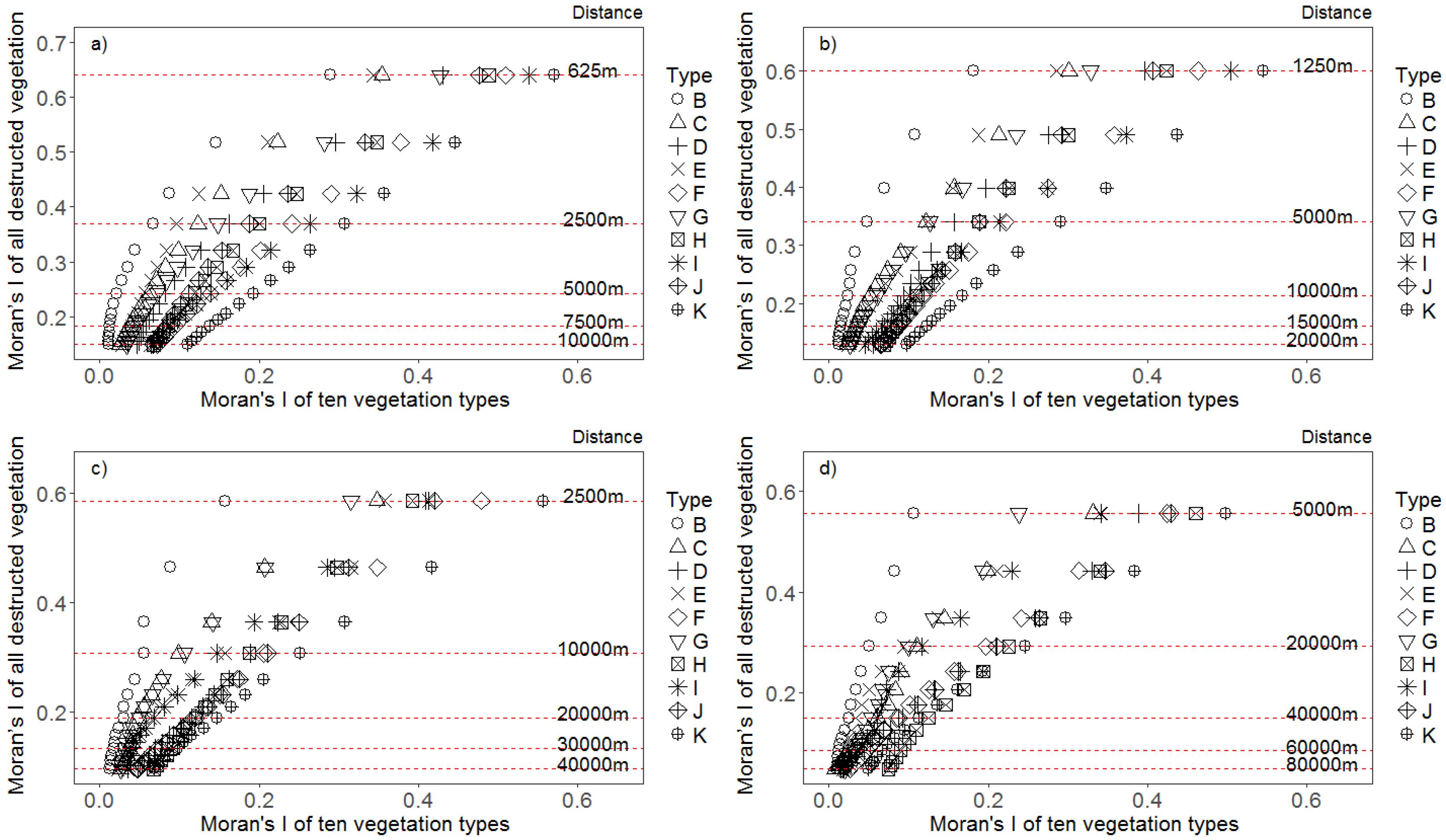
Vegetation destruction caused by the Wenchuan earthquake reached 1249.47 km² in our study area, accounting for 4.76% of the area of the nine worst-hit cities and counties [1]. There was a significantly positive spatial autocorrelation in all the damaged vegetation and its components. However, the Moran’s I values of the surface percentage within cells of the 11 vegetation types are clearly different at all four aggregation levels. This means that vegetation types have different patterns and different spatial characteristics within the different categories of all damaged vegetation. In fact, any categorization made with our prior knowledge can cause the differences (y_h − y_i) for any distance d, independent of the location where the differences are calculated [31]. Therefore, each vegetation category reflecting the spatial distribution of all the damaged vegetation or not may show similar or different spatial patterns to all the damaged vegetation. To assess the importance of each vegetation category in the whole and to determine the main damaged vegetation type contributing substantially towards the design of restoration programs by demonstrating the importance of accounting for species selection and local conditions, we set up regression models between the Moran’s I of ten vegetation types and those of all the destructed vegetation across the corresponding lag distances at all four aggregation levels. We found that the Moran’s I of ten vegetation types had significant relationships (including exponential function, power function, and linear function) with that of all the destructed vegetation. However, unlike the other vegetation types, only shrubs had significantly positive linear relationships with all the destructed vegetation at all four aggregation levels, indicating that the Moran’s I of shrubs decreases with distance following the same rule as all destructed vegetation. In other words, shrubs can represent the characteristics of the spatial structure of all damaged vegetation to a certain extent and may play an important proxy role in designing vegetation restoration plans for the Wenchuan earthquake-affected area. Similar effects to shrub vegetation type were reported in previous studies, showing that it is the main vegetation type distributed between 1800 and 3400 m a.s.l. for headwater and animal habitat conservation efforts in our study area [1,55]. The other vegetation types show a significant exponential function or power function with all destructed vegetation, indicating that their spatial autocorrelation attenuate more quickly than all the destructed vegetation with increasing distance. This means that the other vegetation types cannot reflect the spatial autocorrelation of all the destructed vegetation except shrubs when the patch size is smaller than the cell size over a certain distance. This result is consistent with other studies demonstrating significant impacts of patch size on spatial structure [19].

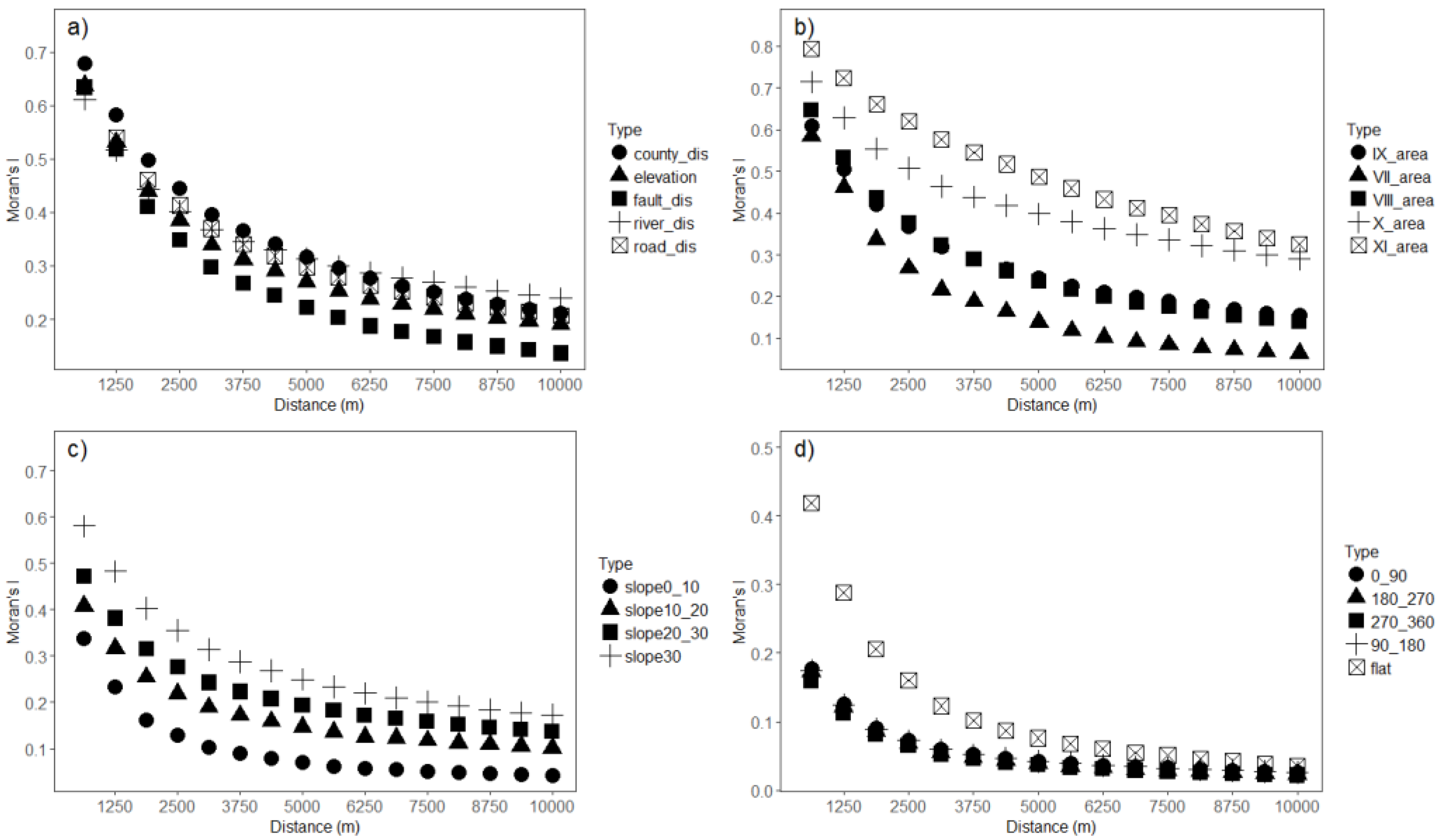
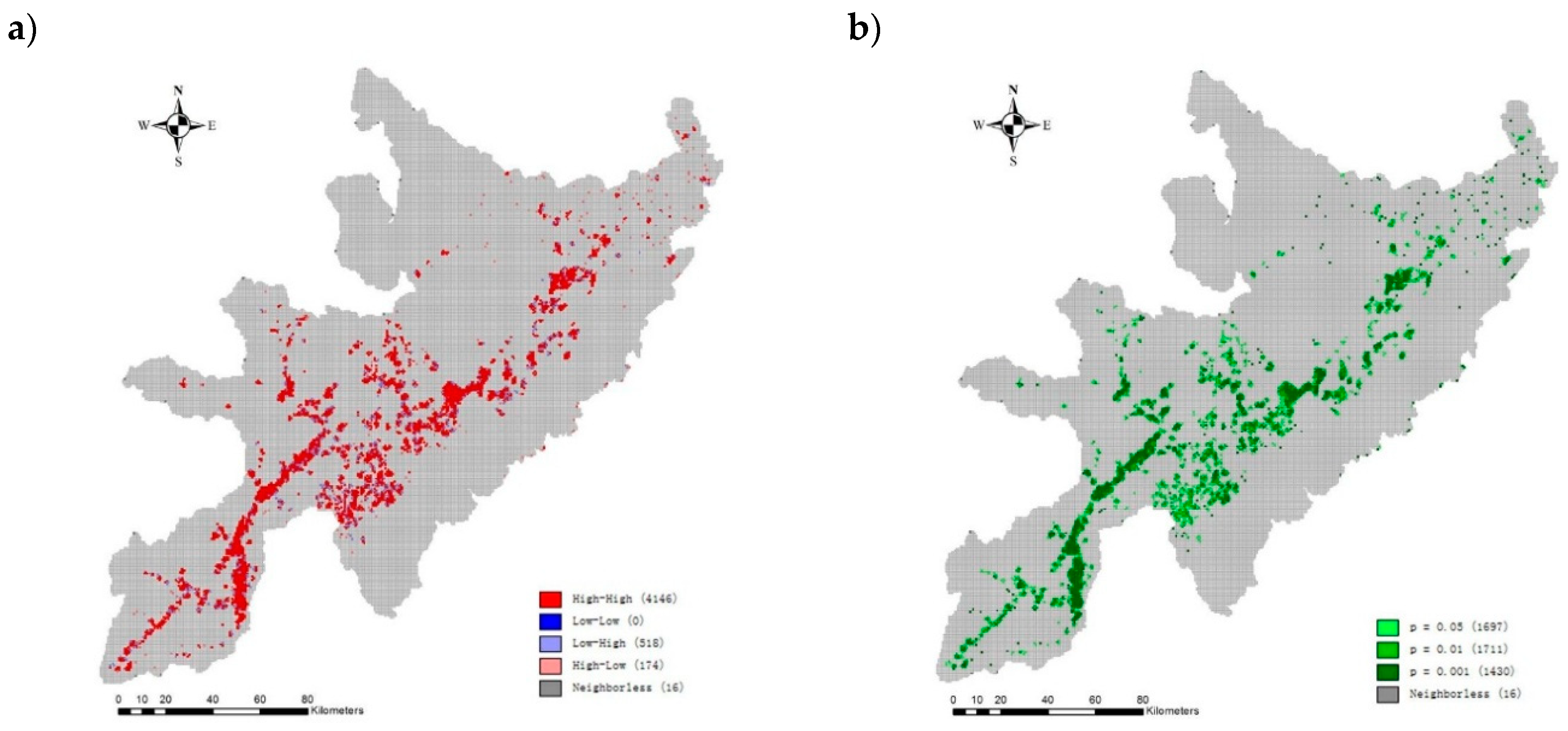
The spatial structures of 19 potential driving factors also showed a significantly positive spatial autocorrelation (Figure 4). This means that the characteristics of damaged vegetation may be explained by driving forces, depending on the response of land use and cover to driving factors [19]. Cluster and significance maps of LISA can enable us to assess the interactions between sites in close proximity to each other by comparing their values to their neighbors and identifying the local spatial structure and instability [41]. In this study, LISA maps delineated damaged vegetation zones in accordance with the types of spatial autocorrelation. Therefore, spatial autoregressive models should be used to detect the relationships between damaged vegetation and driving factors.

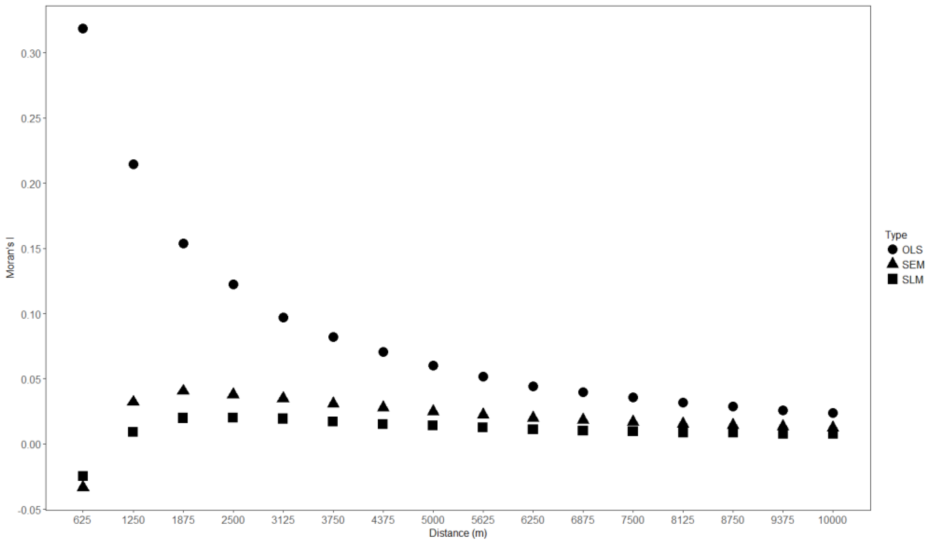
In all the destructed vegetation and ten vegetation types at all aggregation levels (Figure 3 and Table 6), the residuals’ spatial autocorrelation of the standard linear regression is less than that of the original data, indicating that the selected driving factors used in the linear regression model are partly responsible for vegetation destruction or that damaged vegetation is a response to the spatially autocorrelated selected driving factors. However, the residuals’ spatial autocorrelation is still significant, indicating that the standard linear model is not enough to explain all spatial patterns.

Spatial autoregressive models can be used to reduce or remove the spatial patterns of standard linear model residuals [53]. Though the pseudo R² in spatial models cannot be used in comparison with the traditional R² in the standard linear model for a measure of fit, the value of the maximized log likelihood (LIK) can be used to determine the goodness-of-fit of different models [44]. In this study, spatial autoregressive models have a higher LIK than the standard linear model, indicating a better goodness-of-fit (Table 7). Comparing the residuals of the spatial lag model and spatial error model with the standard linear model (Figure 6), we found that they are considerably lower when using the spatial models. Though it may seem controversial or unsatisfactory that the prediction of a variable should use neighboring values, unlike the standard linear model which only focuses on the dominant effects caused by responses to driving forces, spatial models can deal with spatial interactions that cannot be included in the standard linear model [18,31]. Moreover, compared to the spatial error model, low original values result in large negative residuals and high original values result in large positive residuals in the standard linear model (Table 8). However, our study showed that the residuals of the spatial lag model and spatial error model still had significant spatial autocorrelations. This may be due to the absence of some important environmental variables which are not available at a required spatial resolution [53,56]. Therefore, more comprehensive spatial modeling techniques considering the multicollinearity of environmental variables may be a strategy to improve the model fit [53,57].

There is a scale threshold in aggregation levels that causes lower and even insignificant spatial autocorrelation at the 8 × 8 aggregation level than aggregation levels 4 × 4 (Table 6). Although the omission of variables may cause a loss of information in explaining the spatial pattern of damaged vegetation, the spatial error model is recommended because it has a higher percentage of the prediction with a higher ρ value by excluding the insignificant variable (Table 7). However, the spatial error model only explains 46.11–66.29% of the prediction at the 1 × 1 aggregation level, suggesting that we might not include all relevant environmental variables [51,53,56]. A possible way to improve this is to include new variables or exclude the grids that were only slightly affected by the earthquake.

All damaged vegetation showed a significantly negative relationship with the distances to the nearest river, road, and fault (Table 6). This result is consistent with previous investigations, which highlighted that the earthquake damage degree decreased with the increase of these distances [1,24]. Moreover, this result shows a significantly positive relationship with comparatively steep slopes (20–30° and >30°) and percentage of high seismic intensity zone, indicating that a high potential energy in steep slopes induced secondary geo-hazards to destroy vegetation growing on the slope surface. This result is also consistent with the findings of Su and Cui [58] and Xu et al. [30], who observed that serious damage was caused in the IX, X, and XI seismic intensity zones and the areas with unstable steep slopes.

Our study has great significance in the context of vegetation protection and conservation and post-earthquake recovery in China because the Wenchuan earthquake-affected area is one of the twenty-five global hotspots for biodiversity conservation defined by the Conservation International and World Wildlife Fund [59]. Our findings suggest that the spatial clustering of high-value damaged vegetation zones occurred in the Wenchuan earthquake-affected area, indicating that restoration programs should give top priority to the high-high associations in high coverage of damaged vegetation. Also, our work took an integrative approach to predict the spatial distribution of damaged vegetation after earthquakes worldwide, according to the maps of horizontal peak ground acceleration, seismic intensity, river systems, slope, and pre-earthquake vegetation distribution in earthquake-occurred areas. In addition, our results suggest that shrubs can represent the characteristics of all damaged vegetation to a certain extent. Thus, we could assess promptly the vegetation loss and can choose adaptive restoration programs according to the most representative components of the whole. Furthermore, our results might help to identify the spatial structure of land use and cover using its decisive components rather than to analyze the total data.

5. Conclusions

We studied the spatial autocorrelation of damaged vegetation in the Wenchuan earthquake-affected area. We found that there was a positive spatial autocorrelation in all the damaged vegetation and its components, as well as in the driving factors. Spatial autocorrelation showed great differences at different aggregation levels due to the nonlinear relationship between Moran’s I and distance. Shrubs can represent the spatial structure of all damaged vegetation due to the significant linear relationship between their Moran’s I. LISA maps of all damaged vegetation showed clustering of similar high coverage in damaged vegetation. The residuals’ spatial autocorrelation of the standard linear regression was also significant, indicating that the standard linear regression model cannot explain all the spatial patterns in damaged vegetation. Spatial autoregressive models had the better goodness-of-fit to deal with damaged vegetation, even when excluding one or more insignificant variables. The aggregation level 8 × 8 may be a scale threshold for spatial autocorrelation because higher aggregation levels exceed the occurrence of spatial patterns. Though we do not consider the main environmental factors including annual rainfall, soil properties, temperature, cumulative temperature, etc., this study still provides a reference for regionalized countermeasures in vegetation protection and conservation according to the spatial structure of damaged vegetation after an earthquake. It also helps us to predict the spatial distribution of damaged vegetation by its representative components and influencing factors, which could improve vegetation loss assessment and restoration in earthquake-affected areas. Future research will need to examine other environmental factors that also affect vegetation destruction.

References

1. Cui, P.; Lin, Y.M.; Chen, C. Destruction of vegetation due to geo-hazards and its environmental impacts in the Wenchuan earthquake areas. Ecol. Eng. 2012, 44, 61–69. [Google Scholar] [CrossRef]
2. Allen, R.B.; Bellingham, P.J.; Wiser, S.K. Immediate damage by an earthquake to a temperate montane forest. Ecology 1999, 80, 708–714. [Google Scholar] [CrossRef]
3. Cheng, S.; Yang, F.; Yu, H.; Li, J.Y.; Zhang, L. Impacts of Wenchuan Earthquake-induced landslides on soil physical properties and tree growth. Ecol. Indic. 2012, 15, 263–270. [Google Scholar] [CrossRef]
4. Cheng, G.W.; He, X.B.; Chen, G.R.; Tao, H.P. Change in sediment load of the Yangtze river after Wenchuan Earthquake. J. Mt. Sci. 2010, 7, 100–104. [Google Scholar] [CrossRef]
5. Zhang, J.D.; Hull, V.; Xu, W.H.; Liu, J.G.; Ouyang, Z.Y.; Huang, J.Y.; Wang, X.Z.; Li, R.G. Impact of the 2008 Wenchuan earthquake on biodiversity and giant panda habitat in Wolong Nature Reserve, China. Ecol. Res. 2011, 26, 523–531. [Google Scholar] [CrossRef]
6. Chou, W.C.; Lin, W.T.; Lin, C.Y. Vegetation recovery patterns assessment at landslides caused by catastrophic earthquake: A case study in central Taiwan. Environ. Monit. Assess. 2009, 152, 245–257. [Google Scholar] [CrossRef] [PubMed]
7. Ou, C.H.; Liu, C.C. Investigation of Native Vegetation on the Landslide Caused by the 921 Earthquake; Seminar on Vegetation Engineering for Soil and Water Conservation: Taichung, Taiwan, 2000; pp. 15–23. [Google Scholar]
8. Sayer, J.; Chokkalingam, U.; Poulsen, J. The restoration of forest biodiversity and ecological values. For. Ecol. Manag. 2004, 201, 3–11. [Google Scholar] [CrossRef]
9. Tian, J.; Tian, T.; Zhao, T.N.; Gao, R.J. Application of micro-site factors revegetation technology (MFRT) to revegetation of Wenchuan after earthquake. Sci. Soil Water Conserv. 2008, 6, 16–20. [Google Scholar] [CrossRef]
10. China Central Television. News Report. 2008. Available online: http://news.cctv.com/china/20081008/103396.shtml (accessed on 28 February 2014).
11. Forestry Department of Sichuan Province. The Report of Thematic Evaluation on Forest Loss in Wenchuan Earthquake; Forestry Department of Sichuan Province: Chengdu, China, 2008. (In Chinese)
12. Attiwill, P.M. The disturbance of forest ecosystems: The ecological basis for conservative management. For. Ecol. Manag. 1994, 63, 247–300. [Google Scholar] [CrossRef]
13. Garwood, N.C.; Janos, D.P.; Brokaw, N. Earthquake-caused landslides: A major disturbance to tropical forests. Science 1979, 205, 997. [Google Scholar] [CrossRef]
14. Stokes, A.; Sotir, R.; Chen, W.; Ghestem, M. Soil bio- and eco-engineering in China: Past experience and future priorities. Ecol. Eng. 2010, 36, 247–257. [Google Scholar] [CrossRef]
15. Lin, C.Y.; Lo, H.M.; Chou, W.C.; Lin, W.T. Vegetation recovery assessment at the Jou-Jou Mountain landslide area caused by the 921 Earthquake in central Taiwan. Ecol. Model. 2004, 176, 75–81. [Google Scholar] [CrossRef]
16. Lin, W.T.; Lin, C.Y.; Chou, W.C. Assessment of vegetation recovery and soil erosion at landslides caused by a catastrophic earthquake: A case study in Central Taiwan. Ecol. Eng. 2006, 28, 79–89. [Google Scholar] [CrossRef]
17. Zhang, J.D.; Hull, V.; Huang, J.Y.; Yang, W.; Zhou, S.Q.; Xu, W.H.; Huang, Y.; Ouyang, Z.Y.; Zhang, H.M.; Liu, J.G. Natural recovery and restoration in giant panda habitat after the Wenchuan earthquake. For. Ecol. Manag. 2014, 319, 1–9. [Google Scholar] [CrossRef] [Green Version]
18. Cliff, A.D.; Ord, J.K. Spatial Processes: Models and Applications; Pion: London, UK, 1981. [Google Scholar]
19. Overmars, K.; Koning, G.; Veldkamp, A. Spatial autocorrelation in multi-scale land use models. Ecol. Model. 2003, 164, 257–270. [Google Scholar] [CrossRef] [Green Version]
20. Caruso, T.; Migliorini, M.; Bucci, C.; Bargagli, R. Spatial patterns and autocorrelation in the response of microarthropods to soil pollutants: The example of oribatid mites in an abandoned mining and smelting area. Environ. Pollut. 2009, 157, 2939–2948. [Google Scholar] [CrossRef] [PubMed]
21. Piotrowska, A.; Długosz, J. Spatio-temporal variability of microbial biomass content and activities related to some physicochemical properties of Luvisols. Geoderma 2012, 173–174, 199–208. [Google Scholar] [CrossRef]
22. Cui, P.; Dang, C.; Zhuang, J.Q.; You, Y.; Chen, X.Q.; Scott, K.M. Landslide-dammed lake at Tangjiashan, Sichuan province, China (triggered by the Wenchuan Earthquake, May 12, 2008): Risk assessment, mitigation strategy, and lessons learned. Environ. Earth Sci. 2012, 65, 1055–1065. [Google Scholar] [CrossRef]
23. Xinhuanet. Wenjiabao: A Report about Re-Construction after the Wenchuan Earthquake. 2011. Available online: http://news.xinhuanet.com/politics/2011-05/10/c_121396310.htm (accessed on 30 January 2013).
24. Cui, P.; Chen, X.Q.; Zhu, Y.Y.; Su, F.H.; Wei, F.Q.; Han, Y.S.; Liu, H.J.; Zhuang, J.Q. The Wenchuan Earthquake (May 12, 2008), Sichuan Province, China, and resulting geohazards. Nat. Hazards 2011, 56, 19–36. [Google Scholar] [CrossRef]
25. Densmore, A.L.; Ellis, M.A.; Li, Y.; Zhou, R.J.; Hancock, G.S.; Richardson, N. Active tectonics of the Beichuan and Pengguan faults at the eastern of the Tibetan Plateau. Tectonics 2007, 26, 171–178. [Google Scholar] [CrossRef]
26. Meade, B.J. Present-day kinematics at the India-Asia collision zone. Geology 2007, 35, 281–288. [Google Scholar] [CrossRef]
27. Zhang, W.; Zhou, L.J.; Pan, F.M.; Liu, B.; Luo, J.G.; Wang, F. The application of CBERS data to rapid assessment of forest resources loss in Wenchuan Earthquake region. J. Mt. Sci. 2008, 26, 748–754. [Google Scholar] [CrossRef]
28. Li, Q.Z.; Wu, B.F.; Jia, K.; Dong, Q.H.; Eerens, H.; Zhang, M. Maize acreage estimation using ENVISAT MERIS and CBERS-02B CCD data in the North China Plain. Comput. Electron. Agric. 2011, 78, 208–214. [Google Scholar] [CrossRef]
29. Tang, C.; Zhu, J.; Qi, X.; Ding, J. Landslides induced by the Wenchuan earthquake and the subsequent strong rainfall event: A case study in the Beichuan area of China. Eng. Geol. 2011, 122, 22–33. [Google Scholar] [CrossRef]
30. Xu, C.; Xu, X.; Zhou, B.; Yu, G. Revisions of the M 8.0 Wenchuan earthquake seismic intensity map based on co-seismic landslide abundance. Nat. Hazards 2013, 69, 1459–1476. [Google Scholar] [CrossRef]
31. Legendre, P.; Legendre, L. Numerical Ecology. Developments in Environmental Modelling; Elsevier: Amsterdam, The Netherlands, 1998; Volume 20. [Google Scholar]
32. Nelson, F.E.; Hinkel, K.M.; Shiklomanov, N.I.; Mueller, G.R.; Miller, L.L.; Walker, D.A. Active-layer thickness in north central Alaska: Systematic sampling, scale, and spatial autocorrelation. J. Geophys. Res. Atmos. 1998, 103, 28963–28973. [Google Scholar] [CrossRef] [Green Version]
33. Nelson, T.A.; Boots, B. Detecting spatial hot spots in landscape ecology. Ecography 2008, 31, 556–566. [Google Scholar] [CrossRef]
34. Walker, I.J.; Eamer, J.B.; Darke, I.B. Assessing significant geomorphic changes and effectiveness of dynamic restoration in a coastal dune ecosystem. Geomorphology 2013, 199, 192–204. [Google Scholar] [CrossRef]
35. Geary, R.C. The contiguity ratio and statistical mapping. Inc. Stat. 1954, 5, 115–145. [Google Scholar] [CrossRef]
36. Legendre, P.; Dale, M.R.T.; Fortin, M.J.; Gurevitch, J.; Hohn, M.; Myers, D. The consequences of spatial structure for design and analysis of ecological field surveys. Ecography 2002, 25, 601–615. [Google Scholar] [CrossRef]
37. Moran, P.A.P. Notes on continuous stochastic phenomena. Biometrika 1950, 37, 17–23. [Google Scholar] [CrossRef] [PubMed]
38. Anselin, L.; Syabri, I.; Kho, Y. GeoDa: An introduction to spatial data analysis. Geogr. Anal. 2006, 38, 5–22. [Google Scholar] [CrossRef]
39. Chen, T.; Chang, Q.R.; Liu, J.; Clevers, J.G.P.W. Spatio-temporal variability of farmland soil organic matter and total nitrogen in the southern Loess Plateau, China: A case study in Heyang County. Environ. Earth Sci. 2016, 75, 28–42. [Google Scholar] [CrossRef]
40. Qiu, B.W.; Wang, Q.M.; Chen, C.C.; Chi, T.H. Spatial autocorrelation analysis of multi-scale land use in Fujian Province. J. Nat. Resour. 2007, 22, 311–320. [Google Scholar] [CrossRef]
41. Wang, H.; Zhang, J.F.; Zhu, F.B.; Zhang, W.W. Analysis of spatial pattern of aerosol optical depth and affecting factors using spatial autocorrelation and spatial autoregressive model. Environ. Earth Sci. 2016, 75, 822–838. [Google Scholar] [CrossRef]
42. Anselin, L. Local indicators of spatial association-LISA. Geogr. Anal. 1995, 27, 93–115. [Google Scholar] [CrossRef]
43. Anselin, L. Spatial Econometrics: Methods and Models; Kluwer Academic Publishers: Dordrecht, The Netherlands, 1988; p. 284. [Google Scholar]
44. Anselin, L. Under the hood: Issues in the specification and interpretation of spatial regression models. Agric. Econ. 2002, 27, 247–267. [Google Scholar] [CrossRef]
45. Brueckner, J.K. Strategic interaction among governments: An overview of empirical studies. Int. Reg. Sci. Rev. 2002, 26, 175–188. [Google Scholar] [CrossRef]
46. LeSage, J.P. The Theory and Practice of Spatial Econometrics; Department of Economics, University of Toledo: Toledo, OH, USA, 1999. [Google Scholar]
47. Anselin, L. Spatial Data Analysis with SpaceStat and ArcView, Workbook, 3rd ed. (draft); University of Illinois: Urbana, IL, USA, 1999. [Google Scholar]
48. De Koning, G.H.J.; Veldkamp, A.; Fresco, L.O. Land use in Ecuador: A statistical analysis at different aggregation levels. Agric. Ecosyst. Environ. 1998, 70, 231–247. [Google Scholar] [CrossRef]
49. Viña, A.; Tuanmu, M.N.; Xu, W.; Li, Y.; Ouyang, Z.; DeFries, R.; Liu, J. Rangewide analysis of wildlife habitat: Implications for conservation. Biol. Conserv. 2010, 143, 1960–1969. [Google Scholar] [CrossRef]
50. Davarpanah, A.; Babaie, H.A.; Dai, D. Spatial autocorrelation of Neogene-Quaternary lava along the Snake River Plain, Idaho, USA. Earth Sci. Inform. 2018, 11, 59–75. [Google Scholar] [CrossRef]
51. Diniz-Filho, J.A.F.; Bini, L.M.; Hawkins, B.A. Spatial autocorrelation and red herrings in geographical ecology. Glob. Ecol. Biogeogr. 2003, 12, 53–64. [Google Scholar] [CrossRef] [Green Version]
52. Lennon, J.J. Red-shifts and red herrings in geographical ecology. Ecography 2000, 23, 101–113. [Google Scholar] [CrossRef] [Green Version]
53. Kissling, W.D.; Carl, G. Spatial autocorrelation and the selection of simultaneous autoregressive models. Glob. Ecol. Biogeogr. 2008, 17, 59–71. [Google Scholar] [CrossRef]
54. Fortin, M.J.; Dale, M.R.T. Spatial Analysis—A Guide for Ecologists; Cambridge University Press: Cambridge, UK, 2005. [Google Scholar]
55. Liu, X.L.; Wang, W.J.; Li, T.T.; Zhao, X.Z.; Ma, H.W. Landscape diversity assessment in Longxi-Hongkou Nature Reserve before and after the Wenchuan Earthquake based on remote sensing. J. Geo-Inf. Sci. 2011, 3, 281–288. [Google Scholar] [CrossRef]
56. Dormann, C.F. Effects of incorporating spatial autocorrelation into the analysis of species distribution data. Glob. Ecol. Biogeogr. 2007, 16, 129–138. [Google Scholar] [CrossRef] [Green Version]
57. Tognelli, M.F.; Kelt, D.A. Analysis of determinants of mammalian species richness in South America using spatial autoregressive models. Ecography 2004, 27, 427–436. [Google Scholar] [CrossRef] [Green Version]
58. Su, F.H.; Cui, P. GIS-based susceptibility mapping and zonation of debris flows caused by Wenchuan Earthquake. In Proceedings of the International Conference on Information Engineering & Computer Science, Wuhan, China, 19–20 December 2009; pp. 1–5. [Google Scholar]
59. Xu, P.; Wang, Y.K.; Yang, J.F.; Peng, Y. Identification of hotspots for biodiversity conservation in the Wenchuan earthquake-hit area. Acta Ecol. Sin. 2013, 33, 718–725. [Google Scholar] [CrossRef]
Figure 1. The distribution of damaged vegetation in nine worst-hit cities and counties and the typical CEBRS-02B image screenshots of damaged vegetation in the Wenchuan earthquake affected area.
Forests 10 00195 g001
Figure 2. The digital elevation model (DEM) of the 25 m × 25 m cell size (a), aspect (b), and slope (c) in nine worst-hit cities and counties.
Forests 10 00195 g002
Figure 3. The relationships between the correlograms of the Moran’s I of ten vegetation types and those of all the destructed vegetation at four different aggregation levels including (a) the 1 × 1 aggregation level, (b) the 2 × 2 aggregation level, (c) the 4 × 4 aggregation level, and (d) the 8 × 8 aggregation level. The points in black are significant (P < 0.001). The vegetation type abbreviations are defined in Table 4.
Forests 10 00195 g003
Figure 4. The correlograms of the Moran’s I in 19 potential driving factors at the aggregation level 1 × 1. (a): Correlograms with Moran’s I in the distances of factors and elevation; (b): Correlograms with Moran’s I in seismic intensity zones; (c): Correlograms with Moran’s I in slope classes; (d): Correlograms with Moran’s I in slope aspects. The points in black are significant (P > 0.001). The driving factor abbreviations are defined in Table 4.
Forests 10 00195 g004
Figure 5. Cluster (a) and significance (b) maps of local indicators of spatial association (LISA) for all damaged vegetation at the 1 × 1 aggregation level.
Forests 10 00195 g005
Figure 6. The correlograms of the Moran’s I of all damaged vegetation in the residuals of three models at the aggregation level 1 × 1. The points in black are significant (P < 0.001). The points in red are insignificant (P > 0.001). OLS: the standard linear model based on the ordinary least squares; SLM: spatial lag model; and SEM: spatial error model.
Forests 10 00195 g006