Article

Influence of Variable Selection and Forest Type on Forest Aboveground Biomass Estimation Using Machine Learning Algorithms

1
Co-Innovation Center for Sustainable Forestry in Southern China, College of Forestry, Nanjing Forestry University, Nanjing 210037, China
2
College of Forestry, Shanxi Agricultural University, Jinzhong 030801, China
*
Author to whom correspondence should be addressed.
Forests 2019, 10(12), 1073; https://doi.org/10.3390/f10121073
Submission received: 20 October 2019 / Revised: 16 November 2019 / Accepted: 21 November 2019 / Published: 25 November 2019

Abstract

:
Forest biomass is a major store of carbon and plays a crucial role in the regional and global carbon cycle. Accurate forest biomass assessment is important for monitoring and mapping the status of and changes in forests. However, while remote sensing-based forest biomass estimation in general is well developed and extensively used, improving the accuracy of biomass estimation remains challenging. In this paper, we used China’s National Forest Continuous Inventory data and Landsat 8 Operational Land Imager data in combination with three algorithms, either the linear regression (LR), random forest (RF), or extreme gradient boosting (XGBoost), to establish biomass estimation models based on forest type. In the modeling process, two methods of variable selection, e.g., stepwise regression and variable importance-base method, were used to select optimal variable subsets for LR and machine learning algorithms (e.g., RF and XGBoost), respectively. Comfortingly, the accuracy of models was significantly improved, and thus the following conclusions were drawn: (1) Variable selection is very important for improving the performance of models, especially for machine learning algorithms, and the influence of variable selection on XGBoost is significantly greater than that of RF. (2) Machine learning algorithms have advantages in aboveground biomass (AGB) estimation, and the XGBoost and RF models significantly improved the estimation accuracy compared with the LR models. Despite that the problems of overestimation and underestimation were not fully eliminated, the XGBoost algorithm worked well and reduced these problems to a certain extent. (3) The approach of AGB modeling based on forest type is a very advantageous method for improving the performance at the lower and higher values of AGB. Some conclusions in this paper were probably different as the study area changed. The methods used in this paper provide an optional and useful approach for improving the accuracy of AGB estimation based on remote sensing data, and the estimation of AGB was a reference basis for monitoring the forest ecosystem of the study area.

1. Introduction

The forest ecosystem plays a critical role in the global terrestrial carbon cycle, and it is the research topic of major scientific projects, such as the International Geosphere-Biosphere Program, the World Climate Research Programme, and an International Programme of Biodiversity Science [1,2]. Forest biomass can directly reflect the status and changes of forest ecosystem, and it is the basis for the rational utilization of forest resources and for improving the ecological environment [3,4]. Accurate and rapid estimation of forest biomass is particularly important for improving the efficiency of time, capital, and labor of forest resource investigation and studying the carbon cycle of the terrestrial ecosystem in large areas [5,6].
The traditional field measurement for forest aboveground biomass (AGB), which is more accurate for a small forest stand, cannot be used at the regional scale because it is too costly, labor intensive, and time consuming [7,8]. Remote sensing data, which have fast, real-time, dynamic, and regional-scale characteristics, are a frequently used data source for monitoring the dynamics of forests with the development of remote sensing technology [9,10]. Previous studies have shown that remote sensing data had a high correlation with AGB and can effectively predict and monitor forest biomass at the regional scale; thus, various types of remote sensing systems have been used for AGB estimation [11,12].
Among all available satellites, Landsat is currently the only satellite program to provide consistent, cross-calibrated data spanning more than 40 years for global surface observation [13,14]. The advantages of the global coverage reflective with increasing spectral and spatial fidelity, the unique record of the land surface and its change over time, the 40+ year coherent and temporally overlapping observatories and cross-sensor calibration, and free and open data access policy greatly stimulate new science and applications of Landsat [15,16]. Many countries have used the Landsat archive to carry out institutional systematic mapping and monitoring of forests in large areas, e.g., Canada used Landsat TM and ETM+ data in 2002 to produce the Earth Observation for Sustainable Development map of forests [17]; Australia used Landsat 5 and 7 data for national-scale carbon inventories [18]; and Brazil’s National Institute for Space Research used Landsat data to monitor the annual deforestation rates of the Amazon since 1988 [19]. Landsat 8 was successfully launched on 11 February 2013, to ensure the continuity of the Landsat record. In addition to being consistent with the Landsat legacy, the significantly improved signal-to-noise ratio of Landsat 8 promises to enable better sensitivity of vegetation targets [16]. Therefore, Landsat 8 was used frequently to monitor the status, disturbance, and recovery of forests [20,21].
For remote sensing-based biomass estimation, multiple types of variables such as spectral bands, vegetation indices, and texture measures can be used as predictor variables for modeling [22,23]. The previous studies have testified the importance of selecting appropriate variables in improving AGB modeling [24,
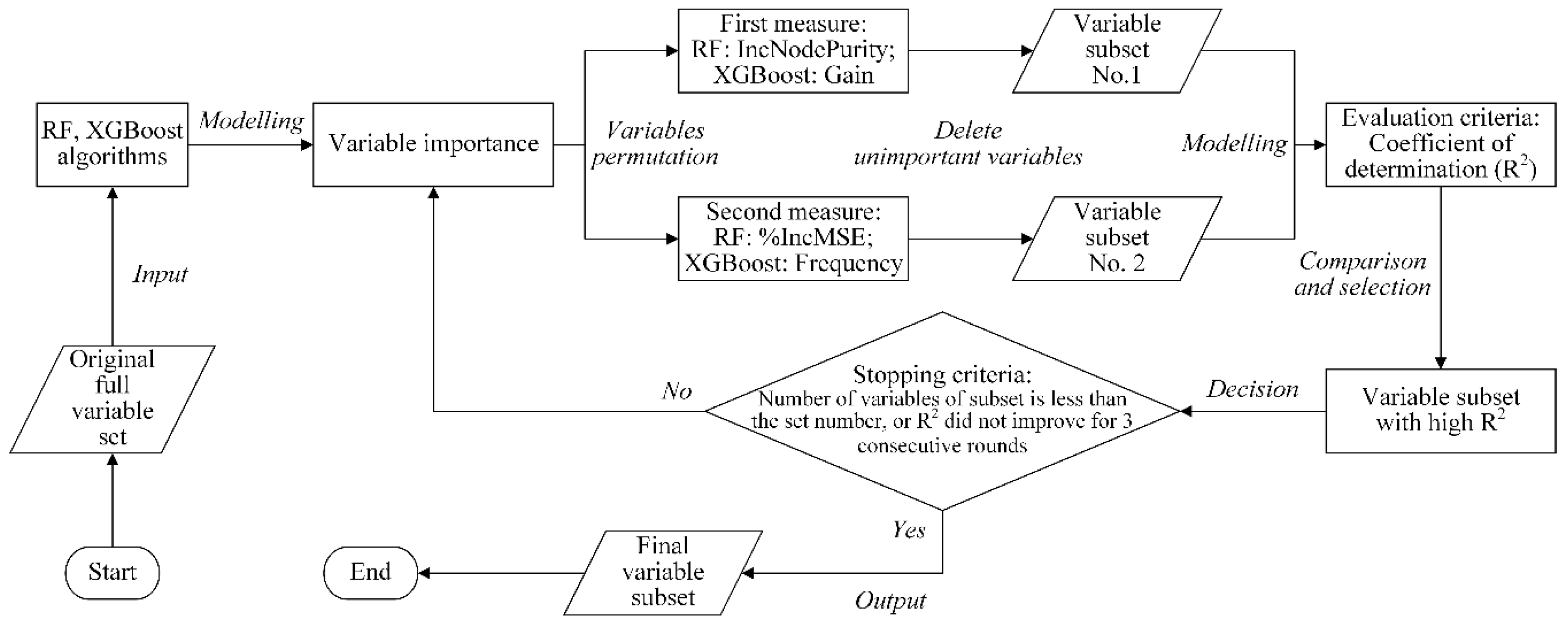
25]. Variable selection (also known as feature selection) can select a most effective variable subset from the full variable set to reduce variable space dimension, and improve the generalization and intelligibility of the model [26]. Variable selection is one of the most important steps in AGB modeling. Stepwise regression, which is the most commonly used method of variable selection of linear regression model, is simple and easy to perform [27]. Many variable selection algorithms (such as the random forest algorithm) include variable ranking based on some evaluation strategies as a principal or auxiliary selection mechanism because of their simplicity, scalability, and good empirical success [28,29].
In addition to variable selection, it is crucial to select a suitable algorithm to establish AGB estimation models. The traditional statistical regression algorithm, which can build a linear relationship between forest AGB and remote sensing data, is simple and easy to calculate. One of the traditional regression algorithms, the linear regression (LR) method was the most widely used method for AGB estimation in the previous studies [9,30]. However, the traditional statistical regression method cannot effectively express the complex relationship between forest AGB and remote sensing data under an indeterminate distribution of data. Therefore, the machine learning algorithms, such as K-nearest neighbor (KNN), support vector machine, artificial neural network, and decision tree, are applied to the remote sensing-based AGB estimation for improving the nonlinear estimation ability of the biomass model [31,32,33,34]. Previous studies have indicated that algorithms based on the decision tree, such as random forest (RF) and gradient boosting (GB), have an excellent performance in biomass estimation [35,36]. The RF is not only a variable selection algorithm but is also used as a nonlinear regression algorithm for AGB estimation because of its advantages of fewer adjustable parameters, high speed and efficiency, and the ability of variable importance calculation and permutation [37,38]. The extreme gradient boosting (XGBoost), as an advanced GB system, is widely used by data scientists and has provided state-of-the-art results for many fields, especially the financial field, such as credit risk assessment [39], but its potential has not been fully utilized in forestry.
The importance of field investigation for remote sensing-based AGB modeling is self-evident. Since 1973, China has conducted a continuous forest inventory, and in this process has established a comprehensive database covering many aspects of forest resources, involving forest health, timber production, and forest ecosystem services. The National Forest Continuous Inventory (NFCI), which is the first level of the forest inventory system of China, was designed to provide reliable data of the current status of and changes in the forests in the form of an integrated spatial database [40]. The NFCI survey is carried out every five years at the provincial scale. The sample plots have been systematically located at the graticule intersection of the national topographic map (scale of 1:100,000 or 1:50,000) [41]. Each tree with a diameter at breast height greater than or equal to 5 cm in the sample plot was tagged and permanently numbered for remeasurement in subsequent inventory periods. The NFCI is important for the formulation and refinement of state forest planning, management, and policy [42]. Therefore, the NFCI was widely used in many studies, including assessment and monitoring of forest status, conditions and changes, carbon sink and source identification, biomass estimation, and biodiversity [30,43].
In this paper, we used the NFCI data and Landsat 8 Operational Land Imager (OLI) data in combination with the LR and two machine learning algorithms, e.g., RF and XGBoost, to establish models for AGB estimation under the condition of known forest types and then created the AGB map for the study area using the optimal models. The specific objectives of this study were as follows: (1) to explore the influence of variable selection for the LR, RF, and XGBoost; (2) to validate the ability of the RF and XGBoost for estimating AGB; (3) to compare the accuracy of the LR, RF, and XGBoost models of different forest types; and (4) to draw the AGB map for the study area.

2. Study Area

Hunan Province (21.18 × 10⁴ km2, 24°38′ N–30°08′ N, 108°47′ E–114°15′ E) is situated in the south-central region of China (Figure 1). Most of the study areas are located in a subtropical monsoon humid climate zone, and the annual average temperature, rainfall, and sunshine duration are 14.80–18.50 °C, 1200–1800 mm, and 1238.7–1868.7 h, respectively. Therefore, the abundant resources of sunlight, water, and heat, with rain and heat over the same period, can promote the rapid growth of trees and enhance the ability of natural regeneration. The forestland area is 13.00 × 10⁴ km2, accounting for 61.37% of the study area; its forest coverage is 59.68%, and the total standing forest stock is 5.48 × 10⁸ m3 [44]; it is one of the key forest areas and major timber production bases in Southern China.

3. Data

3.1. Inventory Data

The eighth NFCI data of Hunan Province, which were surveyed in 2014, were used in this study. The size of each square plot is 25.82 × 25.82 m (approximately 0.0667 ha), and the plots were systematically allocated based on a grid of 4 km × 8 km. Note that the plots, which were situated on non-forestry land (such as cropland, water area, urban land, and bare land), or were covered by cloud in the remote sensing images, were eliminated. Finally, 3886 plots, which recorded around 149,000 trees, were used for modeling in this study (Figure 1).
The AGB of a tree was calculated by using the general one-variable aboveground biomass model, which can be expressed as [45]:
M a =   a × D 7 / 3
a = 0.3 × p
where M a (kg) is the AGB of a tree, D (cm) is the diameter at breast height, a is the parameter of a tree species, and p (g/cm3) is the basic wood density (Table A1). The plot AGB was converted to per hectare biomass (Mg/ha).
The plots were classified into three types, namely coniferous, broadleaf, and mixed forest, based on the species standing volume according to the technical regulation for forest continuous inventory of China (Table 1). In general, the average AGB of all plots with non-classification of forest types (abbreviated as “All” in all tables and figures) was 50.06 Mg/ha, within the range of 5.48–268.60 Mg/ha, with a standard deviation of 35.34 Mg/ha; the average AGB values of coniferous, broadleaf, and mixed forest were 48.71, 46.63, and 59.43 Mg/ha, respectively (Table 2).
Compared with the digital elevation model, the high value of AGB is mainly distributed in the southeastern and western regions with a high altitude and steep slope and has a high vegetation coverage, low population density, less human interference, and poor economic condition. By contrast, the low value of AGB is mainly distributed in the low hills and valleys, with a low altitude and gentle slope; the conditions are opposite, especially in the middle region, which is the valley of Xiangjiang River with many towns and villages, and cropland. The spatial distribution trend of AGB is consistent with the topographic features and socio-economic conditions of the study area.

3.2. Landsat 8 Data

The Landsat Surface Reflectance products, which were derived from Landsat 8 OLI satellite images, were used in this study. The images, which were acquired in October 2015, were downloaded from the United States Geological Survey (USGS) website (https://earthexplorer.usgs.gov/, accessed on 20 October 2019). There were 30 screen images (Figure 1).
Radiometric and atmospheric correction of the Landsat Surface Reflectance images was performed by USGS [46]. For the areas of complex topography and with a great difference in elevation, terrain correction can effectively eliminate the shadow of the terrain as well as the difference in spectral features between a sunny slope and a shaded slope due to the topographic relief, preferably reflecting the true spectral feature of the object [47]. The terrain correction used the C-correction algorithm [48]. Then, the images were resampled to a pixel size of 25.82 m, the same as the inventory plot. The texture images were calculated using a grey-level co-occurrence matrix algorithm with 3 × 3, 5 × 5, and 7 × 7-pixel windows [49]. In addition, 20 vegetation indices were generated for this study (Appendix A). Landsat 8 OLI data were processed by the Environment for Visualizing Images software (Version 5.3.1, Boulder, CO, USA).
Finally, the remote sensing predictor variables, which were extracted for each plot center, included the primal images of 6 Landsat Surface Reflectance band images as well as the generated images of 20 vegetation index images and 144 texture images (Table 3).

3.3. Land Cover Image

The European Space Agency (ESA) Climate Change Initiative (CCI) project, of which the objective is to realize the full potential of the long-term global earth observation archives as a significant and timely contribution to the Essential Climate Variables databases required by United Nations Framework Convention on Climate Change, delivered consistent global Land Cover (LC) maps at a 300 m spatial resolution on an annual basis from 1992 to 2015 [50]. There is a highly positive result of the accuracy of the different classes: the highest user accuracy values are found for the classes of cropland (0.89–0.92), broadleaf forest (0.94–0.96), urban areas (0.86–0.88), bare (0.86–0.88), water bodies (0.92–0.96), and permanent snow and ice (0.96–0.97); the mixed and coniferous forest has a relatively low user accuracy value with 0.79–0.81 and 0.82–0.83, respectively [50]. The CCI-LC map for 2014 was downloaded from the ESA website (http://maps.elie.ucl.ac.be/CCI/viewer/index.php, accessed on 20 October 2019) for this study.
The typology of CCI-LC was defined using the Land Cover Classification System developed by the Food and Agriculture Organization of the United Nations, Rome, Italy. The map was consolidated into seven types based on the typology of CCI-LC: coniferous, broadleaf, and mixed forests, cropland, urban, water, and other types (non-forestry land, included bare land, grassland, etc.) (Figure 2). Then, the CCI-LC map was resampled to 25.82 m and snapped to the grid of Landsat 8 images.
For validation of the accuracy and consistency of classification between NFCI and CCI-LC, the attribute of the CCI-LC map was extracted by the NFCI plot center. The result indicated that the producer accuracies of the CCI-LC map of coniferous, broadleaf, and mixed forests were 0.91, 0.88, and 0.82, respectively, and the user accuracies were 0.93, 0.91, and 0.92, respectively; the overall accuracy and kappa coefficient of coniferous, broadleaf and mixed forests were 0.92 and 0.88, respectively (Table 4). Therefore, the classified accuracy of the CCI-LC map can satisfy the research needs of this paper.

4. Methods

4.1. Algorithms of AGB Estimation

4.1.1. Linear Regression

The LR can quantitatively describe the correlation and significance between variables. The LR, which assumes a linear relationship between a response and a set of explanatory variables, can be expressed by the following model [30]:
Y = α 0 + α 1 X 1 + α 2 X 2 + + α n X n + ε
where Y is the value of AGB, X 1 , X 2 , …, X n are the predictor variables, α 0 is a constant, α 1 , α 2 , …, α n are the regression coefficients associated with the corresponding variables, n is the number of the predictor variables, and ε is the error term.

4.1.2. Random Forest

Decision trees are popular because they represent information in a way that is intuitive and easy to visualize and also have several other advantageous properties. The RF and XGBoost models, two ensemble techniques that combine the separate decision tree models to improve the ability of models, were considered in this paper.
RF is a classification and regression algorithm based on decision tree proposed by Breiman [51] in 2001. RF is one of the most common approaches to capture the complex relationship between a response and a set of explanatory variables with the following advantages: robustness to reduce over-fitting, ability to determine variable importance, higher accuracy, fewer parameters that need to be tuned, lower sensitivity to tuning of the parameters, fast training speed, and anti-noise property [25].
RF randomly collects a new dataset from the original sample dataset by bootstrapping. Generally, about 2/3 of the original sample data are selected in one bootstrap sample, and the remaining 1/3 of the data are used as out-of-bag data. Then, each bootstrap sample is used to establish a corresponding decision tree and combines multiple trees to improve the prediction performance [51]. When RF was used for regression, the mean of all decision tree prediction results was taken as the final prediction result. RF has been applied extensively as a classification algorithm [52] and has been used for time series forecasting in large-scale regression-based spatial applications [25,53].

4.1.3. Extreme Gradient Boosting

XGBoost, which was proposed by Chen et al. [54] and is very popular in data mining and machine learning competitions all over the world, is an improved gradient boosting decision tree (GBDT). Compared with the GBDT, XGBoost performs a second-order Taylor expansion for the objective function and uses the second derivative to accelerate the convergence speed of the model while training [55]. Unlike the independent decision trees of RF, XGBoost can correct the residual error to generate a new tree based on the previous tree [56].
The advantages of XGBoost include [54]:
(1)
Using the second-order Taylor expression for the objective function, making the definition of the objective function more precise, and the optimal solution can be easily found;
(2)
The addition of a regularization term into the objective function to control the complexity of the tree to obtain a simple model and to avoid overfitting;
(3)
The use of sampling of the column feature to reduce the calculation amount and prevent overfitting; and
(4)
The use of an effective cache-aware block structure for out-of-core tree learning to parallel and distributed computing makes learning faster for hundreds of millions of examples.
Generally, XGBoost is a highly scalable tree structure enhanced model, which can handle sparse and missing data well and can greatly improve the speed of the algorithm and compress computational memory in large-scale data training.

4.2. Methods of Variable Selection

Variable selection is the process of selecting the minimal and most effective variable subset from the original variable set to reduce the dimension of variable space and maximize the evaluation criteria [29]. Generally, the variable selection algorithm should determine four elements as follows: search starting point and direction, search strategy, evaluation function, and stopping criterion [57], but the algorithms mainly focus on the search strategy and evaluation function. In this paper, the stepwise regression approach was used to select the variable for LR, and the variable importance-based method was used for RF and XGBoost.

4.2.1. Stepwise Regression Approach

Stepwise regression is an important analysis method in LR analysis, which is mainly used to solve the problem of how to select explanatory variables when the number of explanatory variables is too many in the LR model so that all explanatory variables significantly impact the response variable in the regression equation [27]. Stepwise regression is used to introduce the explanatory variables one by one into the regression equation according to the contribution for the response variable. An introduced explanatory variable will be removed from the regression equation if it becomes non-significant due to the introduction of the subsequent new explanatory variable. After each explanatory variable is introduced or excluded, the F-test based on the sum of squares of partial regression is performed to ensure that only significant explanatory variables are included in the regression equation. This process is repeated until no non-significant explanatory variables are selected in the regression equation and no significant explanatory variables are removed from the regression equation to ensure that the final set of explanatory variables is optimal.
In this paper, stepwise regression was performed in SPSS software (Version 25, Armonk, NY, USA), and the probability of the F-test was set to 0.05 and 0.10 for entry and removal, respectively.

4.2.2. Variable Importance-Based Method

Each RF and XGBoost algorithm define two measures for variable importance, which can be used to rank variables. For RF, the first measure, which is computed from permuting out-of-bag data, is the percent increase in the mean square error (%IncMSE) of the prediction for each tree, and the second measure is the total decrease in node impurities (IncNodePurity) from splitting on the variable averaged over all trees, which is measured by the residual sum of squares [58]. Higher %IncMSE and IncNodePurity values indicate a more important predictor variable. For XGBoost, the first measure is calculated by the fractional contribution (Gain) of each feature to the model based on the total gain of this variable’s splits, and the second measure is calculated by the relative number (Frequency) of times a feature be used in trees [59]. A higher percentage of Gain and Frequency means a more important predictor variable.
The acquisition of the optimal variable subset is a continuous search process, which would generally include four steps [60]:
(1) Subset generation: generate a candidate variable subset according to a certain search strategy. In this paper, the generalized sequential backward selection approach was used. The start point of the search is the original full variable set. The dataset was input into the RF and XGBoost models to obtain the variable importance and descending order, respectively, according to the measures. Then, a certain number (10%) of variables, which were the most unimportant, were removed to generate a variable subset.
(2) Subset evaluation: evaluate the prediction performance of the variable subset through an evaluation function. The generated subset was input into RF and XGBoost models, and the prediction accuracy was evaluated using the coefficient of determination (R2). In this paper, there were two evaluation results in each round, so the corresponding variable subset with high R2 was compared and then selected as the selected variable subset in this round.
(3) Stopping criterion: determine when the variable search algorithm should stop. After the subset evaluation, the stopping criterion should be determined. If there is no stopping criterion, the search process cannot be stopped. In this paper, two stopping criteria were set: first if the number of variables of the subset was not larger than the set number, which was equal to the number of selected variables by stepwise regression for different forest types; and, second, if the R2 of the prediction of the subset did not improve for three consecutive rounds.
(4) Subset validation: used to verify the validity of the selected variable subset. In this paper, a 10-fold cross-validation approach was performed to evaluate the performance of the variable subset in each round; therefore, the subset validation was not an independent step in the process.
In this paper, the modeling and variable selection of RF and XGBoost were implemented by the R packages randomForest [58] and xgboost [59], respectively. The workflow of variable selection is shown in Figure 3.

4.3. Variable Interactions

The two-way interactions between predictor variables graphically using the three-dimensional partial dependence plot, which was presented by Elith et al. [61], were used in this paper. In these plots, two of the predictor variables from the model, which are plotted on the x and y axes, are used to produce a grid of possible combinations of predictor variable values over the range of both variables, and the remaining predictor variables from the model are fixed at either their means (for continuous predictors) or their most common value (for categorical predictors). Model predictions are generated over this grid and plotted as the z-axis. The “model.interaction.plot” function of the R package ModelMap develops these plots, which can work with both continuous and categorical predictor variables [62].

4.4. Evaluation of AGB Models

The correlation test between the predictor variables and AGB was performed using the Pearson correlation coefficient in SPSS Statistics software.
In addition to the coefficient of determination (R2), the root-mean-square error (RMSE) and the percentage root-mean-square error (RMSE%) were also used to evaluate the performance of the final models:
R 2 = 1 i = 1 n ( y i y ^ i ) 2 / i = 1 n ( y i y ¯ i ) 2
R M S E = i = 1 n ( y i y ^ i ) 2 / n
R M S E % = R M S E y ¯ × 100
where y i is the observed AGB value, y ^ i is the predicted AGB value based on models, y ¯ is the arithmetic mean of all the observed AGB values, and n is the sample number. In general, a higher R2 value and lower RMSE and RMSE% values indicate a better estimation performance of the model.
In addition, the difference of prediction between LR, RF, and XGBoost for different forest types was evaluated using the F-test.

5. Results

5.1. Role of Predictor Variables

5.1.1. Variable Importance

The result of the Pearson correlation coefficients between the predictor variables and AGB indicated that 144 variables had a significance level of 0.01 with the AGB, and the texture image variables had a significant correlation with the AGB. The variable with the highest correlation coefficient was B4T7Mea, with a value of −0.42.
Twenty-nine LR models were established using the selected predictor variables by stepwise regression for three forest types (i.e., coniferous, broadleaf, and mixed forest) and all plots with non-classification of forest types (Table 5). The results indicated that the performance of the models was improved when the count of predictor variables increased, and the models of different forest types worked better than the models of all forest plots (R2 values of models for the coniferous, broadleaf, mixed, and all forest plots were 0.32, 0.37, 0.34, and 0.30, respectively).
The four best models (i.e., model numbers 7, 15, 21, and 29) were selected as the base to compare the performance of other types of models for the coniferous, broadleaf, and mixed forest (Table 6). The predictor variables of the LR models were different, and the collinearity statistics of the predictor variables were less than 5.50, which showed that the selected variables were effective. The predictor variables of these models were dominated by the image texture information. The standardized coefficients and the significance levels of the models showed that the texture-type variables contributed more than other variable types, which indicated that the texture variables were very important for the AGB estimation using the LR model in this study.
Figure 4 shows the selected predictor variables based on variable importance for the different forest types of RF and XGBoost models. The predictor variables of the RF and XGB models were not similar, and the main variables were the texture variables; the correlation and mean were included in all models, which indicated that the texture images had sufficient information to enhance the performance of models for AGB estimation. The texture of bands 5, 7, or both with a 7 × 7-pixel window were frequently involved in the models, indicating the significant roles of these two band texture variables in AGB estimation.
However, the selected variables were different for the different forest types. The spectral bands, vegetation indices, and texture variables played a significant role in the broadleaf, mixed, and coniferous forest RF models, respectively. The species and canopy layers of broadleaf and mixed forests were multiple, which could be expressed by abundant spectral information; thus, the spectral and vegetation index variables could account sufficiently for the AGB estimation; the species composition of the coniferous forest was relatively single, which mainly consisted of fir and pine, and there was no obvious difference in the spectrum, whereas the texture information could well explain the AGB estimation [24,63]. This phenomenon of variable selection is more obvious in RF models than in XGBoost models. Unlike RF models, besides the texture variables, the spectral variables were also important for XGBoost models; especially Band4, which was the most important variable in all XGBoost models. Previous studies have shown that Band4, where the chlorophylls have peak absorption, had a strong relationship with biomass [64].
In addition, the relationship between the selected predictor variables was calculated using the Pearson correlation coefficient. We found that RF models mostly split the importance among the correlated multiple variables, whereas XGBoost models are inclined to centralize the importance at a single variable. For example, Band4 was significantly correlated with VARI at a significance level of 0.01 with a value of −0.77; they had a similar importance in the RF model, but the importance was concentrated on Band2 in the XGBoost model for the coniferous forest. This conclusion is the same as that reported by Freeman et al. [65].

5.1.2. Variable Interactions

The result indicated, surprisingly, that Band4, VARI, or both were involved in almost models, especially in XGBoost models (Figure 4). Figure 5 shows how Band4 and VARI interact for the AGB estimation of the XGBoost models. We did not find significant interaction effects in these models, but we did find subtle interactions. These figures show that Band4 mainly affected the interval with a low value (<300), but the effect of VARI was different. For the model of the coniferous forest, the high values of predicted AGB were mainly concentrated in the interval with a low value of VARI (<0.0), and there were some significant differences with the adjacent interval. In contrast, the high values of predicted AGB were dispersed in all intervals of VARI with a low interval of Band4, but there were hardly any high values in other intervals for the model of the broadleaf forest. However, the effects of VARI and Band4 for the mixed forest model were significantly different from the models of the coniferous and broadleaf forests. Although the high values of predicted AGB were also concentrated in the interval with high values of VARI (>0.4), there were many higher values of predicted AGB that were distributed in other intervals of Band4. For the model of all forest plots, the effect of Band4 and VARI was more similar to the combination of the models of coniferous, broadleaf, and mixed forests.
The interaction plots examine the effects of the two predictor variables with the remaining variables fixed at their mean value for continuous predictors (or the most common value for categorical predictors). The plots illustrated that they were seemingly more dependent on VARI than Band4 in these two-way interactions, although Band4 was the most important predictor in the estimation models. Compared with the model of all forest plots, each model of the coniferous, broadleaf, and mixed forests has distinct characteristics, which is beneficial for establishing AGB models with a high accuracy.

5.1.3. Performance of Variable Selection

The forward selection approach, which increases variables step-by-step, was used in stepwise regression; whereas the backward selection approach, which deletes variables step-by-step, was used in the variable selection of RF and XGBoost models. For the LR models, the performance of the models was improved when the number of predictor variables increased (Table 5).
Figure 6 illustrates how the R2 values change with the number of selected variables for RF and XGBoost models. Each line represents an independent model, and the different colors indicate the different forest types. The result indicated that the R2 values of models increased when the number of predictor variables decreased. Generally, the most dramatic change was the line of the mixed forest, followed by the lines of coniferous and broadleaf forests, whereas the line of all forest plots exhibited the smallest change in both RF and XGBoost models, although the variation degree of each line was different between RF and XGBoost models.
Contrasting the lines of the two algorithms, besides that the performance of XGBoost was better than that of RF, the influence of the number of predictor variables on the performance of models was also different. For RF, the influence of the number of predictor variables was relatively low, which manifested in a smooth change of the lines, whereas the influence was dramatic for XGBoost, with jagged peaks and valleys of the lines. This also indicated the variable selection was more important for XGBoost than for RF.

5.2. Evaluation of AGB Models

After the variable selection, we obtained the 12 best models of LR, RF, and XGBoost for different forest types. The performance of models was expressed by scatterplots, which showed the relationship between the predicted AGB values and observed AGB values (Figure 7). The plots showed that the RF model worked better than the LR model, and the XGBoost model worked better than the RF model for the same forest type. The results also indicated that the model of the broadleaf forest had the highest accuracy, followed by the models of mixed and coniferous forests, whereas the performance of the model for all forest plots was the worst for the same algorithm.
We found that problems of underestimation and overestimation, which also existed in the previous studies, were experienced by all models [30,66,67]. Intuitively, the predicted value was higher than the centerline when the biomass was low but lower when it was high in the figures. This means that the problem of overestimation and underestimation of remote sensing AGB estimation had no a fundamental solution, although the performance of models had a significant improvement based on forest type.
To further verify whether the models differed significantly, the F-test was used (Figure 8). The confidence level was set at 95%. In Figure 8, the numbers are the p-values, which are from the F-test, and the color of the checkerboard shows the levels of significance. The F-test results showed that there were significant differences of the predicted AGB between the LR, RF, and XGBoost models at a confidence level of 95%, although the p-values were different for these models (especially the p-value of all forest plots, which was higher than that of the other models).

5.3. Mapping AGB

Finally, we drew the two AGB maps for the study area using the XGBoost models: first by estimating the AGB of the coniferous, broadleaf, and mixed forests according to the forest types in Figure 2, then combining these into one map (Figure 9a); second by estimating the AGB using all plots with non-classification of forest types (Figure 9b).
In Figure 9, two maps of AGB had a similar trend in spatial distribution, which is consistent with the AGB distribution trend of the inventory plots in Figure 1. The results indicated that the ranges of predicted AGB for the two maps were different. The values ranged from 3.10 to 235.50 Mg/ha with a mean of 53.84 Mg/ha for the AGB map based on the forest type (Figure 9a), and the distribution and range of values were in close proximity to the inventory values in Figure 1. However, the range of values was from 6.50 to 210.30 Mg/ha with a mean of 52.39 Mg/ha for the AGB map based on all plots with non-classification of forest type (Figure 9b). In addition, the values of AGB in Figure 9a were higher than those in Figure 9b in the same area with a high value and were lower in the same area with a low value. This indicated that the ability of AGB estimation based on forest type was clearly improved for the high and low values. This improvement is also what we expected.
The degrees of overestimation and underestimation of the two maps were different, although the problems of overestimation and underestimation still existed. To further verify this conclusion, we sorted the values of the predicted AGB into three ranges based on the distribution of values: low (3 < predicted AGB < 25), medium (25 ≤ predicted AGB < 65), and high (65 ≤ predicted AGB < 236) values (Figure 10). The corresponding values of predicted AGB for the two maps and the AGB difference (Figure 9a minus Figure 9b) were obtained by the overlaying operations. In the low range of predicted AGB, most of the values of AGB prediction based on forest types (abbreviated as “Classification” in Figure 10) were lower than the values of AGB prediction of all plots with non-classification of forest type (abbreviated as “Non-classification” in Figure 10), and the values of the difference were mainly distributed from −10 to 2 Mg/ha (Figure 10a); therefore, the “Classification” map had a better prediction performance. In the medium range, the distribution of the AGB difference approximated a normal distribution, indicating that two maps had a similar performance for medium values of AGB (Figure 10b). In the high range, the values of “Classification” were clearly higher than those for “Non-classification”, indicating that the “Classification” map also had better performance with respect to the high AGB values (Figure 10c). In summary, the map, which was predicted based on forest type, better estimated the AGB value than the map with the non-classification of forest type irrespective of high or low AGB.

6. Discussion

Through this experiment, we increased our understanding of the importance of variable selection, which can influence the performance of machine learning algorithms. Variable selection is one of the most important processes in modeling, which can reduce data dimension and the storage space of data, speed the estimation process, and improve the interpretability and performance of models [29].
Multiple predictor variables, such as spectral bands, vegetation indices, and textures, were extracted from remote sensing images and were used for modeling AGB in this paper. However, these predictors cannot all be used for modeling due to their high correlations and high numbers. The performance of models was significantly impacted by the number of selected predictor variables (Figure 6, Table 5). Through the variable selection, the number of predictor variables was reduced from hundreds to several, which makes it easier to interpret the model. In this study, the Red (Band4), NIR (Band5), SWIR (Band7) bands, and the derived variables played a more important role than other bands. In models of AGB estimation, the SWIR band is more sensitive to the shadow of vegetation and humidity of soil and is less influenced by the atmospheric conditions [16,22,68]; the NIR band of Landsat 8, of which the wavelength range was adjusted to 0.845–0.885 µm to exclude the effect of water-vapor absorption at 0.825 µm, is more sensitive to vegetation of different types [13,69]; and the red band is usually used to distinguish the vegetation type [21,64,70]. We cannot ignore the fact that the vegetation index variables were also selected frequently, especially VARI, which exists in all XGBoost models. Compared with other vegetation indices, VARI is minimally sensitive to the atmospheric effect, and the estimation error of vegetation affected by the atmosphere is less than 10% in a large area [71,72].
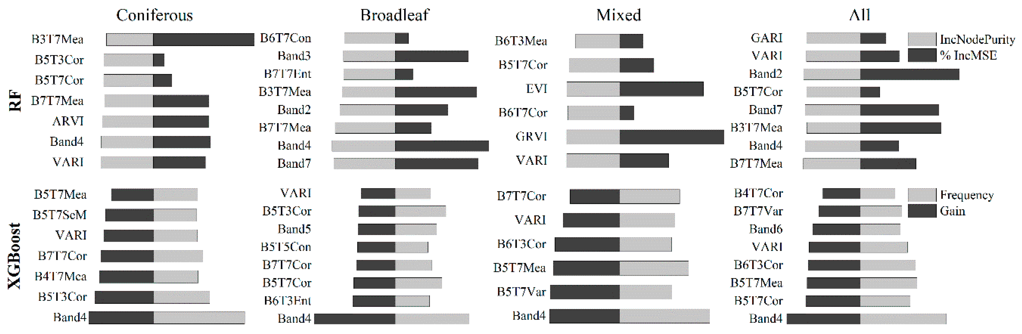
In addition, the textures, which are dominant in all models, were also critical for AGB estimation, although the importance of the texture predictor variables was different from that in previous studies [24,30,66]. However, for the different forest types, texture variables and spectral variables played different roles in AGB models (Figure 4). For example, the spectral variables were more important than texture variables in the RF model of the broadleaf forest, while the texture variables were more important in the RF model of the coniferous forest. This illustrated that the role of texture variables and spectral variables was dependent on forest structure: in the broadleaf and mixed forest with multiple species and complex structure, the models tended to select the spectral variables, while in the coniferous forest with relatively fewer species and simple structure, the models tended to choose texture variables [63,64,73].
Due to the different characters between spectral variables and texture variables, their combination is beneficial to improve the performance of AGB models, and this improvement was evident in all models. Moreover, the influence of variable selection was different for RF and XGBoost. We found that the accuracy of the XGBoost algorithm varied greatly with the number of selected variables compared with RF (Figure 6). The RF algorithm can be regarded as a parallel ensemble algorithm because the decision tree of RF is independent; thus, RF is not sensitive to inclusion of the noisy predictor variables [74,75], whereas the decision tree of XGBoost is generated based on the previous tree; thus, the noisy predictor variables will influence the accuracy of the subsequent new tree [76,77].
The LR algorithm, which assumes a linear relationship between predictor and predicted variables, was used frequently in most early biomass estimation studies due to the interpretability of LR [30,78]. However, the relationship between remote sensing data and AGB is complex; thus, the traditional statistical regression algorithm cannot efficiently describe the relationship between them. Therefore, machine learning algorithms such as random forest and gradient boosting, which can establish a complex non-linear relationship between vegetation information and remote sensing images with an indeterminate distribution of data, were introduced to improve the accuracy of AGB estimation [79].
In our study, we extracted 170 predictor variables from Landsat 8 images; then, a few variables were selected from these through the variable selection process to build RF and XGBoost models (Figure 4). We found that the machine learning algorithms prevented overfitting and significantly improved the estimation accuracy compared with the LR models, and the result also indicated that the XGBoost model worked better than the RF model (Figure 7). The XGBoost algorithm, which is a highly flexible algorithm with the ability to correct the residual error to generate a new tree based on the previous tree, provided an improvement in processing a regularized learning objective to avoid overfitting [54].
Before this study, few studies had used the XGBoost algorithm to estimate AGB. Li et al. [30] used a linear mixed-effects model and linear dummy variable model to estimate AGB in the western Hunan Province of China; the R2 values of total vegetation were 0.41; Zhu et al. [6] used multiple algorithms (LR, KNN, logistic regression) to estimate AGB for the Xiangjiang River, and the results indicated the machine learning algorithm had a good performance for AGB estimation. In contrast, the results obtained by machine learning methods in this study were better, and the XGBoost algorithm had a good performance in AGB estimation and could reduce underestimation and overestimation to some extent.
In this paper, we established the models based on forest type to improve the accuracy of AGB estimation, and the results indicated this method was valuable. We found that the models based on forest type had a better performance at the lower and higher values compared to the models of all plots with non-classification of forest types, especially XGBoost (Figure 7 and Figure 9). In addition, the problem of overestimation and underestimation, which are the main factors influencing AGB modeling performance, was not completely solved, although the performance of models had a significant improvement compared with the previous studies. As to this problem, it is decided by the algorithm itself on one hand. The decision trees, which are the key components of the RF and XGBoost methods, cannot extrapolate outside the training set. On the other hand, it is related to the remote sensing data. For plots with low AGB values, the shrubs, grass, and bare soil will influence the reflectance of bands; the pixel of Landsat 8 with relatively low spatial resolution (30 × 30 m) is a mixed pixel, which cannot accurately express the spectral information of land cover. For plots with high AGB values, the saturation in multispectral sensors such as Landsat 8 OLI is the main reason for underestimation of AGB [80,81]. Therefore, remote sensing data with higher spatial and radiometric resolution such as LIDAR data and hyperspectral data, or the approach of mixed pixel decomposition, may be solutions for AGB estimation. Meanwhile, a modeling approach based on the AGB range may be a useful method for improving the prediction of AGB, but it needs more sample plots.
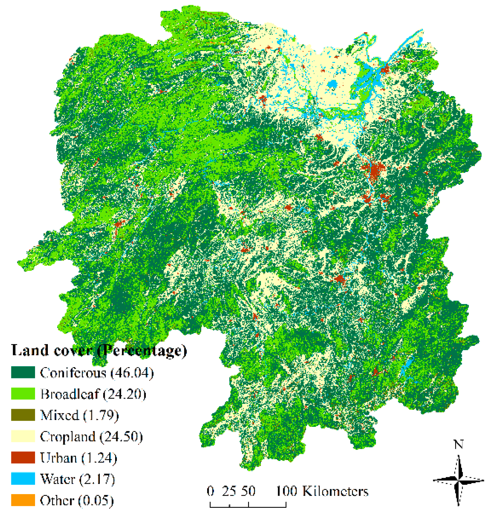
The subtropical forests of China are distributed in 13 provinces, including Zhejiang, Jiangsu, Anhui, Fujian, Jiangxi, Hubei, Hunan, Guangdong, Guangxi, Hainan, Guizhou, Sichuan, and Yunnan. They are one of the dominant distribution areas of forest resources in China. It is necessary to monitor the subtropical forest change because the forests have been influenced by the improved silviculture, woody encroachment, climate change, and human activities. The forest biomass estimation based on traditional field measurements is a relatively accurate method, but it is impossible to implement for such large areas of subtropical forests. Therefore, remote sensing-based estimation of forest biomass change is a very important method. The NFCI data, which has been checked and revised many times by the state and provincial forest departments before it is released, is the only available data with highest quality in the provincial scale at present. However, the residual atmospheric effects and calibration errors in satellite data cannot be completely eliminated. Therefore, until the more effective satellite data are available, we can only hope to improve the accuracy of forest biomass estimation by using new modeling methods. Despite certain inaccuracies, the performance of the biomass estimation method used in this study exceeds our expectations, and the selected modeling method of XGBoost seems to be more effective. The results show that the NFCI data in combination with Landsat 8 can be successfully applied to biomass estimation. Although the XGBoost models had the relatively high RMSE and RMSE% values, the total accuracies of models were significantly increased with the variable selection, and it is still manifested that the methods in this paper were very important and useful for the provincial-scale accurate estimation of forest biomass, and these methods can also be used to other similar areas. In addition, we must admit that there are still many sections that could be improved in our research, such as methods of variable selection, variable data cleaning, and parameter optimization for machine learning. We will do further research in these aspects in the future.

7. Conclusions

In this study, we selected the subtropical region of Hunan Province, China, as a case study area to analyze the AGB estimation based on forest type using different modeling algorithms, namely, LR, RF, and XGBoost. The results indicated the following: (1) Variable selection is a very important part of machine learning algorithms. In this study, variable selection had a significant effect on the performance of XGBoost compared with that of RF. (2) Machine learning algorithms have advantages in AGB estimation. In this paper, the XGBoost and RF models significantly improved the estimation accuracy compared with the LR models, and the XGBoost algorithm reduced overestimation and underestimation to a certain extent, although the problem was not fully eliminated. (3) The method of AGB estimation based on forest type is a very useful approach to improve the accuracy of AGB estimation, and the models had a better performance at the lower and higher values compared with the models using all plots with non-classification of forest types. In this paper, we provided a new approach when establishing similar models. The result and conclusion may be different for other areas, but we hope to pay attention to variable selection when using machine learning algorithms in the future and will try to use various remote sensing data and algorithms to improve the accuracy of biomass estimation.

Author Contributions

Y.L. and M.L.; data curation: Y.L., C.L., and Z.L.; formal analysis: Y.L., C.L., and Z.L.; funding acquisition: M.L.; methodology: Y.L. and M.L.; project administration: M.L.; resources: M.L.; software: Y.L., and C.L.; supervision: M.L.; validation: Y.L., C.L., and Z.L.; visualization: Y.L. and Z.L.; writing—original draft: Y.L.; writing—review and editing: Y.L., M.L., C.L., and Z.L.

Acknowledgments

This study was financially supported by the National Natural Science Foundation of China (no. 31770679), and Top-notch Academic Programs Project of Jiangsu Higher Education Institutions, China (TAPP, PPZY2015A062). The authors would like to thank our editors, as well as the anonymous reviewers for their valuable comments, and also LetPub (www.letpub.com) for linguistic assistance during the preparation of this manuscript.

Conflicts of Interest

The authors declare no conflict of interest.

Appendix A

Table A1. The wood density of the tree species or groups.
Tree Species/GroupsWood Density (p)Tree Species/GroupsWood Density (p)
Abies0.3464Pinus massoniana0.4476
Betula0.4848Pinus tabulaeformis0.4243
Cinnamomum0.4600Pinus taiwanensis0.4510
Cryptomeria0.3493Pinus yunnanensis0.3499
Cunninghamia lanceolata0.3098Populus0.4177
Cupressus0.5970Quercus0.5762
Eucalyptus0.5820Robinia pseudoacacia0.6740
Fraxinus mandshurica0.4640Salix0.4410
Larix0.4059Schima superba0.5563
Liquidambar formosana0.5035Tilia0.3200
Paulownia0.2370Ulmus0.4580
Picea0.3730Other conifers0.3940
Pinus armandii0.3930Other pines0.4500
Pinus densata0.4720Other hardwood broadleaves0.6250
Pinus elliottii0.4118Other softwood broadleaves0.4430
Note: The total relative error of the tree species or groups was 2.10%, not exceeding the common allowance of 3%, and the average of the absolute relative error was 6.37%, less than the error allowance of 10% [45].

References

  1. Brown, S. Measuring carbon in forests: Current status and future challenges. Environ. Pollut. 2002, 116, 363–372. [Google Scholar] [CrossRef]
  2. Gower, S.T. Patterns and mechanisms of the forest carbon cycle. Annu. Rev. Environ. Resour. 2003, 28, 169–204. [Google Scholar] [CrossRef]
  3. Houghton, R.A. Aboveground forest biomass and the global carbon balance. Glob. Chang. Biol. 2005, 11, 945–958. [Google Scholar] [CrossRef]
  4. Houghton, R.A.; Hall, F.; Goetz, S.J. Importance of biomass in the global carbon cycle. J. Geophys. Res. Biogeosci. 2009, 114, 1–13. [Google Scholar] [CrossRef]
  5. Lu, D.; Batistella, M.; Moran, E. Satellite estimation of aboveground biomass and impacts of forest stand structure. Photogramm. Eng. Remote Sens. 2005, 71, 967–974. [Google Scholar] [CrossRef]
  6. Zhu, J.; Huang, Z.; Sun, H.; Wang, G. Mapping forest ecosystem biomass density for xiangjiang river basin by combining plot and remote sensing data and comparing spatial extrapolation methods. Remote Sens. 2017, 9, 241. [Google Scholar] [CrossRef]
  7. West, P.W. Tree and Forest Measurement, 3rd ed.; Springer: Berlin/Heidelberg, Germany, 2015; ISBN 978-3-319-14707-9. [Google Scholar]
  8. Crosby, M.K.; Matney, T.G.; Schultz, E.B.; Evans, D.L.; Grebner, D.L.; Londo, H.A.; Rodgers, J.C.; Collins, C.A. Consequences of landsat image strata classification errors on bias and variance of inventory estimates: A forest inventory case study. IEEE J. Sel. Top. Appl. Earth Obs. Remote Sens. 2017, 10, 243–251. [Google Scholar] [CrossRef]
  9. Lu, D. The potential and challenge of remote sensing-based biomass estimation. Int. J. Remote Sens. 2006, 27, 1297–1328. [Google Scholar] [CrossRef]
  10. Avitabile, V.; Herold, M.; Heuvelink, G.B.M.; Simon, L.; Phillips, O.L.; Asner, G.P.; Armston, J.; Peter, S.; Banin, L.; Bayol, N.; et al. An integrated pan-tropical biomass map using multiple reference datasets. Glob. Chang. Biol. 2016, 22, 1406–1420. [Google Scholar] [CrossRef]
  11. Deng, S.; Katoh, M.; Guan, Q.; Yin, N.; Li, M. Estimating forest aboveground biomass by combining ALOS PALSAR and WorldView-2 data: A case study at Purple Mountain National Park, Nanjing, China. Remote Sens. 2014, 6, 7878–7910. [Google Scholar] [CrossRef]
  12. Cao, L.; Coops, N.C.; Innes, J.L.; Sheppard, S.R.J.; Fu, L.; Ruan, H.; She, G. Estimation of forest biomass dynamics in subtropical forests using multi-temporal airborne LiDAR data. Remote Sens. Environ. 2016, 178, 158–171. [Google Scholar] [CrossRef]
  13. Loveland, T.R.; Irons, J.R. Landsat 8: The plans, the reality, and the legacy. Remote Sens. Environ. 2016, 185, 1–6. [Google Scholar] [CrossRef]
  14. Wulder, M.A.; Loveland, T.R.; Roy, D.P.; Crawford, C.J.; Masek, J.G.; Woodcock, C.E.; Allen, R.G.; Anderson, M.C.; Belward, A.S.; Cohen, W.B.; et al. Current status of Landsat program, science, and applications. Remote Sens. Environ. 2019, 225, 127–147. [Google Scholar] [CrossRef]
  15. Loveland, T.R.; Dwyer, J.L. Landsat: Building a strong future. Remote Sens. Environ. 2012, 122, 22–29. [Google Scholar] [CrossRef]
  16. Roy, D.P.; Wulder, M.A.; Loveland, T.R.; Woodcock, C.E.; Allen, R.G.; Anderso, M.C.; Helder, D.; Irons, J.R.; Johnson, D.M.; Kennedy, R.; et al. Landsat-8: Science and product vision for terrestrial global change research. Remote Sens. Environ. 2014, 145, 154–172. [Google Scholar] [CrossRef]
  17. Wulder, M.A.; White, J.C.; Cranny, M.; Hall, R.J.; Luther, J.E.; Beaudoin, A.; Goodenough, D.G.; Dechka, J.A. Monitoring Canada’s forests. Part 1: Completion of the EOSD land cover project. Can. J. Remote Sens. 2008, 34, 549–562. [Google Scholar] [CrossRef]
  18. Lehmann, E.A.; Wallace, J.F.; Caccetta, P.A.; Furby, S.L.; Zdunic, K. Forest cover trends from time series Landsat data for the Australian continent. Int. J. Appl. Earth Obs. Geoinf. 2013, 21, 453–462. [Google Scholar] [CrossRef]
  19. Shimabukuro, Y.E.; Batista, G.T.; Mello, E.M.K.; Moreira, J.C.; Duarte, V. Using shade fraction image segmentation to evaluate deforestation in landsat thematic mapper images of the Amazon Region. Int. J. Remote Sens. 1998, 19, 535–541. [Google Scholar] [CrossRef]
  20. Banskota, A.; Kayastha, N.; Falkowski, M.J.; Wulder, M.A.; Froese, R.E.; White, J.C. Forest monitoring using landsat time series data: A review. Can. J. Remote Sens. 2014, 40, 362–384. [Google Scholar] [CrossRef]
  21. Chrysafis, I.; Mallinis, G.; Gitas, I.; Tsakiri-Strati, M. Estimating Mediterranean forest parameters using multi seasonal Landsat 8 OLI imagery and an ensemble learning method. Remote Sens. Environ. 2017, 199, 154–166. [Google Scholar] [CrossRef]
  22. Lu, D. Aboveground biomass estimation using Landsat TM data in the Brazilian Amazon. Int. J. Remote Sens. 2005, 26, 2509–2525. [Google Scholar] [CrossRef]
  23. Ouma, Y.O. Optimization of second-order grey-level texture in high-resolution imagery for statistical estimation of above-ground biomass. J. Environ. Inf. 2006, 8, 70–85. [Google Scholar] [CrossRef]
  24. Lu, D.; Batistella, M. Exploring TM image texture and its relationships with biomass estimation in Rondônia, Brazilian Amazon. Acta Amaz. 2005, 35, 249–257. [Google Scholar] [CrossRef]
  25. Shen, W.; Li, M.; Huang, C.; Tao, X.; Wei, A. Annual forest aboveground biomass changes mapped using ICESat/GLAS measurements, historical inventory data, and time-series optical and radar imagery for Guangdong province, China. Agric. For. Meteorol. 2018, 259, 23–38. [Google Scholar] [CrossRef]
  26. Yu, K.; Wu, X.; Ding, W.; Pei, J. Scalable and accurate online feature selection for big data. ACM Trans. Knowl. Discov. Data 2016, 11, 1–39. [Google Scholar] [CrossRef]
  27. Wang, Y.; Wen, L.; Chen, M. Dictionary of Mathematics, 5th ed.; Science Press: Beijing, China, 2017; ISBN 9787030533364. [Google Scholar]
  28. Genuer, R.; Poggi, J.M.; Tuleau-Malot, C. Variable selection using random forests. Pattern Recognit. Lett. 2010, 31, 2225–2236. [Google Scholar] [CrossRef]
  29. Bolón-Canedo, V.; Sánchez-Maroño, N.; Alonso-Betanzos, A. Feature selection for high-dimensional data. Prog. Artif. Intell. 2016, 5, 65–75. [Google Scholar] [CrossRef]
  30. Li, C.; Li, Y.; Li, M. Improving forest aboveground biomass (AGB) estimation by incorporating crown density and using landsat 8 OLI images of a subtropical forest in Western Hunan in Central China. Forests 2019, 10, 104. [Google Scholar] [CrossRef]
  31. Reese, H.; Nilsson, M.; Sandstro, P. Applications using estimates of forest parameters derived from satellite and forest inventory data. Comput. Electron. Agric. 2002, 37, 37–55. [Google Scholar] [CrossRef]
  32. Baccini, A.; Laporte, N.; Goetz, S.J.; Sun, M.; Dong, H. A first map of tropical Africa’s above-ground biomass derived from satellite imagery. Environ. Res. Lett. 2008, 3, 1–9. [Google Scholar] [CrossRef]
  33. Nelson, R.; Montesano, P.; Ranson, K.J.; Kharuk, V.; Sun, G.; Kimes, D.S. Estimating Siberian timber volume using MODIS and ICESat/GLAS. Remote Sens. Environ. 2009, 113, 691–701. [Google Scholar] [CrossRef]
  34. Monnet, J.-M.; Chanussot, J.; Berger, F. Support vector regression for the estimation of forest stand parameters using airborne laser scanning. IEEE Geosci. Remote Sens. Lett. 2011, 8, 580–584. [Google Scholar] [CrossRef] [Green Version]
  35. Blackard, J.A.; Finco, M.V.; Helmer, E.H.; Holden, G.R.; Hoppus, M.L.; Jacobs, D.M.; Lister, A.J.; Moisen, G.G.; Nelson, M.D.; Riemann, R.; et al. Mapping U.S. forest biomass using nationwide forest inventory data and moderate resolution information. Remote Sens. Environ. 2008, 112, 1658–1677. [Google Scholar] [CrossRef]
  36. Carreiras, J.M.B.; Vasconcelos, M.J.; Lucas, R.M. Understanding the relationship between aboveground biomass and ALOS PALSAR data in the forests of Guinea-Bissau (West Africa). Remote Sens. Environ. 2012, 121, 426–442. [Google Scholar] [CrossRef]
  37. Karlson, M.; Ostwald, M.; Reese, H.; Sanou, J.; Tankoano, B.; Mattsson, E. Mapping tree canopy cover and aboveground biomass in sudano-sahelian woodlands using landsat 8 and random forest. Remote Sens. 2015, 7, 10017–10041. [Google Scholar] [CrossRef] [Green Version]
  38. Zald, H.S.J.; Wulder, M.A.; White, J.C.; Hilker, T.; Hermosilla, T.; Hobart, G.W.; Coops, N.C. Integrating landsat pixel composites and change metrics with lidar plots to predictively map forest structure and aboveground biomass in Saskatchewan, Canada. Remote Sens. Environ. 2016, 176, 188–201. [Google Scholar] [CrossRef] [Green Version]
  39. Carmona, P.; Climent, F.; Momparler, A. Predicting failure in the U.S. banking sector: An extreme gradient boosting approach. Int. Rev. Econ. Financ. 2019, 61, 304–323. [Google Scholar] [CrossRef]
  40. Lei, X.; Tang, M.; Lu, Y.; Hong, L.; Tian, D. Forest inventory in China: Status and challenges. Int. For. Rev. 2009, 11, 52–63. [Google Scholar] [CrossRef]
  41. Zeng, W.; Tomppo, E.; Healey, S.P.; Gadow, K.V. The national forest inventory in China: History—Results—International context. For. Ecosyst. 2015, 2, 23. [Google Scholar] [CrossRef] [Green Version]
  42. Xie, X.; Wang, Q.; Dai, L.; Su, D.; Wang, X.; Qi, G.; Ye, Y. Application of China’s National Forest Continuous Inventory Database. Environ. Manage. 2011, 48, 1095–1106. [Google Scholar] [CrossRef]
  43. Fang, J.; Chen, A.; Peng, C.; Zhao, S.; Ci, L. Changes in forest biomass carbon storage in China between 1949 and 1998. Science 2001, 292, 2320–2322. [Google Scholar] [CrossRef]
  44. Hunan Provincial People’s Government Natural Resources of Hunan Province. Available online: http://www.enghunan.gov.cn/AboutHunan/HunanFacts/NaturalResources/201507/t20150707_1792317.html (accessed on 1 November 2019).
  45. Zeng, W. Developing one-variable individual tree biomass models based on wood density for 34 tree species in China. For. Res. Open Access 2018, 7, 1–5. [Google Scholar]
  46. USGS Landsat Surface Reflectance Data. Available online: https://pubs.usgs.gov/fs/2015/3034/pdf/fs20153034.pdf (accessed on 27 March 2019).
  47. Richter, R. Correction of Atmospheric and Topographic Effects for High Spatial Resolution Satellite Imagery. Int. J. Remote Sens. 1997, 18, 1099–1111. [Google Scholar] [CrossRef]
  48. Teillet, P.M.; Guindon, B.; Goodenough, D.G. On the slope-aspect correction of multispectral scanner data. Can. J. Remote Sens. 1982, 8, 84–106. [Google Scholar] [CrossRef] [Green Version]
  49. Haralick, R.M.; Shanmugam, K.; Dinstein, I. Textural features for image classification. IEEE Trans. Syst. Man. Cybern. 1973, SMC-3, 610–621. [Google Scholar] [CrossRef] [Green Version]
  50. ESA Land Cover CCI Product User Guide. Available online: http://maps.elie.ucl.ac.be/CCI/viewer/download/ESACCI-LC-Ph2-PUGv2_2.0.pdf (accessed on 10 April 2017).
  51. Breiman, L. Random forest. Mach. Learn. 2001, 45, 5–32. [Google Scholar] [CrossRef] [Green Version]
  52. Yu, Y.; Li, M.; Fu, Y. Forest type identification by random forest classification combined with SPOT and multitemporal SAR data. J. For. Res. 2018, 29, 1407–1414. [Google Scholar] [CrossRef]
  53. Tyralis, H.; Papacharalampous, G.; Tantanee, S. How to explain and predict the shape parameter of the generalized extreme value distribution of streamflow extremes using a big dataset. J. Hydrol. 2019, 574, 628–645. [Google Scholar] [CrossRef]
  54. Chen, T.; Guestrin, C. XGBoost: A Scalable Tree Boosting System. In Proceedings of the 22nd ACM SIGKDD International Conference on Knowledge Discovery and Data Mining (KDD ’16), San Francisco, CA, USA, 13–17 August 2016; pp. 785–794. [Google Scholar]
  55. He, H.; Zhang, W.; Zhang, S. A novel ensemble method for credit scoring: Adaption of different imbalance ratios. Expert Syst. Appl. 2018, 98, 105–117. [Google Scholar] [CrossRef]
  56. Friedman, J.H. Stochastic gradient boosting. Comput. Stat. Data Anal. 2002, 38, 367–378. [Google Scholar] [CrossRef]
  57. Guyon, I.; Andre, E. An introduction to variable and feature selection. J. Mach. Learn. Res. 2003, 3, 1157–1182. [Google Scholar]
  58. Liaw, A.; Wiener, M. RandomForest: Breiman and Cutler’s Random Forests for Classification and Regression. Available online: https://cran.r-project.org/package=randomForest (accessed on 25 March 2018).
  59. Chen, T.; He, T.; Benesty, M.; Khotilovich, V.; Tang, Y. xgboost: Extreme Gradient Boosting. Available online: https://cran.r-project.org/package=xgboost (accessed on 1 August 2019).
  60. Dash, M.; Liu, H. Feature selection for classification. Intell. Data Anal. 1997, 1, 131–156. [Google Scholar] [CrossRef]
  61. Elith, J.; Leathwick, J.R.; Hastie, T. A working guide to boosted regression trees. J. Anim. Ecol. 2008, 77, 802–813. [Google Scholar] [CrossRef]
  62. Freeman, E.; Frescino, T. ModelMap: Modeling and Map Production Using Random Forest and Related Stochastic Models. Available online: https://cran.r-project.org/web/packages/ModelMap/index.html (accessed on 11 September 2018).
  63. Suganuma, H.; Abe, Y.; Taniguchi, M.; Tanouchi, H.; Utsugi, H.; Kojima, T.; Yamada, K. Stand biomass estimation method by canopy coverage for application to remote sensing in an arid area of Western Australia. For. Ecol. Manag. 2006, 222, 75–87. [Google Scholar] [CrossRef]
  64. Lu, D.; Chen, Q.; Wang, G.; Liu, L.; Li, G.; Moran, E. A survey of remote sensing-based aboveground biomass estimation methods in forest ecosystems. Int. J. Digit. Earth 2016, 9, 63–105. [Google Scholar] [CrossRef]
  65. Freeman, E.A.; Moisen, G.G.; Coulston, J.W.; Wilson, B.T. Random forests and stochastic gradient boosting for predicting tree canopy cover: Comparing tuning processes and model performance. Can. J. For. Res. 2016, 46, 323–339. [Google Scholar] [CrossRef] [Green Version]
  66. Gao, Y.; Lu, D.; Li, G.; Wang, G.; Chen, Q.; Liu, L.; Li, D. Comparative analysis of modeling algorithms for forest aboveground biomass estimation in a subtropical region. Remote Sens. 2018, 10, 627. [Google Scholar] [CrossRef] [Green Version]
  67. Kajisa, T.; Murakami, T.; Mizoue, N.; Kitahara, F.; Yoshida, S. Estimation of stand volumes using the k-nearest neighbors method in Kyushu, Japan. J. For. Res. 2008, 13, 249–254. [Google Scholar] [CrossRef]
  68. Ustin, S.L.; Roberts, D.A.; Gamon, J.A.; Asner, G.P.; Green, R.O. Using imaging spectroscopy to study ecosystem processes and properties. Bioscience 2004, 54, 523. [Google Scholar] [CrossRef]
  69. USGS Landsat 8 (L8) Data Users Handbook. Available online: https://prd-wret.s3-us-west-2.amazonaws.com/assets/palladium/production/atoms/files/LSDS-1574_L8_Data_Users_Handbook_v4.pdf (accessed on 20 September 2004).
  70. Barsi, J.; Lee, K.; Kvaran, G.; Markham, B.; Pedelty, J. The spectral response of the Landsat-8 operational land imager. Remote Sens. 2014, 6, 10232–10251. [Google Scholar] [CrossRef] [Green Version]
  71. Gitelson, A.A.; Stark, R.; Grits, U.; Rundquist, D.; Kaufman, Y.; Derry, D. Vegetation and soil lines in visible spectral space: A concept and technique for remote estimation of vegetation fraction. Int. J. Remote Sens. 2002, 23, 2537–2562. [Google Scholar] [CrossRef]
  72. Gitelson, A.A.; Kaufman, Y.J.; Stark, R.; Rundquist, D. Novel algorithms for remote estimation of vegetation fraction. Remote Sens. Environ. 2002, 80, 76–87. [Google Scholar] [CrossRef] [Green Version]
  73. Kelsey, K.; Neff, J. Estimates of aboveground biomass from texture analysis of landsat imagery. Remote Sens. 2014, 6, 6407–6422. [Google Scholar] [CrossRef] [Green Version]
  74. Dietterich, T.G. An experimental comparison of three methods for constructing ensembles of decision trees. Mach. Learn. 2000, 40, 139–157. [Google Scholar] [CrossRef]
  75. Díaz-Uriarte, R.; Alvarez de Andrés, S. Gene selection and classification of microarray data using random forest. BMC Bioinf. 2006, 7, 1–13. [Google Scholar] [CrossRef] [Green Version]
  76. Sheridan, R.P.; Wang, W.M.; Liaw, A.; Ma, J.; Gifford, E.M. Extreme gradient boosting as a method for quantitative structure—Activity relationships. J. Chem. Inf. Model. 2016, 56, 2353–2360. [Google Scholar] [CrossRef]
  77. Georganos, S.; Grippa, T.; Vanhuysse, S.; Lennert, M.; Shimoni, M.; Wolff, E. Very high resolution object-based land use–land cover urban classification using extreme gradient boosting. IEEE Geosci. Remote Sens. Lett. 2018, 15, 607–611. [Google Scholar] [CrossRef]
  78. Dong, J.; Kaufmann, R.K.; Myneni, R.B.; Tucker, C.J.; Kauppi, P.E.; Liski, J.; Buermann, W.; Alexeyev, V.; Hughes, M.K. Remote sensing estimates of boreal and temperate forest woody biomass: Carbon pools, sources, and sinks. Remote Sens. Environ. 2003, 84, 393–410. [Google Scholar] [CrossRef] [Green Version]
  79. Ali, I.; Greifeneder, F.; Stamenkovic, J.; Neumann, M.; Notarnicola, C. Review of machine learning approaches for biomass and soil moisture retrievals from remote sensing data. Remote Sens. 2015, 7, 16398–16421. [Google Scholar] [CrossRef] [Green Version]
  80. Moghaddam, M.; Dungan, J.L.; Acker, S. Forest variable estimation from fusion of SAR and multispectral optical data. IEEE Trans. Geosci. Remote Sens. 2002, 40, 2176–2187. [Google Scholar] [CrossRef]
  81. Mutanga, O.; Skidmore, A.K. Narrow band vegetation indices overcome the saturation problem in biomass estimation. Int. J. Remote Sens. 2004, 25, 3999–4014. [Google Scholar] [CrossRef]
Figure 1. The location of the study area, including the forest types and observed AGB of the field plots, and the Landsat 8 scene numbers (P: path, R: row).
Forests 10 01073 g001
Figure 2. Classification of CCI-LC for the study area.
Forests 10 01073 g002
Figure 3. Workflow of the variable selection based on variable importance for RF and XGBoost models.
Forests 10 01073 g003
Figure 4. Variable importance of RF and XGBoost based on different forest types. The variable importance of each model was scaled to sum to 1.
Forests 10 01073 g004
Figure 5. Interaction plots for VARI and Band4 for the XGBoost models based on different forest types.
Forests 10 01073 g005
Figure 6. The accuracy of RF and XGBoost models with the selected variable number changing based on different forest types.
Forests 10 01073 g006
Figure 7. Scatter plot of the predicted and observed AGB of the LR, RF, and XGBoost models based on different forest types.
Forests 10 01073 g007
Figure 8. The comparisons (F-test) of the LR, RF, and XGBoost models based on forest type. The labels of the vertical and horizontal axes represent the models using a different algorithm. XGB represents the XGBoost model.
Forests 10 01073 g008
Figure 9. The predicted AGB using XGBoost models based on the different forest types, including (a) AGB map based on forest type and (b) AGB map based on all plots with non-classification of forest type.
Forests 10 01073 g009
Figure 10. Histograms illustrating the difference in pixel number in three ranges. Note that the vertical axis labels represent the range of the prediction difference between two AGB maps (Figure 9a minus Figure 9b); Classification: values from Figure 10a, Non-classification: values from Figure 9b. (a) 3 < Predicted AGB ≤ 25, (b) 25 ≤ Predicted AGB < 65, (c) 65 ≤ Predicted AGB < 236.
Forests 10 01073 g010
Table 1. Classification standard of forest types.
Forest TypeStandard of Division
ConiferousPure coniferous forest (single coniferous species stand volume ≥ 65%)
Coniferous mixed forest (coniferous species total stand volume ≥ 65%)
BroadleafPure broadleaf forest (single broad-leaved species stand volume ≥ 65%)
broadleaf mixed forest (broad-leaved species total stand volume ≥ 65%)
MixedBroadleaf-coniferous mixed forest (total stand volume of coniferous or broad-leaved species accounting for 35%–65%)
Table 2. Distribution of the plot AGB values (Mg/ha) of the different forest types.
Forest TypeCountMinimumMaximumMeanStandard DeviationPercentage of Different AGB Range (%)
5–3030–6060–9090–120120–270
Coniferous18397.68223.1248.7126.5727.9045.6219.035.222.23
Broadleaf15355.48268.6046.6343.8144.3626.7814.077.627.17
Mixed51218.60219.9559.4334.2120.3138.8724.619.386.84
All38865.48268.6050.0635.3433.4037.2917.816.724.79
Table 3. Summary of predictor variables including Landsat Surface Reflectance band images, vegetation indices, and texture images for AGB estimation.
Variable TypeVariables NumberVariable NameDescription
Band Image6Band2, Band3, Band4, Band5, Band6, Band7Landsat 8 Bands 2–7:
Blue, Green, Red, NIR, SWIR1, SWIR2
Vegetation Index20ARVIAtmospherically Resistant Vegetation Index
DVIDifference Vegetation Index
EVIEnhanced Vegetation Index
GARIGreen Atmospherically Resistant Index
GDVIGreen Difference Vegetation Index
GNDVIGreen Normalized Difference Vegetation Index
GRVIGreen Ratio Vegetation Index
GVIGreen Vegetation Index
IPVIInfrared Percentage Vegetation Index
LAILeaf Area Index
MNLVIModified Non-Linear Vegetation Index
MSRVIModified Simple Ratio Vegetation Index
NDVINormalized Difference Vegetation Index
NLVINon-Linear Vegetation Index
OSAVIOptimized Soil Adjusted Vegetation Index
RDVIRenormalized Difference Vegetation Index
RVIRatio Vegetation Index
SAVISoil Adjusted Vegetation Index
TDVITransformed Difference Vegetation Index
VARIVisible Atmospherically Resistant Index
Texture Image144BiTjCon, BiTjDis, BiTjMea, BiTjHom, BiTjSeM, BiTjEnt, BiTjVar, BiTjCorLandsat bands 2–7 texture measurement using gray-level co-occurrence matrix
Note: BiTjXXX represents a texture image developed in the Landsat Surface Reflectance band i (2–7) using the texture measure XXX with a j × j (3, 5, 7) pixel window, where XXX is Con (contrast), Dis (dissimilarity), Mea (mean), Hom (homogeneity), SeM (angular second moment), Ent (entropy), Var (variance), or Cor (correlation).
Table 4. Confusion matrix of classification between CCI-LC and NFCI.
Forest TypeClassification of CCI-LCProducer Accuracy
ConiferousBroadleafMixedCroplandUrbanWaterOther
Classification based on NFCI dataConiferous164976332973110.91
Broadleaf621150205346140.88
Mixed5443627312570.82
User Accuracy0.930.910.92
Table 5. Performance of LR models based on stepwise regression of different forest types.
Forest TypeModel No.Count of VariablesR2RMSERMSE%Forest TypeModel No.Count of VariablesR2RMSERMSE%
Coniferous110.2834.2470.29Mixed1610.2335.4259.6
220.2932.6467.01 1720.2833.0955.68
330.331.163.85 1830.330.9452.06
440.3130.7963.21 1940.3230.2550.9
550.3230.5962.8 2050.3330.0150.5
660.3230.2662.12 2160.3429.6549.89
770.3230.1661.92
Broadleaf810.3230.4765.34All2210.2634.5769.06
920.3429.7363.76 2320.2734.3368.58
1030.3429.8764.06 2430.2834.268.32
1140.3528.9262.02 2540.2833.4466.8
1250.3528.3160.71 2650.2932.6165.14
1360.3627.9759.98 2760.2931.963.72
1470.3627.5659.1 2870.2931.4862.88
1580.3727.3258.59 2980.331.1262.17
Table 6. The predictor variable selection and estimation of the highest accuracy of LR models (Model Nos. 7, 15, 21, and 29 in Table 5) of different forest types.
Forest TypePredictor VariableStandardized CoefficientsEstimate (t-Test)Significance (p-Value)Collinearity StatisticsForest TypePredictor VariableStandardized CoefficientsEstimate (t-Test)Significance (p-Value)Collinearity Statistics
ConiferousB4T7Mea−0.20−6.7401.66MixedSAVI0.224.2401.41
B5T7Cor−0.10−4.0601.11 B3T7Cor0.143.1301.08
B7T5Cor0.072.80.011.15 B7T3Dis0.112.240.031.38
B4T3Ent−0.19−3.8204.69 B6T3Cor0.12.310.021.08
B4T5Hom−0.13−2.590.014.96 B5T3Con0.162.540.012.18
B3T7Cor0.052.10.041.06 B5T7Hom0.131.890.052.44
GVI−0.05−2.010.051.31
BroadleafB5T7Mea−0.13−3.0603.11AllB4T7Mea−0.14−4.2504.62
LAI0.297.2602.63 B3T7Cor0.084.801.04
B3T7Cor0.072.9701.02 B4T7SeM0.042.230.031.49
B4T7SeM0.32.8705.14 B5T7Mea−0.07−2.420.023.4
B4T5SeM−0.25−2.420.023.82 LAI0.184.8205.37
B7T3Mea0.182.8104.99 B7T3Mea0.13.6603.4
B6T7Mea−0.14−2.020.042.52 GDVI−0.08−2.170.035.15
B6T3Var−0.05−1.830.051.09 B5T7Cor−0.03−1.970.051.03

