Article

Forest-Type Classification Using Time-Weighted Dynamic Time Warping Analysis in Mountain Areas: A Case Study in Southern China

1
State Key Laboratory of Resources and Environmental Information System, Institute of Geographic Sciences and Natural Resources Research, Chinese Academy of Sciences, Beijing 10010, China
2
University of Chinese Academy of Sciences, Beijing 10010, China
3
Jiangsu Center for Collaborative Innovation in Geographical Information Resource Development and Application, Nanjing 210023, China
*
Author to whom correspondence should be addressed.
Forests 2019, 10(11), 1040; https://doi.org/10.3390/f10111040
Submission received: 9 October 2019 / Revised: 7 November 2019 / Accepted: 14 November 2019 / Published: 16 November 2019

Abstract

:
Efficient methodologies for mapping forest types in complicated mountain areas are essential for the implementation of sustainable forest management practices and monitoring. Existing solutions dedicated to forest-type mapping are primarily focused on supervised machine learning algorithms (MLAs) using remote sensing time-series images. However, MLAs are challenged by complex and problematic forest type compositions, lack of training data, loss of temporal data caused by clouds obscuration, and selection of input feature sets for mountainous areas. The time-weighted dynamic time warping (TWDTW) is a supervised classifier, an adaptation of the dynamic time warping method for time series analysis for land cover classification. This study evaluates the performance of the TWDTW method that uses a combination of Sentinel-2 and Landsat-8 time-series images when applied to complicated mountain forest-type classifications in southern China with complex topographic conditions and forest-type compositions. The classification outputs were compared to those produced by MLAs, including random forest (RF) and support vector machine (SVM). The results presented that the three forest-type maps obtained by TWDTW, RF, and SVM have high consistency in spatial distribution. TWDTW outperformed SVM and RF with mean overall accuracy and mean kappa coefficient of 93.81% and 0.93, respectively, followed by RF and SVM. Compared with MLAs, TWDTW method achieved the higher classification accuracy than RF and SVM, with even less training data. This proved the robustness and less sensitivities to training samples of the TWDTW method when applied to mountain forest-type classifications.

1. Introduction

Mountain forests are vital for preventing soil erosion, protecting crops from wind and cold air, and protecting settlements, roads, and farmland from landslides, avalanches, and floods [1]. Recently, because of human activities, natural disasters, and climate change, different types of forests have been destroyed at different degrees. Accurate forest-type maps are critical for monitoring and managing forest resources in various regions [2,3]. For mountain areas, it is complicated to obtain the spatial distribution and quantity information of forest types through human investigation due to complex forest compositions and topographic conditions. Remote sensing technology provides unprecedented support for forest-type mapping [4]. However, terrain fluctuations, cloud occlusions, and a lack of reference data further increase the difficulty of forest-type classification in mountainous areas using remote sensing technology [5]. Therefore, it is necessary to explore effective methods to extract explicit and detailed information of forest types in complex mountain areas.
Since the 1970s, many studies have been focused on how remote sensing could contribute to forest mapping [6,7,8,9,10,11,12,13,14,15,16,17,18,19,20]. However, owing to the unique geographical environments and biological distribution characteristics of forests, the “same object different spectrum” and “different object same spectrum” phenomena generally exist in forest vegetation, which further complicate the application of remote sensing for forest-type classification [21]. Scholars have proposed various solutions, among of them, there is evidence that time-series data offer improvements over forest-type mapping in complex and mountainous areas. For example, Grabska et al. [22] produced a forest stand species map for the northern part of the Carpathian Mountains using Sentinel-2 time-series data and confirmed that using these data rather than single-data significantly improved forest-species mapping. Pasquarella et al. [23] classified forest types for western Massachusetts with complex topography using the Landsat time-series data, verifying that using time-series data outperformed individual data or multi-date combinations. Zhu and Liu [24] mapped detailed forest types using dense Landsat time series and revealed that using Landsat time series can significantly improve the accuracy of forest-type mapping compared with a single image. Cheng et al. [25] took Qinling Mountains in China as an example, and proved the potential application of Sentinel-2 time series data for forest-type classification.
Regarding classification algorithms, non-parametric classifiers, such as machine-learning algorithms (MLAs), have been proven to perform well in forest-type classifications in mountainous areas because they can accurately classify natural land cover types [26,27]. The assumption that the data are normally distributed is not necessary with MLAs, which makes it possible to include non-spectral ancillary data in the classification process [28]. Therefore, there are forest cover studies for mountain regions that have used MLAs, such as supervised decision trees [29], logistic regression [30], maximum likelihood [31], spectral unmixing [32], and random forest (RF) [33]. Of these MLAs, RF is an exceptionally flexible ensemble learning method that has been gaining attention in forest-type classifications [34]. Because RF can effectively handle high-dimensional, noisy, and multi-source datasets without over-fitting and achieve higher classification accuracy than other well-known classifiers, such as support vector machines (SVM) and maximum likelihood [33,34,35,36]. However, forest-type mapping based on these methods is challenged by the (1) lack of samples used to train the supervised algorithm, especially for inaccessible steep mountainous areas; (2) dimensionality problems caused by a large input feature set; (3) loss of temporal data caused by cloud obscuration; and (4) change in phenological cycles caused by climate variations in a mountainous area.
Dynamic time warping (DTW) [37] has been recognized as an efficient solution to handle above challenges [38,39]. Maus et al. [40] proposed a time-weighted version of the DTW method (TWDTW) capable of classifying crops with various vegetation dynamics. TWDTW analysis was also proved an effective method in identifying a single forest and pasture from the enhanced vegetation index (EVI) derived from MODIS data [40]. However, for forest-type classification in mountain areas, the performance of the TWDTW algorithm and its comparison with other MLAs have not been explored. The objective of this study is to evaluate the performance of TWDTW and MLAs for forest-type classifications in mountainous regions with complex topography based on available Sentinel-2 and Landsat-8 time-series images. Specifically, the performances of the TWDTW, RF, and SVM methods and their sensitivities to the number of training data have been evaluated for mountain regions with complex topographies located in southern China.

2. Materials and Methods

2.1. Study Area

The study area is situated in Hunan Province of southern China, at 26°40′2″ N–27°9′13″ N, 109°26′00″ E–110°8′40″ E (Figure 1), covering 3810.63 km2 with a complex mountain topography. There are various landforms, such as mountain plains, hills, ridges, and synclinal valleys. The elevation is between 200 m and 2000 m, and the topographic slope generally ranges from 36° to 50°, the maximum of which reached 60°, forming a complex terrain with thousands of peaks and gullies, most of which are steep slopes and cliffs above 45° [41]. The area belongs to a humid subtropical mountain climate with average annual temperatures between 14.2 °C and 16.4 °C and average annual precipitation of 1365.9 mm. The three-dimensional climate features in the study area are evident, and the microclimate effect is significant. The region contains one of the most abundant forest resources in Hunan Province and has various forest types (e.g., fruit forests, oil-yielding trees, and Chinese fir plantations, among others). The area is also the transition zone from the evergreen broad-leaved forests in the hilly mountains of eastern China to the dark coniferous forests in the northwestern alpine plateau.

2.2. Data Sets

2.2.1. Remote Sensing Images

The images used include Sentinel-2 and Landsat-8 time-series data. All images were selected from 2016 to 2018 with <10% cloud cover. For Sentinel-2, the top of atmosphere (TOA) reflectance satellite data were selected, and the input bands included Band1 (coastal aerosol), QA60, blue, green, red, near-infrared, and bitmask (containing cloud mask information) bands. For Landsat-8, the surface reflectance products were used directly, and the input bands included the pixel quality attributes, blue, green, red, and near-infrared bands.

2.2.2. Training and Validation Samples

Reference samples were acquired from a forest inventory map produced in 2008 from the China Forest Science Data Center (CFSDC) (http://www.cfsdc.org/), which was created by artificial investigation and could represent ground truth [4]. In order to determine whether the forest type in the study area has been changed, firstly, a Google Earth Engine-based implementation of the Continuous Degradation Detection (CODED) algorithm [42] was used to identify stable area based on the Landsat data. Then reference samples were manually outlined from the unchanged area in forest inventory map. Therefore, the samples extracted basically can be regarded as ground truth information [4]. The reference data were divided into two parts based on the polygon IDs for training and validation, respectively, and 50% of the reference data were randomly selected from each class as training data, while the remaining data were used for accuracy validation. We use ArcGIS 10.4 software to convert polygons into points to form the training and verification data set. The number of samples for training and validation is listed in Table 1.

2.3. Methodology

The methodological workflow (Figure 2) consisted of the following steps: (1) preprocessing, which involved the identification and masking of clouds, cirrus, and aerosols [25], image composition, and Normalized Difference Vegetation Index (NDVI) time-series creation; (2) classification in which TWDTW, RF, and SVM were used to map the target classes; and (3) comparison and evaluation in which the forest-type maps obtained by TWDTW, RF, and SVM were compared in terms of spatial identification and quantity, and the classification accuracy of each method was assessed.

2.3.1. Preprocessing

The preprocessing step consisted of three parts, which were all processed in Google Earth Engine (GEE) using Javascript:
  • Cloud mask. For Landsat-8, “cloud shadows” (bit 3), “clouds” (bit 5), medium–high “cloud confidence” (bits 6–7), and medium–high “cirrus confidence” (Landsat-8 only, bits 8–9) were masked using the pixel quality attributes band. For Sentinel, Sentinel-2 Band QA60 was used to identify and mask flagged cloud and cirrus pixels. The remaining cloud and aerosols were then identified using an aerosol band (Band 1) and were likewise masked. The latter was accomplished using a threshold of Band 1 ≥ 1500.
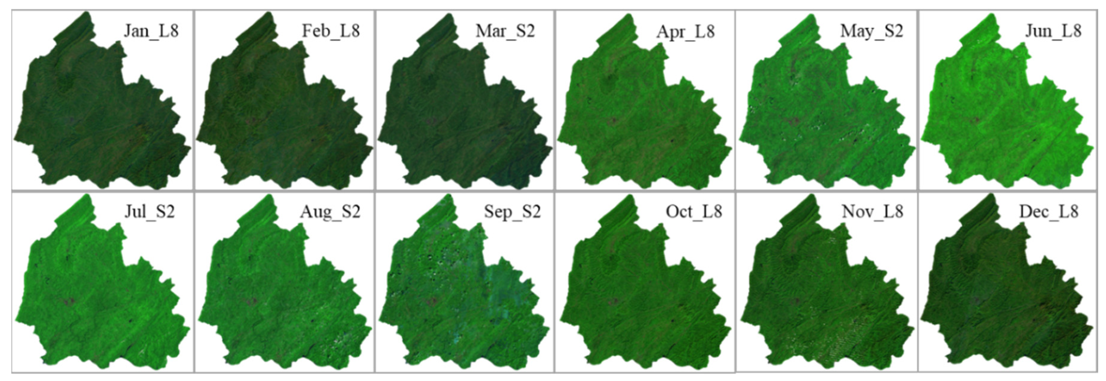
  • Image composition. The method described by [43] was used to composite a new image, which includes topographic corrections and image composition. The images from the same month were used to composite an image to obtain time-series images for the study area. Sentinel-2 data were used, and if for a specific month (e.g., June), an image covering the study area using Sentinel-2 could not be obtained, Landsat-8 data from the same month between 2016 and 2018 were used to compose the image. To ensure the consistency in spatial resolution for Landsat-8 and Sentinel-2, the all bands used for Landsat-8 were resampled to the same spatial resolution to Sentinel-2 (10 m). Finally, 12 images with only visible blue, green, red, and near-infrared bands for the study area with 10 m spatial resolution were generated, as shown in Figure 3.
  • NDVI time series creation. The NDVI was used to extract temporal patterns. This index is regarded as an appropriate spectral indicator of vegetation activity and phenological characteristics and a powerful and phenology-based method to carry out vegetation-cover classification at regional and global scales [29,44,45,46]. The NDVI has been generated from the red and near-infrared bands:
    NDVI = ρ N I R ρ R E D ρ N I R + ρ R E D

2.3.2. Classification

TWDTW was used to extract forest types, and two MLAs for classification—RF and SVM—were employed as comparisons with the results of the TWDTW algorithm.
1. Time-Weighted Dynamic Time Warping
TWDTW is based on the DTW method, which was originally proposed for speech recognition [37]. DTW is flexible to handle irregular sampling and out-of-phase time series and has achieved significant results in time-series analyses [47,48,49,50]. DTW works by comparing the similarity between temporal sequences and finds their optimal alignment, resulting in a dissimilarity measure [37,47]. For remote sensing, DTW can handle temporal distortions and compare shifted evolution profiles and irregular sampling because of its ability to align radiometric profiles optimally [51]. However, DTW disregards the temporal range when finding the best alignment between two time series [40]. TWDTW was developed by adding a time constraint to DTW to classify various land-cover types and has significantly improved the accuracy of DTW. The TWDTW method was implemented in the R (v3.4.4) package dtwSat v0.2.5 (São José dos Campos, Brazil) [40,52].
The classification process consists of two main steps:
Temporal pattern extraction. The temporal patterns of forest type had been extracted by using the pixel-based stack of NDVI datasets obtained from the time-series images and training samples. The function dtwSat::createPatterns [52] in the package was used to define the temporal patterns, which can create a smooth temporal pattern of the NDVI using the Generalized Additive Model (GAM) method [53]. The sampling frequency of the output patterns was set to 5 days.
Time-series image classification. A logistic TWDTW was implemented based on the R package “dtwSat” [52], which has a low penalty for small time warps and significant costs for large time warps [40,51]. Time warps are the inconsistency between the NDVI temporal pattern of the forest types to be classified and the created NDVI temporal pattern [40]. The two key parameters α and β were set to −0.1 and 50, as recommended in [40,51], thereby adding a time-weighted feature to the DTW, with a low penalty for time warps smaller than 50 days and a higher penalty for larger time warps.
2. Random Forest
RF is an integrated learning method based on a decision tree, which is combined with many ensemble regression or classification trees [54,55]. Its superiority is embodied in its relatively fast training speed, and the performance optimization process improves the accuracy of the RF model [56]. In the current study, RF had been implemented based on the scikit-learn package, which is an open-access data source and provides efficient machine learning tools in Python for data mining and data analysis [57]. Two parameters were tuned for RF, namely the number of trees which would be created by randomly selecting samples from the training samples (ntree parameter), and the number of variables used for tree node splitting (mtry parameter). In all three study areas, the ntree parameter was set to 1000 because previous studies had established that there is no increase in the number of errors beyond the creation of 1000 classification trees from randomly selected samples [58]. Following the RF classification results reported in previous studies and reviewed in Belgiu and Drăguţ [54] and Gislason et al. [59], the mtry parameter was established as the square root of the number of the available layers. Only the NDVI values computed from the time-series images and blue, green, red and near-infrared bands were used as input variables in the RF classifier.
3. Support Vector Machine
SVM is a traditional and advanced statistical MLA that separates the classes by an optimal decision hyperplane surface and obtains acceptable accuracy when classifying the remote-sensing images [60]. SVM had been also implemented using scikit-learn package in Python, and it has three parameters impacting the classification results, which are the kernel function (K), cost parameter (C), and gamma parameter (G). For the K, a radial bias function (RBF) yielded high performance with respect to convergence speed, robustness, and fewer parameter values to predefine [61]. The C tells the SVM optimization how much to avoid misclassifying each training example. The G defines the influence of a single training example. These two parameters were tuned with C = [10, 20, 30, 40, 50, 60, 70, 80, 90, 100] and G = [0.005, 0.01, 0.025, 0.05, 0.075, 0.1, 0.2, 0.3, 0.4, 0.5]. Finally, the RBF and the adjusted parameters of C factor = 70 and G = 0.2 were used in this study because these parameters provide the best results and high classification accuracy. The input variables in the SVM classifier are the same as RF classifier.

2.3.3. Comparison and Evaluation

The forest-type maps obtained by TWDTW, RF, and SVM were compared for spatial distribution and the area statistics of forest types. Then, these maps were evaluated for overall accuracy (OA) [62], producer accuracy, user accuracy metrics, and kappa coefficient (KC) [63] using the validation data available in Table 1.

3. Results

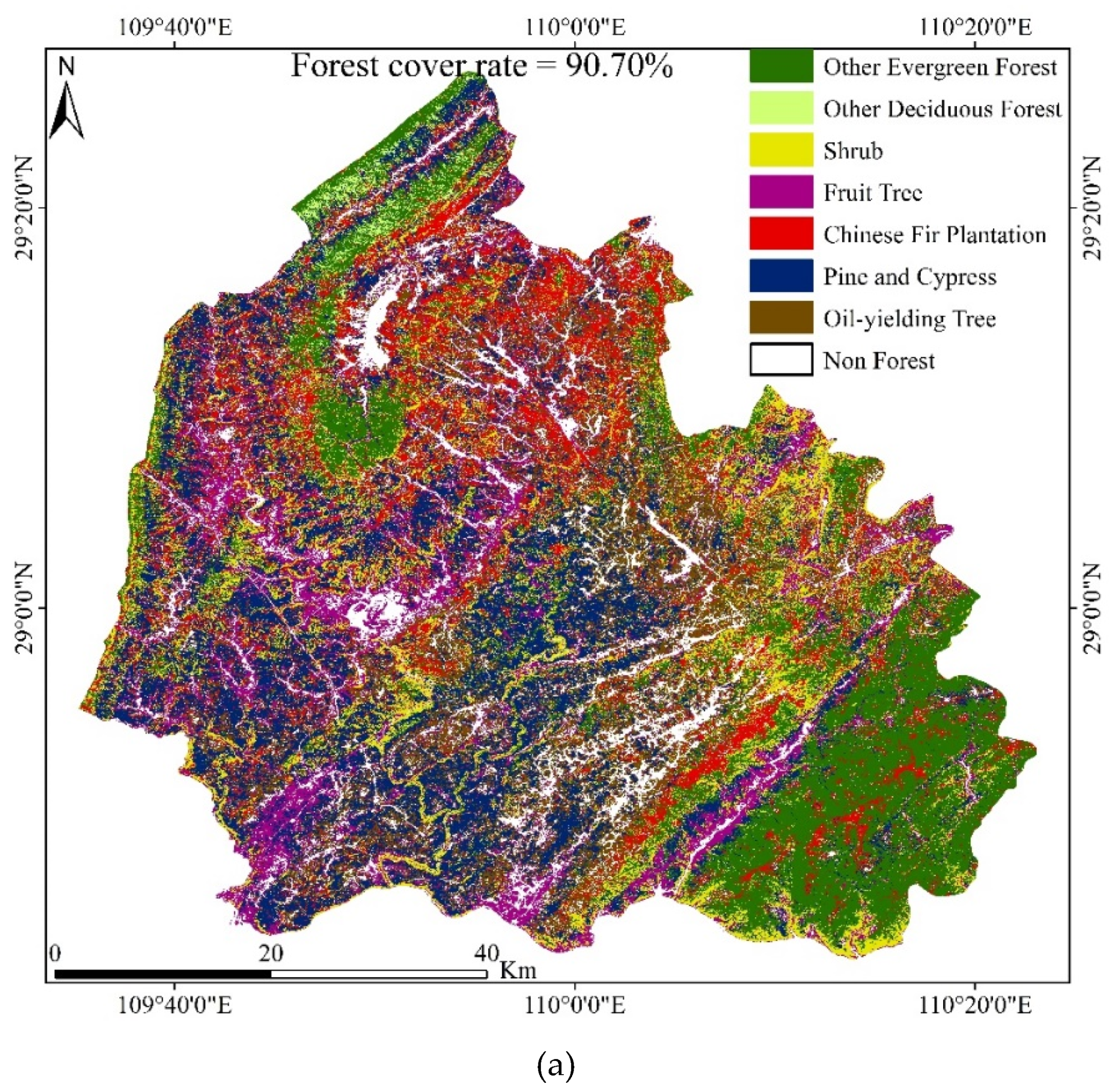
3.1. Classification Results

The forest-type maps obtained by TWDTW, RF, and SVM methods are presented in Figure 4a–c. The forest-type area ratios were calculated and are shown in Figure 5. The spatial distributions of forest types obtained by TWDTW, SVM, and RF are highly consistent. The spatial distributions of fruit trees (FT), oil-yielding trees (OYT), pine and cypress trees (PC) and shrubs (SHR), other evergreen forests (OEF), and other deciduous forests (ODF) are primarily concentrated in the southwest, northeast, middle, southeast, and northwest, respectively. TWDTW produced more CFP types, which are primarily distributed in the north, while the maps of RF and SVM show a smaller amount of CFPs, which are predominantly distributed in the southeast.
Figure 5 illustrates the details of the forest types, which indicates that TWDTW produced the largest area of forest (90.70%), followed by RF (90.47%) and SVM (90.23%). TWDTW produced larger areas of OEF and CFP compared with RF and SVM, while RF produced the largest area for ODF, SHR, FT, and OYT. The PC area of SVM was the most substantial of the three methods. In addition, PC comprised the largest portion of the research area, covering more than 20% of the total area, as determined by all three methods, while the area of FT was the smallest. CFP has the maximum difference determined by the three methods, among which TWDTW produced the largest area of CFP, while SVM has the smallest area of CFP. The differences in the other types of areas are not significant.

3.2. Evaluation

The TWDTW, RF, and SVM algorithms ran 10 times, and the mean overall accuracy (MOA) and mean kappa coefficient (MKC) are presented in Table 2. Compared with RF and SVM, TWDTW achieved the best results with MOA and MKC of 93.81% and 0.93, respectively, followed by RF with MOA and MKC of 91.54% and 0.90, while SVM produced the lowest values of MOA (89.66%) and MKC (0.88).
Table 2 also shows the variability in the TWDTW, RF, and SVM methods after 10 cycles. The OA and KC of the TWDTW method exhibit a much smaller range of variability than the RF and SVM methods, which are (±)0.003 and (±)0.002 respectively. In addition, RF achieved better classification accuracy than SVM, but with the biggest range of variability.
Figure 6 presents the mean producer accuracy (MPA) and mean user accuracy (MUA) for TWDTW, RF, and SVM methods after each had been run 10 times. TWDTW produced the highest MPA for FT (94.81%), ODF (96.49%), and OYT (96.61%), compared with the RF and SVM methods. RF produced the best MPA for OEF (86.67%) and SHR (94.59%) of the three methods. SVM only generated a better MPA for CFP (92.06%) compared with the other two methods. For MUA, TWDTW performed substantially better than RF and SVM in OEF, CFP, and OYT, especially for OEF and OYT, whose MUAs reached 100%. RF produced the highest MUA for SHR (87.50%) and ODF (93.33%), while SVM had not generated obvious advantages for any of the forest types.

4. Discussion

4.1. Identification of Temporal Patterns

The NDVI time series data were used to identify temporal patterns for the forest types because it was found to be sufficiently stable in permitting meaningful comparisons for seasonal and inter-annual changes in vegetation growth and activity [64]. The various forest types available present distinct temporal patterns (Figure 7), which reflect the unique growth trajectories of the forest types and provide evidence for forest-type classification. OEF has its period of maximum growth in April through December, and the NDVI began to decrease in December and reached the lowest value in February. FT reached its period of maximum growth from June until late September and began to decline near the end of September. SHR has two periods of maximum growth. The first is between April and July, and the other is between October and November, which is distinct from other forest types. This is probably because that SHR is one of the most abundant resources and has various species [65]. ODF began growth in March and has the highest values of NDVI from June through September. CFP reached its peak growing period NDVI in July and lasted until early December. PC displayed a similar trend to OEF, but the overall values of NDVI are much smaller than those of OEF. OYT reached the peak of NDVI in June, and the growing period lasted through early November.
In previous studies, the NDVI time series data were applied successfully to temporal pattern identification and classification of cropland. For example, Yan et al. [66] used the NDVI time series derived from Landsat-8 images to determine the growth patterns of cropland and achieved automatic cropland classifications using this pattern. Belgiu and Csillik [51] recently calculated the NDVI time series of Sentinel-2, applied them to three different study areas, and performed temporal pattern identification and classification of cropland. Therefore, this index was selected to study the temporal pattern of forest types because forests are similar to cropland in that they both have seasonal change characteristics. However, other vegetation indices have also been widely used and have achieved satisfactory results for temporal pattern recognition of vegetation. For example, Manabe et al. [67] studied the temporal patterns of cropland using EVI time-series data and achieved classification based on the TWDTW method. Viana et al. [68] combined NDVI and normalized difference water index (NDWI) and used them to identify the characteristics of land-cover types and developed land cover maps. Because all vegetation indices could not be explored at this time, the current study was limited to the NDVI. The results also demonstrated that the NDVI time series could reflect the growth characteristics of the various forest types, and combined with the TWDTW algorithm, can attain the classification of complex mountain forest types. It’s worth noting that we used two products with different correction-level to construct the NDVI time series, which exists impact on identification of true NDVI value. However, this will not affect the consistency of the time series pattern of NDVI. some previous studies also mentioned that the atmospheric correction could not improve the classification accuracy [69,70]. Therefore, this inconsistency of original data will not influence our classification results. In addition, this study discussed the phenology pattern for each category, but, did not carry out phenological pattern analysis at tree species level, which mainly due to the lack of detail data for tree species. However, the method used in this study could provide reference for tree species identification supported by the necessary tree species sample data.

4.2. Comparison of TWDTW, RF, and SMV Methods

The MPA and MUA in Figure 6 show the performance of TDWTW, RF, and SVM for the discrimination of different forest types. TWDTW produced higher MPA and MUA for OYT (see Figure 6), while it produced lower MPA and MUA for SHR and OEF, which may be attributed to the high intra-class spectral heterogeneity. In addition, RF acquired the second-best results and produced the highest MPA and MPA for SHR. This result confirms the efficiency of the RF classifier for forest-type mapping that had been reported in previous studies [33,71,72]. For the forest distribution of the three maps (Figure 4), there is no significant difference overall, which establishes the effectiveness of all three methods. However, there are some differences in the total area of the specific forest types among the three methods. Compared with the other two methods, the total area of forest obtained by the TWDTW algorithm is the largest. The most apparent difference is in the extraction of the Chinese fir plantation (Figure 8). The TWDTW algorithm noticeably acquired more area, as shown in Figure 8, followed by RF and SVM. Additionally, the evaluation results have specified that the MPA and MUA of CFP were the highest, which indicates that the TWDTW algorithm can substantially capture more variations in the growth patterns of the distinct types of forest and better differentiate the various forest types in the case of limited training data.
All results have suggested that the TWDTW method is more suitable for forest-type classification in mountainous areas. However, various mountainous areas may provide different results. Therefore, another experiment was conducted for a different mountainous area. The obtained classification and accuracy evaluation results are shown in Figure 9 and Table 3. Compared with the RF and SVM methods, TWDTW still obtained the highest overall accuracy (93.44%) and kappa coefficient (0.92), which is in accordance with the results of this study and demonstrates the robustness of the TWDTW algorithm in mountain forest-type classifications.

4.3. Sensitivity to the Number of Training Data

Three additional analyses were conducted to verify that TWDTW can produce more stable results than RF and SVM with fewer training samples. Each experiment selected 1/2, 1/3, and 1/4 of the training data from each category in Table 1 to rebuild the training set and used the validation data in Table 1 for validation and evaluation. The evaluation results are shown in Figure 10. TWDTW produced the highest overall accuracies and kappa coefficients with a small number of training samples. As the number of training data gradually decreased, the accuracy of the three methods also declined. However, the accuracy of the TWDTW algorithm remained the highest, and its variability was smaller than that of the RF and SVM algorithms. Previous studies have also reported that TWDTW has generated classification results with higher accuracy for small training samples [55]. For RF and SVM, the overall accuracies and kappa coefficients of the classification results were lower than those of TWDTW. This is consistent with previous studies that MLAs have achieved less accurate results when a small number of training samples is applied [51,73,74]. These findings provide evidence to use the TWDTW method to classify forest types, especially for mountainous areas where abundant training samples cannot be acquired. In addition, Petitjean et al. [50] reported that TWDTW also has the advantage of being robust with irregular temporal sampling and the annual changes in vegetation phenological cycles. This makes TWDTW flexible and valuable for forest-type classifications, especially in regions with high meteorological variability.

4.4. Combination of Sentinel-2 and Landsat-8 Time Series

In addition to the application of the TWDTW algorithm, this research benefits from the combined application of the Sentinel-2 and Landsat-8 time-series data. Because the study area is located in a mountainous area where the altitude is high, the summer is hot and rainy, and there is often cloud cover, it is difficult to obtain high-quality remote sensing images in the peak season of vegetation growth. We tried to only use Sentinel-2 data, but we found that it was impossible to obtain high-quality time-series remote sensing data for the entire research area. Therefore, the two types of data (Sentinel-2 and Landsat-8) were combined, and the time-series NDVI data were obtained that reflect the temporal characteristics of the study area. This combination is one of the critical foundations for the success of this study.
The potential of time-series data has been evaluated for forest-type classifications in various studies [22,23,24,25]. However, the application of Sentinel-2 and Landsat-8 time-series images for forest-type classification in a mountainous area had not been reported. Therefore, this study provides a valid case study using the Sentinel-2 and Landsat-8 time-series images for forest-type classifications in a mountainous area. However, some limitations still exist. This study was limited to the utilization of blue, green, red, and near-infrared bands and the NDVI index in the classification procedures. In future studies, red edge bands from Sentinel-2 sensors, which are sensitive to vegetation, and other indices such as enhanced vegetation index (EVI) and normalized difference water index (NDWI) could be considered for forest-type mapping. Additionally, synthetic aperture radar (SAR) data can reduce the cloud occlusions problem [75,76], which may be combined with multi-spectral images to improve the classification of forest types.

5. Conclusions

In this study, Sentinel-2 and Landsat-8 time-series data were used as input data to evaluate the effects of TWDTW and MLAs—RF and SVM—on forest-type classification in complex mountainous areas. A mountainous area in southern China was evaluated and analyzed regarding spatial distribution and accuracy evaluation. Forest-type maps obtained by TWDTW, RF, and SVM presented highly consistent spatial distribution. However, TWDTW outperformed SVM and RF in the quality of the classification output, as measured by the overall accuracy, kappa coefficient, producer accuracy, and user accuracy. It was also demonstrated that TWDTW was more robust than the RF and SVM methods regarding the amount of training data. These results have established that TWDTW could be used to map forest types for mountainous areas accurately using time-series data.

Author Contributions

K.C. drafted the manuscript and was responsible for data preparation, experimentation, and analysis. J.W. was responsible for the research program design and results analysis, and reviewed the manuscript.

Funding

This research was funded by “Strategic Priority Research Program (class A) of the Chinese Academy of Sciences, grant number XDA19040501”, “The 13th Five- year Informatization Plan of the Chinese Academy of Sciences, grant number XXH13505- 07”, and “Construction Project of China Knowledge Center for Engineering Sciences and Technology, grant number CKCEST-2019-3-6”.

Conflicts of Interest

The authors declare no conflict of interest.

References

  1. Tang, S.Q. Soil and water conservation of forest in mountain area. Fujian Soil Water Conserv. 2003, 2, 10–13. [Google Scholar]
  2. Iverson, L.R.; Graham, R.L.; Cook, E.A. Applications of satellite remote sensing to forested ecosystems. Landsc. Ecol. 1989, 3, 131–143. [Google Scholar] [CrossRef]
  3. Kerr, J.T.; Ostrovsky, M. From space to species: Ecological applications for remote sensing. Trends Ecol. Evol. 2003, 18, 299–305. [Google Scholar] [CrossRef]
  4. Liu, Y.; Gong, W.; Hu, X.; Gong, J. Forest Type Identification with Random Forest Using Sentinel-1A, Sentinel-2A, Multi-Temporal Landsat-8 and DEM Data. Remote Sens. 2018, 10, 946. [Google Scholar] [CrossRef]
  5. Lei, G.B.; Li, A.N.; Bian, J.H.; Zhang, Z.J.; Zhang, W.; Wu, B.F. An practical method for automatically identifying the evergreen and deciduous characteristic of forests at mountainous areas: A case study in Mt.Gongga Region. Acta Ecol. Sin. 2014. [Google Scholar] [CrossRef]
  6. Peterson, D.L.; Spanner, M.A.; Running, S.W.; Teuber, K.B. Relationship of thematic mapper simulator data to leaf area index of temperate coniferous forest. Remote Sens. Environ. 1987, 22, 323–341. [Google Scholar] [CrossRef]
  7. Ardö, J. Volume quantification of coniferous forest compartments using spectral radiance recorded by Landsat Thematic Mapper. Int. J. Remote Sens. 1992, 13, 1779–1786. [Google Scholar] [CrossRef]
  8. Congalton, R.G.; Green, K.; Teply, J. Mapping old growth forests on national forest and park lands in the Pacific Northwest from remotely sensed data. Photogramm. Eng. Remote Sens. 1993, 59, 529–535. [Google Scholar]
  9. Gemmell, F.M. Effects of forest cover, terrain, and scale on timber volume estimation with thematic mapper data in a rocky mountain site. Remote Sens. Environ. 1995, 51, 291–305. [Google Scholar] [CrossRef]
  10. Martin, M.E.; Newman, S.D.; Aber, J.D.; Congalton, R.G. Determining forest species using high spectral resolution remote sensing data. Remote Sens. Environ. 1998, 65, 249–254. [Google Scholar] [CrossRef]
  11. Kilpeläinen, P.; Tokola, T. Gain to be achieved from stand delineation in LANDSAT TM image-based estimates of stand volume. For. Ecol. Manag. 1999, 124, 105–111. [Google Scholar] [CrossRef]
  12. Pax-Lenney, M.; Woodcock, C.E.; Macomber, S.A.; Song, C. Forest mapping with a generalized classifier and Landsat TM data. Remote Sens. Environ. 2001, 77, 241–250. [Google Scholar] [CrossRef]
  13. Tokola, T.; Sarkeala, J.; Linden, M.V.D. Use of topographic correction in Landsat TM-based forest interpretation in Nepal. Int. J. Remote Sens. 2001, 22, 551–563. [Google Scholar] [CrossRef]
  14. Dorren, L.K.A.; Maier, B.; Seijmonsbergen, A.C. Improved Landsat-based forest mapping in steep mountainous terrain using object-based classification. For. Ecol. Manag. 2003, 183, 31–46. [Google Scholar] [CrossRef]
  15. Kosaka, N.; Akiyama, T.; Tsai, B.; Kojima, T. Forest type classification using data fusion of multispectral and panchromatic high-resolution satellite imageries. In Proceedings of the IGARSS ′05 2005 IEEE International Geoscience and Remote Sensing Symposium, Seoul, Korea, 29 July 2005. [Google Scholar]
  16. Ruefenacht, B.; Finco, M.V.; Nelson, M.D.; Czaplewski, R.; Helmer, E.H.; Blackard, J.A.; Holden, G.R.; Lister, A.J.; Salajanu, D.; Weyermann, D.; et al. Conterminous U.S. and Alaska Forest Type Mapping Using Forest Inventory and Analysis Data. Photogramm. Eng. Remote Sens. 2008, 74, 1379–1388. [Google Scholar] [CrossRef]
  17. Kim, M.; Madden, M.; Warner, T.A. Forest Type Mapping using Object-specific Texture Measures from Multispectral Ikonos Imagery. Photogramm. Eng. Remote Sens. 2009, 75, 819–829. [Google Scholar] [CrossRef]
  18. Kempeneers, P.; Sedano, F.; Seebach, L.; Strobl, P.; San-Miguel-Ayanz, J. Data Fusion of Different Spatial Resolution Remote Sensing Images Applied to Forest-Type Mapping. IEEE Trans. Geosci. Remote Sens. 2011, 49, 4977–4986. [Google Scholar] [CrossRef]
  19. Laurel, B.; Leonhard, B.; Ellen, H.; Kruse, B. Tree Species Classification Using Hyperspectral Imagery: A Comparison of Two Classifiers. Remote Sens. 2016, 8, 445. [Google Scholar]
  20. Zhang, X.; Treitz, P.M.; Chen, D.; Quan, C.; Shi, L.; Li, X. Mapping mangrove forests using multi-tidal remotely-sensed data and a decision-tree-based procedure. Int. J. Appl. Earth Obs. Geoinf. 2017, 62, 201–214. [Google Scholar] [CrossRef]
  21. Jia, M.M.; Ren, C.Y.; Liu, D.W.; Wang, Z.M.; Tang, X.G.; Dong, Z.Y. Object-oriented forest classification based on combination of HJ-1 CCD and MODISNDVI data. Acta Ecol. Sin. 2014, 34, 7167–7174. [Google Scholar]
  22. Grabska, E.; Hostert, P.; Pflugmacher, D.; Ostapowicz, K. Forest Stand Species Mapping Using the Sentinel-2 Time Series. Remote Sens. 2019, 11, 1197. [Google Scholar] [CrossRef]
  23. Pasquarella, V.J.; Holden, C.E.; Woodcock, C.E. Improved mapping of forest type using spectral-temporal Landsat features. Remote Sens. Environ. 2018, 210, 193–207. [Google Scholar] [CrossRef]
  24. Zhu, X.; Liu, D. Accurate mapping of forest types using dense seasonal Landsat time-series. ISPRS J. Photogramm. Remote Sens. 2014, 96, 1–11. [Google Scholar] [CrossRef]
  25. Cheng, K.; Wang, J. Forest Type Classification Based on Integrated Spectral-Spatial-Temporal Features and Random Forest Algorithm—A Case Study in the Qinling Mountains. Forests 2019, 10, 559. [Google Scholar] [CrossRef]
  26. Li, M.; Im, J.; Beier, C. Machine learning approaches for forest classification and change analysis using multi-temporal Landsat TM images over Huntington Wildlife Forest. GISci. Remote Sens. 2013, 50, 361–384. [Google Scholar] [CrossRef]
  27. Duro, D.C.; Franklin, S.E.; Dubé, M.G. A comparison of pixel-based and object-based image analysis with selected machine learning algorithms for the classification of agricultural landscapes using SPOT-5 HRG imagery. Remote Sens. Environ. 2012, 118, 259–272. [Google Scholar] [CrossRef]
  28. Lu, D.; Weng, Q. A survey of image classification methods and techniques for improving classification performance. Int. J. Remote Sens. 2007, 28, 823–870. [Google Scholar] [CrossRef]
  29. Potapov, P.V.; Dempewolf, J.; Talero, Y.; Hansen, M.C.; Stehman, S.V.; Vargas, C.; Rojas, E.J.; Castillo, D.; Mendoza, E.; Calderón, A.; et al. National satellite-based humid tropical forest change assessment in Peru in support of REDD+ implementation. Environ. Res. Lett. 2014, 9, 124012. [Google Scholar] [CrossRef]
  30. Bader, M.Y.; Ruijten, J.J.A. A topography-based model of forest cover at the alpine tree line in the tropical Andes. J. Biogeogr. 2008, 35, 711–723. [Google Scholar] [CrossRef]
  31. Gottlicher, D.; Obregon, A.; Homeier, J.; Rollenbeck, R.; Nauss, T.; Bendix, J. Land-cover Classification in the Andes of Southern Ecuador Using Landsat ETM+ Data as a Basis for SVAT Modelling. Int. J. Remote Sens. 2009, 30, 1867–1886. [Google Scholar] [CrossRef]
  32. Gudex-Cross, D.; Pontius, J.; Adams, A. Enhanced forest cover mapping using spectral unmixing and object-based classification of multi-temporal Landsat imagery. Remote Sens. Environ. 2017, 196, 193–204. [Google Scholar] [CrossRef]
  33. Luis, V.I.; Yasumasa, H.; Lenin, V.S.; Noemi, S.T. Natural Forest Mapping in the Andes (Peru): A Comparison of the Performance of Machine-Learning Algorithms. Remote Sens. 2018, 10, 782. [Google Scholar]
  34. Wessel, M.; Brandmeier, M.; Tiede, D. Evaluation of Different Machine Learning Algorithms for Scalable Classification of Tree Types and Tree Species Based on Sentinel-2 Data. Remote Sens. 2018, 10, 1419. [Google Scholar] [CrossRef]
  35. Rodriguez-Galiano, V.F.; Ghimire, B.; Rogan, J.; Chica-Olmo, M.; Rigol-Sanchez, J.P. An assessment of the effectiveness of a random forest classifier for land-cover classification. ISPRS J. Photogramm. Remote Sens. 2012, 67, 93–104. [Google Scholar] [CrossRef]
  36. Nitze, I.; Schulthess, U.; Asche, H. Comparison of machine learning algorithms random forest, artificial neural network and support vector machine to maximum likelihood for supervised crop type classification. In Proceedings of the 4th GEOBIA, Rio de Janeiro, Brazil, 7–9 May 2012; pp. 7–9. [Google Scholar]
  37. Sakoe, H.; Chiba, S. Dynamic programming algorithm optimization for spoken word recognition. IEEE Trans. Acoust. Speech Signal Process. 1978, 26, 43–49. [Google Scholar] [CrossRef]
  38. Baumann, M.; Ozdogan, M.; Richardson, A.D.; Radeloff, V.C. Phenology from Landsat when data is scarce: Using MODIS and dynamic time-warping to combine multi-year Landsat imagery to derive annual phenology curves. Int. J. Appl. Earth Obs. Geoinf. 2017, 54, 72–83. [Google Scholar] [CrossRef]
  39. Petitjean, F.; Inglada, J.; Gançarski, P. Satellite image time series analysis under time warping. IEEE Trans. Geosci. Remote Sens. 2012, 50, 3081–3095. [Google Scholar] [CrossRef]
  40. Maus, V.; Camara, G.; Cartaxo, R.; Sanchez, A.; Ramos, F.M.; Queiroz, G.R.D. A time-weighted dynamic time warping method for land-use and land-cover mapping. IEEE J. Sel. Top. Appl. Earth Obs. Remote Sens. 2016, 9, 1–11. [Google Scholar] [CrossRef]
  41. Chen, Z. Feature and administering studying of the landslide at center street, Huitong county. Hunan Geol. 1999, 18, 249–260. [Google Scholar]
  42. Segovia, A.R.; Bullock, E.L.; Corral, L.; Nolte, C. Project Impact Assessment on Deforestation and Forest Degradation (1-44, Rep. No. 2149/BL-GU). Available online: https://hdl.handle.net/2144/31321 (accessed on 31 August 2019).
  43. Hurni, K.; Heinimann, A.; Würsch, L. Technical Report. Centre for Development and Environment (CDE) University of Bern, (Google Earth Engine Image Pre-processing Tool: Background and Methods). 2017. Available online: https://www.cde.unibe.ch/e65013/e542846/e707304/e707386/e707388/CDE_Pre-processingTool-BackgroundAndMethods_eng.pdf (accessed on 9 October 2019).
  44. Potapov, P.; Turubanova, S.; Hansen, M.C. Regional-scale boreal forest cover and change mapping using Landsat data composites for European Russia. Remote Sens. Environ. 2011, 115, 548–561. [Google Scholar] [CrossRef]
  45. Wardlow, B.D.; Egbert, S.L.; Kastens, J.H. Analysis of Time-Series MODIS 250m Vegetation Index Data for Crop Classification in the US Central Great Plains. Remote Sens. Environ. 2007, 108, 290–310. [Google Scholar] [CrossRef] [Green Version]
  46. Jia, M.; Wang, Z.; Wang, C.; Mao, D.; Zhang, Y. A New Vegetation Index to Detect Periodically Submerged Mangrove Forest Using Single-Tide Sentinel-2 Imagery. Remote Sens. 2019, 11, 2043. [Google Scholar] [CrossRef] [Green Version]
  47. Lawrence, R.; Juang, B. Fundamentals of Speech Recognition; Prentice-Hall International, Inc.: Upper Saddle River, NJ, USA, 1993. [Google Scholar]
  48. Berndt, D.J.; Clifford, J. Using Dynamic Time Warping to Find Patterns in Time Series. In KDD Workshop; Fayyad, U.M., Uthurusamy, R., Eds.; AAAI Press: Seattle, WA, USA, 1994; pp. 359–370. [Google Scholar]
  49. Eamonn, K.; Ratanamahatana, C.A. Exact Indexing of Dynamic Time Warping. Knowl. Inf. Syst. 2005, 7, 358–386. [Google Scholar]
  50. Petitjean, F.; Weber, J. Efficient satellite image time series analysis under time warping. IEEE Geosci. Remote Sens. Lett. 2014, 11, 1143–1147. [Google Scholar] [CrossRef]
  51. Belgiu, M.; Csillik, O. Sentinel-2 cropland mapping using pixel-based and object-based time-weighted dynamic time warping analysis. Remote Sens. Environ. 2017, 204, 509–523. [Google Scholar] [CrossRef]
  52. Victor, M.; Gilberto, C.; Marius, A.; Pebesma, E. Dtwsat: Time-Weighted Dynamic Time Warping for Satellite Image Time Series Analysis in R. J. Stat. Softw. 2019, 88, 1–31. [Google Scholar] [CrossRef] [Green Version]
  53. Wood, S.N. Fast stable restricted maximum likelihood and marginal likelihood estimation of semiparametric generalized linear models. J. R. Stat. Soc. Ser. B Stat. Methodol. 2011, 73, 3–36. [Google Scholar] [CrossRef] [Green Version]
  54. Belgiu, M.; Drăguţ, L. Random forest in remote sensing: A review of applications and future directions. ISPRS J. Photogramm. Remote Sens. 2016, 114, 24–31. [Google Scholar] [CrossRef]
  55. Breiman, L. Random forest. Mach. Learn. 2001, 45, 5–32. [Google Scholar] [CrossRef] [Green Version]
  56. Liaw, A.; Wiener, M. Classification and regression by random Forest. R News 2002, 2, 18–22. [Google Scholar]
  57. Pedregosa, F.; Varoquaux, G.; Gramfort, A.; Michel, V.; Thirion, B.; Grisel, O.; Blondel, M.; Prettenhofer, P.; Weiss, R.; Dubourg, V.; et al. Scikit-learn: Machine learning in Python. J. Mach. Learn. Res. 2011, 12, 2825–2830. [Google Scholar]
  58. Lawrence, R.L.; Wood, S.D.; Sheley, R.L. Mapping invasive plants using hyperspectral imagery and Breiman cutler classifications (Random Forest). Remote Sens. Environ. 2006, 100, 356–362. [Google Scholar] [CrossRef]
  59. Gislason, P.O.; Benediktsson, J.A.; Sveinsson, J.R. Random forests for land cover classification. Pattern Recogn. Lett. 2006, 27, 294–300. [Google Scholar] [CrossRef]
  60. Hasan, S.; Shi, W.; Zhu, X.; Abbas, S. Monitoring of Land Use/Land Cover and Socioeconomic Changes in South China over the Last Three Decades Using Landsat and Nighttime Light Data. Remote Sens. 2019, 11, 1658. [Google Scholar] [CrossRef] [Green Version]
  61. Huang, C.; Song, K.; Kim, S.; Townshend, J.R.G.; Davis, P.; Masek, J.G.; Goward, S.N. Use of a dark object concept and support vector machines to automate forest cover change analysis. Remote Sens. Environ. 2008, 112, 970–985. [Google Scholar] [CrossRef]
  62. Congalton, R.G. A review of assessing the accuracy of classifications of remotely sensed data. Remote Sens. Environ. 1991, 37, 35–46. [Google Scholar] [CrossRef]
  63. Cohen, J. A coefficient of agreement for nominal scales. Educ. Psychol. Meas. 1960, 20, 37–46. [Google Scholar] [CrossRef]
  64. Huete, A.; Didan, K.; Miura, T.; Rodriguez, E.P.; Gao, X.; Ferreira, L.G. Overview of the radiometric and biophysical performance of the MODIS vegetation indices. Remote Sens. Environ. 2002, 83, 195–213. [Google Scholar] [CrossRef]
  65. Ma, Y.Z. Study on application of bushes and shrubs in planting landscape of Hunan. Hunan For. Sci. Technol. 2006, 1, 49–51. [Google Scholar]
  66. Yan, L.; Roy, D.P. Automated crop field extraction from multi-temporal web enabled Landsat data. Remote Sens. Environ. 2014, 144, 42–64. [Google Scholar] [CrossRef] [Green Version]
  67. Manabe, V.D.; Melo, M.R.S.; Rocha, J.V. Framework for Mapping Integrated Crop-Livestock Systems in Mato Grosso, Brazil. Remote Sens. 2018, 10, 1322. [Google Scholar] [CrossRef] [Green Version]
  68. Viana, C.M.; Girão, I.; Rocha, J. Long-Term Satellite Image Time-Series for Land Use/Land Cover Change Detection Using Refined Open Source Data in a Rural Region. Remote Sens. 2019, 11, 1104. [Google Scholar] [CrossRef] [Green Version]
  69. Chinsu, L.; Wu, C.C.; Tsogt, K.; Ouyang, Y.C.; Chang, C.I. Effects of Atmospheric Correction and Pansharpening on LULC Classification Accuracy Using WorldView-2 Imagery. Inf. Process. Agric. 2015, 2, 25–36. [Google Scholar]
  70. Song, C.; Woodcock, C.; Seto, K.; Lenney, M.P.; Macomber, S. Classification and Change Detection Using Landsat TM Data: When and How to Correct Atmospheric Effects? Remote Sens. Environ. 2001, 75, 230–244. [Google Scholar] [CrossRef]
  71. Hao, P.; Zhan, Y.; Wang, L.; Niu, Z.; Shakir, M. Feature selection of time series MODIS data for early crop classification using random forest: A case study in Kansas, USA. Remote Sens. 2015, 7, 5347–5369. [Google Scholar] [CrossRef] [Green Version]
  72. Pelletier, C.; Valero, S.; Inglada, J.; Champion, N.; Dedieu, G. Assessing the robustness of random forests to map land cover with high resolution satellite image time series over large areas. Remote Sens. Environ. 2016, 187, 156–168. [Google Scholar] [CrossRef]
  73. Millard, K.; Richardson, M. On the importance of training data sample selection in random forest image classification: A case study in peatland ecosystem mapping. Remote Sens. 2015, 7, 8489–8515. [Google Scholar] [CrossRef] [Green Version]
  74. Valero, S.; Morin, D.; Inglada, J.; Sepulcre, G.; Arias, M.; Hagolle, O.; Dedieu, G.; Bontemps, S.; Defourny, P.; Koetz, B. Production of a dynamic cropland mask by processing remote sensing image series at high temporal and spatial resolutions. Remote Sens. 2016, 8, 55. [Google Scholar] [CrossRef] [Green Version]
  75. Reiche, J.; Hamunyela, E.; Verbesselt, J.; Hoekman, D.; Herold, M. Improving near-real time deforestation monitoring in tropical dry forests by combining dense Sentinel-1 time series with Landsat and ALOS-2 PALSAR-2. Remote Sens. Environ. 2018, 2018, 147–161. [Google Scholar] [CrossRef]
  76. Mizuochi, H.; Hayashi, M.; Tadono, T. Development of an Operational Algorithm for Automated Deforestation Mapping via the Bayesian Integration of Long-Term Optical and Microwave Satellite Data. Remote Sens. 2019, 11, 2038. [Google Scholar] [CrossRef] [Green Version]
Figure 1. Location of study area in China. The image to the left is a true color composite (red, green, blue bands) from Sentinel-2.
Forests 10 01040 g001
Figure 2. The workflow of TWDTW, RF, and SVM methods for forest type classification.
Forests 10 01040 g002
Figure 3. The input time-series images.
Forests 10 01040 g003
Figure 4. Forest type classification results obtained using TWDTW (a), RF (b), and SVM (c) methods.
Forests 10 01040 g004aForests 10 01040 g004b
Figure 5. Area ratio (%) of forest types, where OEF represents other evergreen forests, ODF represents other deciduous forests, SHR represents shrubs, FT represents fruit trees, CFP represent Chinese fir plantations, PC represents pine and cypress trees, and OYT represents oil-yielding trees.
Forests 10 01040 g005
Figure 6. Comparison of forest-type classification accuracy using TWDTW, RF, and SVM methods.
Forests 10 01040 g006
Figure 7. Temporal patterns of NDVI for all classes mapped, where OEF represents other evergreen forests, ODF represents other deciduous forests, SHR represents shrubs, FT represents fruit trees, CFP represent Chinese fir plantations, PC represents pine and cypress trees, and OYT represents oil-yielding trees.
Forests 10 01040 g007
Figure 8. Comparison of forest-type maps in detail acquired by TWDTW, RF, and SVM.
Forests 10 01040 g008
Figure 9. Classification maps obtained using TWDTW, RF, and SVM in another test area.
Forests 10 01040 g009
Figure 10. Overall accuracy (OA (%)) and kappa coefficient (KC) of TWDTW, SVM, and RF applied to the test area using 1/2, 1/3, and 1/4 of the training samples per class.
Forests 10 01040 g010
Table 1. Number of training and validation samples for each forest type
Forest TypeAbbreviationTrainingValidation
Other evergreen treesOEF6060
Other deciduous treesODF7171
ShrubSHR8080
Fruit treeFT7575
Chinese fir plantationCFP6767
Pine and cypressPC7373
Oil-yielding treeOYT5757
Non-forestNon5050
Table 2. Mean overall accuracy (MOA) and mean kappa coefficient (MKC) of TWDTW, RF, and SVM applied to the test area.
MethodMOA (%)MKC
TWDTW93.81 (±0.003)0.93 (±0.002)
RF91.54 (±0.004)0.90 (±0.005)
SVM89.66 (±0.005)0.88 (±0.006)
Table 3. Overall accuracy (OA) and kappa coefficient of TWDTW, RF, and SVM applied to another test area.
MethodOA (%)KC
TWDTW93.440.92
RF91.110.89
SVM89.190.87

