Variation in Carbon Concentration and Allometric Equations for Estimating Tree Carbon Contents of 10 Broadleaf Species in Natural Forests in Northeast China

Abstract

In this study, the effects of tree species, tissue types, and tree size on the carbon concentration were studied, and the two additive systems, one with tree diameter (D), and the other with both D and tree height (H), were developed to estimate the stem, root, branch, and foliage carbon content of 10 broadleaf species in northeast China. The coefficients of the two systems were estimated with the nonlinear seemingly unrelated regression (NSUR), while the heteroscedasticity of the model residual was solved with the weight function. Our results showed that carbon concentrations varied along with tree species and size; the tissues and foliage contained higher carbon concentration than other observed tissues. The two additive carbon equation systems exhibited good predictive and fitting performance, with R_a² > 0.87, average prediction error of approximately 0, and small average absolute error and absolute error percentage. The carbon equation system constructed with D and H exhibited better fit and performance, particularly for the stem and total carbon. Thus, the additive carbon equation systems estimated the tree carbon of 10 broadleaf species more accurately. These carbon equations can be used to monitor the carbon pool sizes for natural forests in the Chinese National Forest Inventory.

1. Introduction

According to the reports from the Food and Agriculture Organization [1], forestry occupies approximately 31% of the earth’s land area, meaning it has an indispensable role in the global carbon cycle. Almost 33.3% of the atmospheric CO₂ concentration is reduced by forests, because of their carbon storage ability (approximately 2.4 Pg) and emission sequestration of CO₂ (approximately 30%) [2,3]. Nowadays, more studies are underlining non-timber forest ecosystem services, such as natural hazards and biodiversity protection, and air and water cleaning. Globally, temperate mixed forests are mainly located in northeastern Europe, North America, and eastern Asia. In Asia, the majority of the temperate forests are distributed in the northeastern part of China, particularly in Heilongjiang province, which is a vital province in the climatic system and national carbon budget in China [4,5].

Among the studies on global climate change and carbon cycles, the quantity, distribution, and dynamics of forest carbon stocks are the hotspots and also remain a high priority for the prediction of forest growth and yield [3,6,7]. The main essential task for successfully implementing the initiatives of Reducing Emissions from Deforestation and Forest Degradation (REDD+), as well as for the conservation and enhancement of forest carbon stocks and sustainable management of forests is the development of allometric models for carbon accounting across different tree species. By doing this, those developing countries can receive financial bonuses for decreased carbon emissions [8,9]. However, few literature studies have been conducted on predictive models for quantifying the total and tissue carbon of broadleaf species.

To date, indirect and direct methods have been used to estimate individual tree carbon [10]. For the indirect methods, the individual tree carbon is calculated by multiplying the carbon concentration by the tree biomass, where the biomass is estimated using biomass equations [11,12]. When estimating forest carbon, 50% or 45% is generally used as the average carbon concentration for all species and forest types at regional and national scales; however, some others have used other carbon concentrations [10,13]. In general, the commonly accepted carbon concentrations are 50% for woody tissues, or 45%–50% for nonwoody tissues [14,15]. However, more and more studies have shown that the commonly used 45% or 50% carbon concentrations lead to certain errors [16,17,18,19,20], because of the various carbon concentrations among forest regions, tissue types, species, and sizes of trees [10,16,21]. For the direct methods, the carbon allometric equations are constructed using data obtained from a carbon analyzer when burning trees [10,22,23]. In summary, carbon allometric equations are essential and necessary if accurate fluxes and carbon stocks of natural forests are required.

It is common to use the diameter at breast height (D) as the only reliable predictor of the total and tissue biomass or carbon in most cases [4,9,10,24,25]. The tree height (H), another variable of the tree, can also be used as a predictor [9,25,26]. Adding H into biomass or carbon equations as another predictor notably improves the model performance by explaining the divergences and avoiding the potential limitations [25,27,28,29]. Thus, the regression with D and H was more reliable for prediction of the carbon in a forest.

The estimating equations for the total and tissue carbon of trees are categorized as nonadditive or additive models. The nonadditive equations cannot suit the total and tissue carbon data synchronously, leading to unequal total tissue carbon derived from the tissue and the total carbon model. The additive carbon equations fit the total and tissue carbon data simultaneously, which explicates the instinctive correlations among carbon tissues of the same sample [25,27,28,29], where the sum of carbon predictions from the tissue carbon model and from the total carbon models are the same [30,31]. For the additive carbon equations, various parameter estimation methods and model specifications were used in linear and nonlinear models [30,31,32,33]. Among these, nonlinear seemingly unrelated regression (NSUR) and seemingly unrelated regression (SUR) are more widely used. An advantage of using SUR and NSUR is the low variance of the total tree carbon model because of their own predictor variables and weighting functions for heteroscedasticity, which make SUR and NSUR the popular methods of parameter estimation in nonlinear and linear carbon and biomass equations [10,24,25,29,33,34]. Although additivity is included in this property by most researchers, additivity is still ignored in most carbon equations.

To overcome the heteroscedastic model residuals of the tree carbon data, logarithmic transformation or weighted regression should be performed before each carbon model construction. Regarding the logarithmic regression, to acquire an ideal result, a correction is necessary after the antilog transformation (i.e., by multiplying a correction factor by the predicted values). In recent decades, several correction factors have been used, especially for those with relatively large model errors [35,36,37,38,39]. When determining the total and tissue carbon equations of trees, after applying the correction factor to the logarithmic equations of the additive system, realizing this additivity is difficult [39]. Thus, the weighted regression overcomes the heteroscedasticity of tissue and total carbon model residuals in the additive system successfully [24,25,29].

To improve individual tree carbon estimation, species-specific carbon models must be developed urgently [10]. To date, all attempts to sustainably manage woodland and forest ecosystems have included carbon models, which describe and predict the changes in forest carbon stocks at national and regional scales over time and are essential in implementing the newly emerged carbon credit market mechanisms, such as REDD+. While some studies have focused on tree biomass models of broadleaf species in northeast China, tree carbon models are scarce [4,40]. Although these available biomass models can be used to indirectly estimate tree carbon, there are some obvious shortcomings, such as having been developed with few selected trees, limited tree size classes, few tree species, and limited geographic areas [9,10,22,23]. Furthermore, the currently available aboveground and belowground tree carbon models are constructed using 10–30 sample trees per species [9,10,22,23], leading to the inaccuracy of these models in predicting individual tree carbon [41].

The aim of this study was to: (1) examine the variation of carbon concentration and analyze the effects of species, tree sizes, and tissues on the carbon concentration of the 10 broadleaf species in northeast China; (2) construct two additive carbon equations, with both D and H or only D, along with NSUR; (3) verify the performance of the carbon models with jackknife resampling and explore the prediction errors of the tissue and total carbon equations of the 10 broadleaf species.

2. Materials and Methods

2.1. Study Sites

This study was carried out in Heilongjiang province (Figure 1), one of the largest forestry provinces in northeast China. This province has a continental monsoon climate, with an average rainfall of between 400 and 650 mm per year, and an average annual temperature between −5 °C and +5 °C. The altitude is 300 to 1500 m above sea level, with mainly Eutroboralfs and Haplumbrepts soils.

The trees were taken destructively from 15 sites (Figure 1), where the 10 broadleaf species are widely distributed in Heilongjiang province. A total of 72 plots of Chinese temperate forests were selected, with a size of 20 m × 30 m or 30 m × 30 m, which were dominated with Dahurian birch (Betula davurica), Mongolian oak (Quercus mongolica), aspen (Populus davidiana), white birch (Betula platyphylla), and other broadleaf mixed forest trees. For each plot, the suppressed, intermediate, and dominant trees were selected, with the sample trees being selected from outside of the plots.

2.2. Biomass Measurements in the Field

The data for this study was derived from a tree biomass large dataset. The species of the trees were Manchurian walnut (Juglans mandshurica), Amur linden (Tilia amurensis), Mongolian oak, Manchurian elm (Ulmus laciniata), Manchurian ash (Fraxinus mandshurica), aspen, Dahurian birch, white birch, Amur cork tree (Phellodendron amurense), and maple (Acer mono) in the secondary forests. Biomass measurements for the 10 broadleaf species were conducted in August of 2009, 2011, 2012, and 2015.

The 432 trees were destructively taken in natural forests, as previous described. Data for H, D, and length of live crown were recorded immediately after the stems were cut. Then, a 1 m section of the stem was weighed. For the terminus end of the stem, the weight and moisture content of the 2–3 cm thick disk were recorded. Three layers, namely the bottom, middle, and top, were evenly marked in the live crown, which is the part from the beginning of the live branch to the base of the terminal bud. After cutting all live branches of each layer of the crown, the 3–5 foliage and branches were weighed and sampled. Approximately 50–100 g was used to measure the moisture. For the roots, a radius of the circular zone of approximately 3 m was excavated, excluding the fine roots with radii larger than 5 mm because of the intense workload and difficulty of root excavation. Three classes of roots were classified: small roots (diameter smaller than 2 cm), medium roots (diameter ranging from 2–5 cm), and large roots (diameter larger than 5 cm). Approximately 100–200 g of the root from each class was sampled, weighed, and used for moisture content determination.

Before measuring the carbon concentration, all roots, branches, foliage, and stems were dried at 80 °C in an oven before weighing. The fresh weight was multiplied by the dry/fresh ratio of each component to calculate the dry biomass. The total dry biomass of each tree was the gross of that of foliage, branch, root, and stem. The statistic description of H (m), D (cm), and total biomass (kg) is shown in Figure 2.

2.3. Measurements of the Carbon Concentration and Carbon Stock

Approximately 50 mg of the oven-dried samples of foliage, branch, root, and stem was used to measure the carbon concentration, using a Multi N/C 3000 analyzer with a 1500 Solid Module (Analytik Jena AG, Thuringia, Germany). When the samples were burned completely in a vial containing pure oxygen at 1200 °C, the emitted CO₂ concentration was measured with a non-dispersion infrared ray (NDIR) analyzer. The carbon stock of each tissue equaled the carbon concentration multiplied by its respective biomass. The gross of the tissue estimates was regarded as the carbon stock of the individual tree. The models of the 10 broadleaf species were constructed with the carbon stock of the individual trees. The statistic description of total carbon (kg) is shown in Figure 2.

2.4. Effects of Species, Tree Sizes, and Tissues on Carbon Concentration

The analysis of variance (ANOVA) was used to examine the effect of species and sizes of tree (D) as well as tissue types on the carbon concentration. The general linear model was used to analyze:

$$Y_{ijk}=\mu +{\alpha }_i+{\beta }_j+{\gamma }_k+{(\alpha \beta )}_{ij}+{(\beta \gamma )}_{jk}+{(\alpha \gamma )}_{ik}+{(\alpha \beta \gamma )}_{ijk}+{\epsilon }_{ijk}$$

(1)

where Y_ijk is the measured carbon concentration, μ is the average number, α_i is the effect of tree species on Y_ijk, β_j shows the role of tissue types on Y_ijk, γ_k presents the effects of D on Y_ijk, (αβ)_ij is the interaction between tree species and tissues, (βγ)_jk shows the effect of the interaction between tissues and D, (αγ)_ik is the effect of the interaction of tree species and D, (αβγ)_ijk represents the effect of the interaction between the three variables, and ε_ijk is the error term.

To eliminate the effect of allocation on the carbon concentration of interspecies, the average weighted carbon concentration (WMCC) of each species was calculated as follows:

$$\mathrm{WMCC}={\displaystyle \sum }_{i=1}^{n}C{C}_i\times P_i$$

(2)

where CC_i is the carbon concentration of each tissue i, P_i is the ratio of tissue i to the total biomass, and n is the biomass of tissues.

The general linear model (GLM) procedure in statistical analysis system (SAS) software (Version 9.3, SAS Institute Inc., Cary, NC, USA) was applied to examine the variation in the carbon concentration [42].

2.5. Additive Carbon Equations

According to the data for the visual inspection of carbon of the foliage, branch, root, and stem, a multivariable allometric model of tree variables was used to construct the carbon equation of these tree tissues. The nonlinear model with an additive error in this study is as follows:

$$C_i={\beta }_{i0}{X}_1^{{\beta }_{i1}}{X}_2^{{\beta }_{i2}}\cdots X_j^{{\beta }_{ij}}+{\epsilon }_i$$

(3)

where C_i represents the weight (in kilograms) of the branch, foliage, stem, root, and total tree carbon (i = branch (b), foliage (f), root (r), stem (s), and total (t)); ε_i is the additive error term of the model; X_j represents the variables of the tree, such as H and D; and β_ij represents the estimated parameters of the model. Based on D and H, the following carbon equations derived from Equation (1) are proposed:

$$C_i={\beta }_{i0}{D}^{{\beta }_{i1}}+{\epsilon }_i$$

(4)

$$C_i={\beta }_{i0}{D}^{{\beta }_{i1}}{H}^{{\beta }_{i2}}+{\epsilon }_i$$

(5)

According to the description of Parresol [31], five additive equations with cross-equation error correlations of branch, foliage, stem, root, and total carbon are listed as follows:

$$\begin{array}{l}{C}_r=e^{{\beta }_{r0}}\times D^{{\beta }_{r1}}+{\epsilon }_r\\ C_s=e^{{\beta }_{s0}}\times D^{{\beta }_{s1}}+{\epsilon }_s\\ C_b=e^{{\beta }_{b0}}\times D^{{\beta }_{b1}}+{\epsilon }_b\\ C_f=e^{{\beta }_{f0}}\times D^{{\beta }_{f1}}+{\epsilon }_f\\ C_t=C_r+C_s+C_b+C_f+{\epsilon }_t\end{array}$$

(6)

$$\begin{array}{l}{C}_r=e^{{\beta }_{r0}}\times D^{{\beta }_{r1}}\times H^{{\beta }_{r2}}+{\epsilon }_r\\ C_s=e^{{\beta }_{s0}}\times D^{{\beta }_{s1}}\times H^{{\beta }_{s2}}+{\epsilon }_s\\ C_b=e^{{\beta }_{b0}}\times D^{{\beta }_{b1}}\times H^{{\beta }_{b2}}+{\epsilon }_b\\ C_f=e^{{\beta }_{f0}}\times D^{{\beta }_{f1}}\times H^{{\beta }_{f2}}+{\epsilon }_f\\ C_t=C_r+C_s+C_b+C_f+{\epsilon }_t\end{array}$$

(7)

Because of the heteroscedasticity in the model residuals shown by the tree carbon data, a weighting function was defined and applied for each carbon model. Following previous applications for modeling residual heteroscedasticity, the variances and the squares of residuals (ε²) in the ith observation functionally relate to other predicative variables, such as ε_i² = σ²(x_i)^p, where ε_i is the unweighted model residual. In this study, the comparison between the weight functions, x = D only and x = D × H, showed no significant difference. Therefore, the heteroscedastic weighting function, 1/D^p, was programmed in the PROC MODEL [42], where 1/D^p was chosen as the weight and p was confirmed based on each carbon model.

The two additive systems of carbon, Equations (4) and (5), fit the data of each species with NSUR under the econometrics and time series (ETS)/SAS model [42].

2.6. Assessment and Validation of the Model

The two additive carbon equations suit the entire dataset, and were tested with the jackknife technique. All of the observations except one (sample size N-1) were used to construct the carbon equation, whose dependent variable was predicted with the fitting model. The five statistics of each equation system based on jackknifing were used to evaluate the fitting performance (adjusted coefficient of determination (R_α²) and root mean square error (RMSE)) and the predictive performance (mean prediction error (MPE), mean absolute error (MAE), and mean absolute percent error (MAE%)) of each tree carbon prediction equation. The mathematical expressions of the five statistics are as follows:

$$R_a^2=1-\frac{{{\displaystyle \sum }}_{i=1}^N{(C_i-{\widehat{C}}_i)}^2}{{{\displaystyle \sum }}_{i=1}^N{(C_i-\overline{C})}^2}\left(\frac{N-1}{N-p}\right)$$

(8)

$$\mathrm{RMSE}=\sqrt{\frac{{{\displaystyle \sum }}_{i=1}^N{(C_i-{\widehat{C}}_i)}^2}{N-p}}$$

(9)

$$\mathrm{MPE}=\frac{{{\displaystyle \sum }}_{i=1}^N\left(C_i-{\widehat{C}}_{i,-i}\right)}{N}$$

(10)

$$\mathrm{MAE}=\frac{{{\displaystyle \sum }}_{i=1}^N\left|C_i-{\widehat{C}}_{i,-i}\right|}{N}$$

(11)

$$\mathrm{MAE}\%=\frac{{{\displaystyle \sum }}_{i=1}^N\left|\frac{C_i-{\widehat{C}}_{i,-i}}{C_i}\right|}{N}\times 100$$

(12)

where C_i is the value of ith observed biomass; ${\widehat{C}}_i$ is the ith biomass prediction from the model fitting the whole data (sample size N); $\overline{C}$ is the average value of the biomass; ${\widehat{C}}_{i,-i}$ is the prediction of the ith observation of the model fitting N-1 observations, excluding the usage of the ith observation; and p is the total number of model parameters.

3. Results

3.1. Variation of Carbon Concentration

The type and size of the tree, the types of tissue, and the interaction between the size and tissue of the tree significantly affect the carbon concentration (p < 0.05) (

Table 1. The effects of tree size (D), tree species, and tissue on tissue-specific carbon concentrations of the 10 tree species. The columns give the degrees of freedom (DF), type III sum of squares, and mean square, F values, and p values.

Source	DF	Type III SS	Mean Square	F Value	p Value
Tree size (D)	1	24.16	24.16	5.42	0.0200
Tree species	9	603.19	67.02	15.05	<0.0001
Tissue	3	854.96	284.99	63.99	<0.0001
Tree size × Tissue	9	273.65	30.41	6.83	<0.0001

). Significantly different carbon concentrations were detected among the tissues across all tree species. Overall, the carbon concentrations of the tissues are ranked in the following order: foliage > stem > branch > root. The average carbon concentrations for the roots and foliage of the 10 species were 43.93 ± 2.27% (mean ± standard deviation) and 45.90 ± 2.66% (

Table 2. Means and standard deviation (SD) of tissue-specific carbon concentration of the 10 tree species.

Tree Species	N	Branch	Foliage	Root	Stem	WMCC
FM	24	45.70 ± 2.83	44.49 ± 1.91	44.11 ± 2.92	44.82 ± 3.06	44.75 ± 2.93
JM	30	45.05 ± 1.90	46.85 ± 1.93	42.89 ± 1.69	44.95 ± 2.46	44.58 ± 2.04
PA	18	43.63 ± 2.31	43.67 ± 1.76	42.47 ± 2.88	44.16 ± 2.22	43.70 ± 2.25
TA	38	43.97 ± 2.43	45.24 ± 2.30	43.57 ± 2.39	45.18 ± 2.25	44.73 ± 2.06
QM	64	44.91 ± 2.10	46.70 ± 2.12	44.06 ± 2.36	45.68 ± 2.13	45.25 ± 2.02
UL	40	44.26 ± 1.53	42.87 ± 1.54	43.07 ± 1.69	43.85 ± 1.91	43.67 ± 1.62
AM	46	44.07 ± 2.27	44.37 ± 2.02	43.19 ± 1.89	44.20 ± 2.25	43.94 ± 2.01
BP	66	46.17 ± 1.77	48.68 ± 2.09	45.46 ± 1.77	46.35 ± 1.87	46.18 ± 1.64
BD	52	45.92 ± 1.85	46.43 ± 2.04	44.99 ± 1.94	45.70 ± 2.09	45.56 ± 1.91
PD	54	44.53 ± 1.99	45.92 ± 2.46	43.37 ± 2.03	44.40 ± 1.88	44.28 ± 1.81
All species	432	44.94 ± 2.20	45.90 ± 2.66	43.93 ± 2.27	45.09 ± 2.28	44.84 ± 2.11

Note: FM: Fraxinus manshuric; JM: Juglans mandshurica; PA: Phellodendron amurense; QM: Quercus mongolica; TA: Tilia amurensis; UL: Ulmus laciniata; AM: Acer mono; BP: Betula platyphylla; BD: Betula davuria; PD: Populus davidiana.

), respectively. The types of tissues with the lowest carbon concentrations for all species were roots (ranging from 42.47% to 45.46%), but the types of tissues with the highest carbon concentrations varied with species (Table 2). The highest carbon concentrations were in the foliage of Juglans mandshurica, Tilia amurensis, Quercus mongolica, Acer mono, Betula platyphylla, Betula davurica, and Populus davidiana; in the branches of Fraxinus mandshurica and Ulmus laciniata; and in the stem of the Phellodendron amurense (Table 2).

Besides the effect of tissue on carbon concentration, significantly different carbon concentrations were observed among the tree species. Betula platyphylla had the highest WMCC (46.18 ± 1.64%) among all the species, which was largely driven by the relatively high carbon concentrations in foliage (48.68 ± 2.09%). Ulmus laciniata had the lowest WMCC of 43.67 ± 1.62% (Table 2). The carbon concentrations of the tree species are ranked in the following order: Betula platyphylla > Betula davurica > Quercus mongolica > Fraxinus mandshurica > Juglans mandshurica > Tilia amurensis > Populus davidiana > Acer mono > Phellodendron amurense > Ulmus laciniata (Table 2).

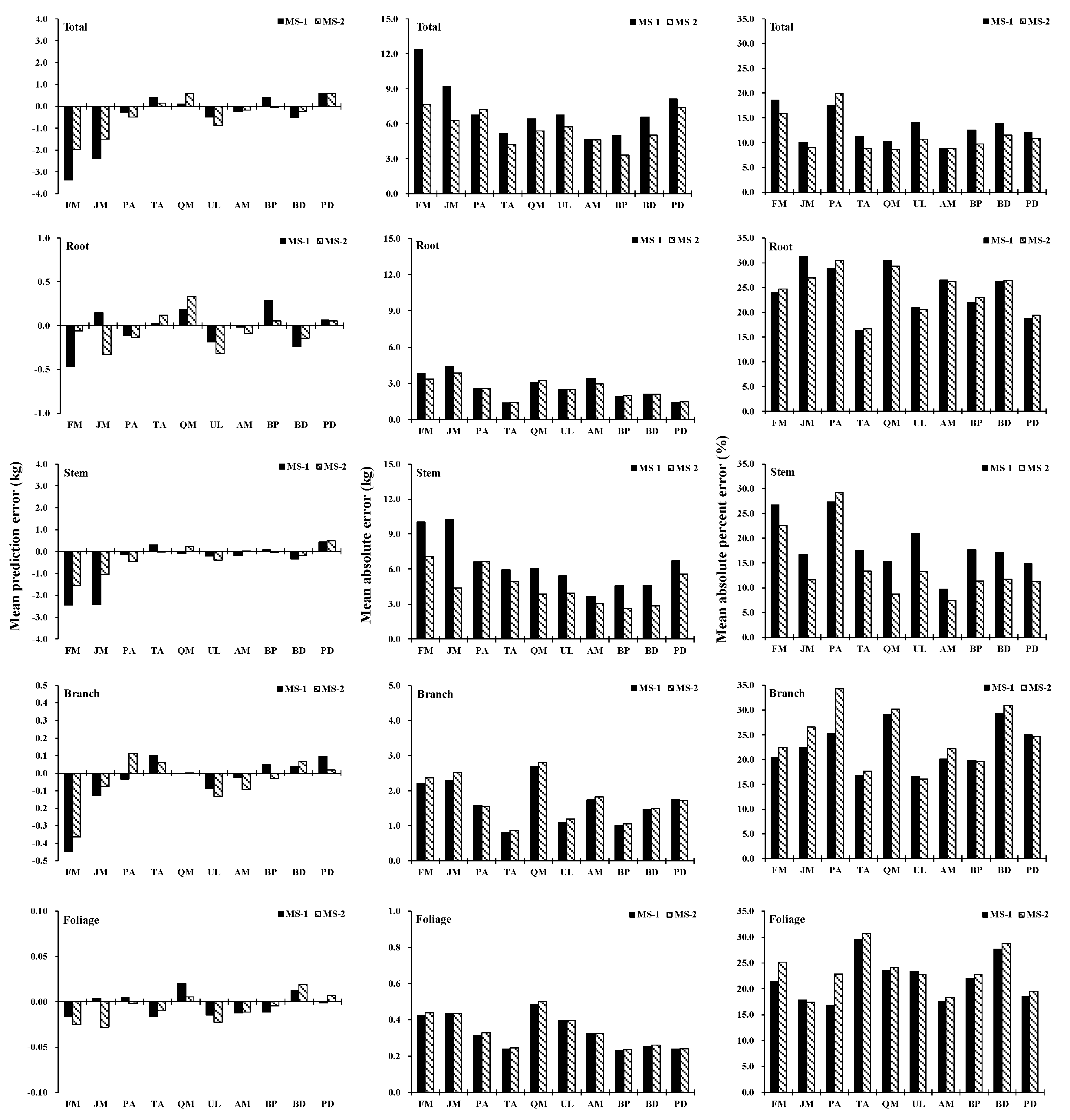
3.2. Allometric Equations of Carbon and Validation of Models

Under the NSUR method, two additive systems of carbon equations, one with D (Equation (6), namely MS-1) and the other with both D and H (Equation (7), namely MS-2) fit the carbon data of the 10 broadleaf species. The goodness-of-fit statistics (R_a² and RMSE) for each carbon equation suggested that all equations of MS-1 fit the carbon data well, with a R_a² > 87% and an RMSE < 17.5. The models fit the carbon data of the total and stem better, while a relatively smaller model R_a² value was observed in the root, branch, and foliage equations. Among the 10 broadleaf species, higher R_a² was detected in Phellodendron amurense and Betula platyphylla under the additive system with D (

Table 3. Model coefficient estimates, standard errors (SE), goodness-of-fit statistics, and weight functions for the additive system of biomass equations based on one predictor (D only, namely MS-1).

Tree Species	Carbon Components	βi0		βi1		${\mathit{R}}_{\mathit{a}}^2$	RMSE	Weight Function
		Estimate	SE	Estimate	SE
FM	Root	−4.3993	0.3836	2.5020	0.1221	0.9268	4.5548	D2.4537
	Stem	−2.2940	0.2322	2.1752	0.0753	0.9150	12.9900	D2.2577
	Branch	−6.2638	0.3550	2.9343	0.1114	0.9385	2.7533	D2.8112
	Foliage	−5.3096	0.4059	2.1160	0.1308	0.9307	0.5116	D2.1436
	Total	-	-	-	-	0.9431	17.4863	D2.2123
JM	Root	−3.4686	0.3393	2.0564	0.1068	0.8948	5.5046	D2.9440
	Stem	−3.6363	0.1651	2.5117	0.0547	0.9539	13.9442	D3.8552
	Branch	−4.2657	0.2768	2.2587	0.0839	0.9549	3.0605	D1.9283
	Foliage	−5.5766	0.2931	2.1833	0.0930	0.9677	0.5337	D3.2885
	Total	-	-	-	-	0.9808	13.4931	D3.4722
PA	Root	−6.4318	0.4733	3.0452	0.1441	0.9766	2.9545	D2.0757
	Stem	−3.3025	0.1385	2.3845	0.0417	0.9756	7.1162	D2.8811
	Branch	−6.2062	0.4173	2.8708	0.1273	0.9806	1.8019	D2.0720
	Foliage	−5.7706	0.4033	2.2266	0.1265	0.9644	0.4015	D2.7516
	Total	-	-	-	-	0.9895	8.1229	D2.9551
TA	Root	−3.2098	0.2114	1.9424	0.0721	0.9720	1.7613	D2.8887
	Stem	−3.5676	0.1580	2.4640	0.0501	0.9686	8.2212	D2.4344
	Branch	−5.7017	0.2577	2.5094	0.0853	0.9663	1.3210	D3.6814
	Foliage	−5.1279	0.3364	1.8247	0.1125	0.8780	0.3153	D2.3317
	Total	-	-	-	-	0.9870	7.3417	D1.9310
QM	Root	−4.1592	0.1892	2.3883	0.0621	0.9555	4.3850	D3.6476
	Stem	−3.0136	0.1422	2.3729	0.0451	0.9785	8.5595	D2.7019
	Branch	−6.6852	0.2577	3.1627	0.0797	0.9759	3.8246	D3.7733
	Foliage	−6.6988	0.2607	2.5843	0.0802	0.9489	0.7517	D2.1625
	Total	-	-	-	-	0.9922	9.3531	D2.5420
UL	Root	−3.2591	0.1909	2.0468	0.0643	0.9446	3.3534	D2.8270
	Stem	−2.6275	0.1185	2.1730	0.0374	0.9703	7.2734	D2.7464
	Branch	−3.2156	0.1607	1.8316	0.0535	0.9567	1.3939	D2.6379
	Foliage	−3.9191	0.2446	1.6018	0.0844	0.8991	0.4876	D2.6514
	Total	-	-	-	-	0.9805	8.9256	D2.8154
AM	Root	−4.8306	0.3060	2.6609	0.0965	0.9558	4.0845	D2.1791
	Stem	−2.8834	0.1263	2.3046	0.0409	0.9817	5.3065	D2.1708
	Branch	−4.2090	0.2139	2.3003	0.0724	0.9483	2.2505	D2.8763
	Foliage	−4.2266	0.1870	1.7472	0.0663	0.9218	0.4071	D2.9753
	Total	-	-	-	-	0.9905	6.7462	D2.4949
BP	Root	−4.0412	0.1659	2.3718	0.0583	0.9637	2.9315	D3.6368
	Stem	−2.7296	0.1158	2.2856	0.0407	0.9644	6.9291	D2.8397
	Branch	−6.0092	0.2256	2.8747	0.0760	0.9798	1.5945	D3.6122
	Foliage	−6.3597	0.1641	2.4766	0.0566	0.9714	0.3290	D3.0989
	Total	-	-	-	-	0.9876	7.1944	D2.3971
BD	Root	−3.8799	0.1525	2.2312	0.0518	0.9108	3.2188	D2.2107
	Stem	−3.1879	0.1703	2.4001	0.0599	0.9603	6.8378	D3.6068
	Branch	−8.3881	0.3189	3.6647	0.1025	0.9659	2.5285	D3.6079
	Foliage	−8.0584	0.2529	3.0287	0.0799	0.9793	0.3108	D1.4856
	Total	-	-	-	-	0.9715	10.1206	D3.6981
PD	Root	−4.3300	0.2395	2.2614	0.0762	0.9606	1.8136	D2.2476
	Stem	−2.8292	0.1402	2.2754	0.0463	0.9563	8.8689	D2.9923
	Branch	−7.5074	0.3793	3.1670	0.1185	0.9420	2.2657	D3.9500
	Foliage	−6.8948	0.2619	2.4573	0.0824	0.9300	0.3662	D2.2230
	Total	-	-	-	-	0.9673	11.1664	D2.5572

Note: FM: Fraxinus manshuric; JM: Juglans mandshurica; PA: Phellodendron amurense; QM: Quercus mongolica; TA: Tilia amurensis; UL: Ulmus laciniata; AM: Acer mono; BP: Betula platyphylla; BD: Betula davuria; PD: Populus davidiana.

). The carbon equation MS-2 was constructed with both D and H when the height of the tree was available. Compared with equation MS-1, equation MS-2 had a greater R_a² and smaller RMSE for most of the total, root, stem, branch, and foliage values (

Table 4. Model coefficient estimates, standard errors, goodness-of-fit statistics, and weight functions for the additive system of biomass equations based on two predictors (D and H, namely MS-2).

Tree Species	Carbon Components	βi0		βi1		βi2		${\mathit{R}}_{\mathit{a}}^2$	RMSE	Weight Function
		Estimate	SE	Estimate	SE	Estimate	SE
FM	Root	−3.9956	0.6335	2.2747	0.1376	0.1004	0.2629	0.9443	3.9741	D2.0463
	Stem	−3.2245	0.3059	1.6765	0.0607	0.8291	0.1256	0.9706	7.6390	D1.9876
	Branch	−7.3358	0.5465	2.8620	0.1254	0.4330	0.2388	0.9372	2.7832	D2.7448
	Foliage	−4.5477	0.6954	2.0263	0.1575	−0.1628	0.2959	0.9344	0.4978	D1.8113
	Total	-	-	-	-	-	-	0.9804	10.2714	D2.1491
JM	Root	−3.0664	0.4009	2.5876	0.1889	−0.7066	0.2311	0.9097	5.0990	D2.6508
	Stem	−3.9598	0.1280	1.8806	0.0593	0.7856	0.0707	0.9899	6.5391	D2.8925
	Branch	−3.8308	0.2301	2.2356	0.1147	−0.1199	0.1394	0.9585	2.9341	D1.7883
	Foliage	−5.4919	0.3287	2.3766	0.1565	−0.2361	0.1906	0.9679	0.5322	D2.7763
	Total	-	-	-	-	-	-	0.9915	8.9693	D2.6857
PA	Root	−6.2320	0.6971	2.9456	0.2139	0.0434	0.3526	0.9764	2.9710	D2.2485
	Stem	−3.0940	0.2925	2.4544	0.0915	−0.1513	0.1472	0.9755	7.1248	D2.2018
	Branch	−5.6096	0.6007	2.7677	0.1845	−0.0899	0.3022	0.9829	1.6899	D1.8890
	Foliage	−4.8826	0.4613	2.3390	0.2023	−0.4366	0.3015	0.9702	0.3678	D1.9366
	Total	-	-	-	-	-	-	0.9880	8.6846	D2.3215
TA	Root	−3.3346	0.3365	1.8780	0.1274	0.1138	0.2220	0.9699	1.8267	D3.0437
	Stem	−4.5319	0.2987	2.1628	0.0888	0.6881	0.1772	0.9774	6.9783	D2.4724
	Branch	−5.6928	0.4856	2.5542	0.1647	−0.0513	0.3005	0.9686	1.2752	D3.2538
	Foliage	−5.0719	0.5696	1.8170	0.2026	−0.0126	0.3619	0.8808	0.3117	D2.2758
	Total	-	-	-	-	-	-	0.9906	6.2356	D2.0373
QM	Root	−3.8662	0.2290	2.5715	0.0990	−0.3216	0.1586	0.9561	4.3558	D2.9477
	Stem	−3.9306	0.1226	2.0347	0.0426	0.7199	0.0695	0.9894	6.0027	D2.7199
	Branch	−6.6321	0.3426	3.1306	0.1060	0.0172	0.1639	0.9756	3.8468	D2.7882
	Foliage	−6.6655	0.3530	2.6626	0.1117	−0.1021	0.1702	0.9507	0.7381	D1.8370
	Total	-	-	-	-	-	-	0.9943	7.9764	D2.5228
UL	Root	−3.4129	0.2592	2.1852	0.1136	−0.0981	0.1772	0.9414	3.4469	D2.5519
	Stem	−3.8518	0.1737	1.9719	0.0592	0.6701	0.0903	0.9834	5.4327	D2.3251
	Branch	−3.2943	0.2284	1.9281	0.0923	−0.0789	0.1423	0.9503	1.4939	D2.2346
	Foliage	−3.8016	0.3880	1.7543	0.1647	−0.2134	0.2565	0.8935	0.5008	D2.1660
	Total	-	-	-	-	-	-	0.9838	8.1408	D2.2144
AM	Root	−3.9510	0.2955	2.7922	0.0853	−0.4747	0.1223	0.9641	3.6834	D1.7510
	Stem	−3.6194	0.1403	2.1589	0.0486	0.4375	0.0827	0.9867	4.5312	D2.6590
	Branch	−3.9286	0.3449	2.2380	0.1104	−0.0329	0.1789	0.9530	2.1452	D2.0332
	Foliage	−4.2369	0.3343	1.6296	0.1183	0.1351	0.2048	0.9270	0.3935	D2.2499
	Total	-	-	-	-	-	-	0.9906	6.7104	D2.3593
BP	Root	−4.0713	0.4800	2.3894	0.1698	−0.0005	0.2997	0.9668	2.8031	D3.2843
	Stem	−4.1802	0.1955	1.7812	0.0583	1.0230	0.1105	0.9902	3.6256	D2.5802
	Branch	−5.9972	0.7607	2.9277	0.2163	−0.0561	0.4189	0.9788	1.6346	D3.5408
	Foliage	−6.1326	0.3590	2.4996	0.0978	−0.1040	0.1938	0.9727	0.3215	D2.2578
	Total	-	-	-	-	-	-	0.9953	4.4225	D2.1757
BD	Root	−4.0287	0.2430	2.2069	0.1334	0.0778	0.1857	0.9122	3.1936	D2.3814
	Stem	−4.1736	0.1466	1.8585	0.0614	0.9411	0.0871	0.9864	3.9996	D3.1062
	Branch	−8.6425	0.4104	3.7298	0.1669	0.0178	0.2210	0.9692	2.4030	D3.3696
	Foliage	−8.1679	0.3071	3.0751	0.1215	−0.0133	0.1593	0.9799	0.3064	D1.2775
	Total	-	-	-	-	-	-	0.9826	7.9073	D3.3496
PD	Root	−4.3908	0.4537	2.1979	0.1090	0.0875	0.2109	0.9607	1.8118	D2.1666
	Stem	−4.1757	0.2161	1.9245	0.0594	0.8179	0.1128	0.9687	7.5064	D2.9923
	Branch	−7.0421	0.8779	3.3141	0.2075	−0.3094	0.4057	0.9426	2.2546	D3.2213
	Foliage	−6.1852	0.4526	2.5739	0.1114	−0.3613	0.2111	0.9338	0.3562	D2.1713
	Total	-	-	-	-	-	-	0.9722	10.3088	D2.1058

Note: FM: Fraxinus manshuric; JM: Juglans mandshurica; PA: Phellodendron amurense; QM: Quercus mongolica; TA: Tilia amurensis; UL: Ulmus laciniata; AM: Acer mono; BP: Betula platyphylla; BD: Betula davuria; PD: Populus davidiana.

).

Based on jackknifing residuals of the two carbon equation systems (MS-1 and MS-2), the model validations for Equations (10)–(12) were computed. For the total carbon, relatively small model prediction errors were reported for the two systems (−0.50 < MPE < 0.90, MAE < 9.0 kg, and MAB% < 19.0%), except for Fraxinus mandshurica and Juglans mandshurica. MS-2 seemed to perform better than MS-1, which was also true for the stem carbon (Figure 3). On the other hand, compared to the total and stem carbon, less accurate predictions were observed in the carbon equations for root, branch, and foliage (MAE% > 16%). The model performance was improved by adding H into the additive system of carbon equations for most of the 10 broadleaf species, but there were nonsignificant differences among the branches, foliage, and roots of some species (e.g., Ulmus laciniata, Phellodendron amurense, and Betula davurica) (Figure 3).

To quantify the spread of the observations of carbon, the residual and approximate confident bands of the observed data, containing approximately 90% of the average curve, were derived from all additive carbon equations. The specific methods for calculating the approximate confidence band were described by Bi et al. [28]. Compared to MS-1, the incorporation of H in MS-2 led to a slightly smaller confidence interval for carbon (Figure 4). In total, the carbon concentrations of all tissues from the 10 species of trees were predicted well with the equation systems, MS-1 and MS-2.

3.3. Carbon Partitioning

The relative ratio of stem to total tree carbon (Figure 5) was the largest in Populus davidiana (72.63 ± 2.92% (mean ± SD), followed by Fraxinus mandshurica (65.95 ± 4.51%) and Tilia amurensis (65.29 ± 5.21%), while the smallest was found in Acer mono (57.44 ± 2.29%). The largest proportion of root carbon was Tilia amurensis (23.37 ± 7.45%), followed by Ulmus laciniata (23.18 ± 1.82%) and Acer mono (22.90 ± 2.76%), where the smallest was for Populus davidiana (15.82 ± 1.45%). Compared with other tissues, the largest proportion of branch carbon was that of Acer mono (16.02 ± 2.94%), with the smallest in Tilia amurensis (8.78 ± 0.95%). The proportion of foliage carbon was the largest for Phellodendron amurense (3.77 ± 0.94%), and the smallest was for the Populus davidiana (2.16 ± 0.27%) (Figure 5). In general, the mean proportion of each carbon tissue was 63.68% for the stems, 20.79% for the roots, 12.50% for the branches, and 3.03% for the foliage. The carbon in the aboveground part (i.e., the sum of stem, foliage, and branch carbon) was approximately 79% of the total carbon, while that of the belowground (i.e., the roots) part was approximately 21.0% (Figure 5).

4. Discussion

The stability of biomass models is generally affected by factors related to tree growth, such as temperature and rainfall [7,43,44,45], which was also observed in the carbon model. Therefore, adding a wide range of natural variation to such factors is necessary when constructing the carbon model. In this study, the carbon concentrations of various tissue types of 10 broadleaf species and their variation with tree size were examined. When predicting individual tree carbon for the 10 broadleaf species in northeast China, the carbon concentrations and allometric equations were constructed from a dataset with a wide range of diameters and geographical locations, which made the prediction more accurate.

The carbon concentrations were significantly affected by the types and sizes of trees, along with the tissue types, which ranged from 42.47% in the root of Phellodendron amurense to 48.68% in the foliage of Betula platyphylla. The carbon concentration of the foliage was the highest, followed by that of the stem, branch, and root. The WMCC was the highest in Betula platyphylla and the lowest in Ulmus laciniata. This range of carbon concentration was more stable and narrower than that of the 11 Chinese temperate broadleaf species (48.36%–50.55%) [46], 8 other Chinese temperate broadleaf species in northeast China (43.70%–55.10%) [16], 41 tree species from North America (46.30%–55.20%) [47], and 32 tree species in tropical forests (44.40%–49.40%) [21]. Although the carbon was estimated by assuming the biomass carbon as a constant 50% (or other values) [48,49,50], the average carbon concentration of all tissues of all 10 broadleaf species (44.84%) in this study was smaller than the generic carbon concentration of 50%. Thus, it is inappropriate to calculate the carbon concentrations of the 10 broadleaf tree species in northeast China at 50%, and species-specific mean carbon concentrations of tissues or the WMCC should be used [10,16]. As tree sizes affected the carbon concentrations, the carbon concentrations of the branch, foliage, stem, and root samples of different tree sizes were also taken into consideration when calculating accurate individual tree carbon results [10]. In this study, the carbon of each tissue was the product of the multiplication of the carbon concentration by the biomass of each tissue. The sum of branch, foliage, stem, and root carbon produced the total tree carbon.

To predict the individual tree carbon, only those variables of the tree that were easy to measure in the field were used. Based on power-law models, the introduction of the typical allometric equations is used to increase carbon estimation accuracy in most studies. Concerning the allometric equations, D is an indispensable predictor of carbon models and forest growth. In practice, individual tree carbon models constructed with only D are simple and only require basic forest inventory data for the application [4,24,29,51]. Our results showed that D was the primary explanatory variable in the allometry model, resulting in the discrepancy between the total and tissue carbon. This may originate from the intimate correlations between tissues and diameter, which constitutes the overwhelming majority of total carbon in stems [4,9,29]. Nevertheless, relatively large variations appeared among the tissue types and the total carbon values with a given D, which reminded us that it was insufficient to predict the total or tissue carbon of the trees with the carbon model only constructed with D. To improve the predictive accuracy of the carbon equations, another variable was added. In order to reduce the biased estimates of carbon or biomass, the height of the tree is considered as another commonly used predictor variable by many scholars [24,25,29,33]. Dong et al. [24] also considered the tree height at different sites as a vital predictor variable to improve the carbon estimates of forests. This was the first study on the carbon equations of 10 broadleaf species in northeast China. In this study, the tree carbon data of a relatively large geographical area in northeast China were collected, and C = β₀D^β₁ and C = β₀D^β₁H^β₂ were selected to construct the basic equations that simulate the carbon allometric relationships of individual trees. Two carbon equation systems, MS-1 and MS-2, were constructed and tested with a jackknifing technique. The addition of H to the carbon equation improved the accuracy of the carbon equations of the 10 broadleaf species, which was reported in previous studies [24,25,29,33]. Overall, to acquire accurate carbon measurements of individual trees, the carbon allometric equation constructed with the whole, detailed data on the biomass and carbon concentration was the best [10,22].

Parresol [31] pointed out that the aggregation approach is the standard method for ensuring the additivity of carbon estimates, which can be used with various types of tree tissue. In the Parresol method, a nonlinear model is assigned to each of the N carbon tissues before aggregating these tissue models into the total tree carbon. Considering the intrinsic correlation among the tree tissues from the same sample tree, these aggregate models are typically estimated by weighted NSUR jointly to fit all N + 1 equations [29,30,31,33,34]. However, some nonadditive carbon equations are still published because of the use of least squares regression (OLS) of estimation [9,22,23].

Carbon partitioning plays a vital role in the future. In this study, there were strikingly noticeable differences in the carbon proportions of different tree tissues. According to the previous reports, the proportion of stem carbon is the largest, and branch and foliage carbon constitute a small amount of the total [10,22,23]. The average proportion of stem carbon of the 10 broadleaf species remained steady among the tree species, while the average proportion of branch carbon varied significantly. The phenomenon that some species, such as Populus davidiana, distributed more carbon to the stems (72.63%) than the roots (15.82%) mainly resulted from a small crown in the canopy and shallow lateral roots. In summary, the percentage of branch carbon varied across species, which probably resulted from the thickness of the branches and the formation of the forks. In the same way, the partitioning profiles of roots might also be linked with morphology of the tree root (e.g., deep or shallow roots), soil conditions, and growth processes [4,52,53]. The partitioning variation of the total carbon for tree tissues across the tree species has been reported in many studies, indicating that aboveground carbon generally occupies approximately 80% with the remaining 20% attributed to belowground carbon [10,22,23]. In this study, the proportions of stem and root carbon of the 10 broadleaf species exhibited approximately 64% and 21%, respectively, of the total carbon for an average tree.

The difficulty in measuring the carbon in roots leads to scarce reports on root carbon. The difficulty in excavating tree roots was mainly because of the morphology of the tree roots and soil conditions. For some species, the usage of a chain (i.e., lifting equipment) can pull out coarse roots (diameter ≥ 2 cm) successfully. In our study, the prediction accuracy of the branch and leaf carbon equations was relatively low, probably because the 3–5 randomly selected branches of each crown layer led to a large variation. Therefore, increasing the number of separated branch samples in the future may improve the prediction accuracy of the branch and foliage carbon equations, as separating and weighing all the branches is time-consuming and hard to accomplish.

In summary, accurately estimating the carbon of large trees is critical for the estimation of forest carbon, because large trees usually retain a high proportion of the carbon in forests. The maximum diameters of the 10 species in this study ranged from 30.0 cm to 41.1 cm, which made the prediction of the carbon in the forest of northeast China feasible. However, if the carbon equations of this study are used to estimate individual tree carbon outside of this data, the models may produce uncertain prediction errors.

5. Conclusions

When estimating individual tree carbon, the significance of variation in carbon concentration was addressed in this study, and meant a lot in validating the global carbon accounting and the model used. The carbon concentration of the foliage was notably higher than that of the other tissues, which varied among the 10 broadleaf species. The carbon models constructed with the predictor variables D and H explained the variation of the 10 broadleaf species. As expected, different accuracies of the two additive carbon equations of the 10 broadleaf species were detected, and MS-2 had better goodness-of-fit and validation statistics than MS-1. For the carbon equations of total tissue and stem, the RMSE of the model was relatively larger than that for the roots, branches, and foliage. Overall, adding H to the carbon equations strikingly improved the performance and model fit.

The carbon partitioning of aboveground and belowground tissues of the 10 broadleaf species conforms with the other reports, in which stem carbon contains the majority of the total carbon. The tree carbon data of this study were in a wide range of geographical locations and diameter grades. Therefore, the species-specific allometric models of this study enhance the prediction of aboveground and belowground carbon of the same tree species in different locations and supplies basic information to the Chinese National Forest Inventory.

References

1. FAO. FAO Statistical Yearbook: World Food and Agriculture; FAO: Rome, Italy, 2013. [Google Scholar]
2. Canadell, J.G.; Le Quéré, C.; Raupach, M.R.; Field, C.B.; Buitenhuis, E.T.; Ciais, P.; Conway, T.J.; Gillett, N.P.; Houghton, R.; Marland, G. Contributions to accelerating atmospheric CO2 growth from economic activity, carbon intensity, and efficiency of natural sinks. Proc. Natl. Acad. Sci. USA 2007, 104, 18866–18870. [Google Scholar] [CrossRef]
3. Pan, Y.; Birdsey, R.A.; Fang, J.; Houghton, R.; Kauppi, P.E.; Kurz, W.A.; Phillips, O.L.; Shvidenko, A.; Lewis, S.L.; Canadell, J.G. A large and persistent carbon sink in the world’s forests. Science 2011, 333, 988–993. [Google Scholar] [CrossRef]
4. Wang, C. Biomass allometric equations for 10 co-occurring tree species in Chinese temperate forests. For. Ecol. Manag. 2006, 222, 9–16. [Google Scholar] [CrossRef]
5. State Forestry Administration the Eighth Forest Resource Survey Report. 2014. Available online: http://211.167.243.162:8085/8/index.html (accessed on 14 October 2019).
6. Canadell, J.G.; Raupach, M.R. Managing forests for climate change mitigation. Science 2008, 320, 1456–1457. [Google Scholar] [CrossRef]
7. Foster, J.R.; Finley, A.O.; D’amato, A.W.; Bradford, J.B.; Banerjee, S. Predicting tree biomass growth in the temperate–boreal ecotone: Is tree size, age, competition, or climate response most important? Glob. Chang. Biol. 2016, 22, 2138–2151. [Google Scholar] [CrossRef]
8. Kachamba, D.; Eid, T.; Gobakken, T. Above-and belowground biomass models for trees in the miombo woodlands of Malawi. Forests 2016, 7, 38. [Google Scholar] [CrossRef]
9. Kapinga, K.; Syampungani, S.; Kasubika, R.; Yambayamba, A.M.; Shamaoma, H. Species-specific allometric models for estimation of the above-ground carbon stock in miombo woodlands of Copperbelt Province of Zambia. For. Ecol. Manag. 2018, 417, 184–196. [Google Scholar] [CrossRef]
10. Dong, L.; Zhang, L.; Li, F. Allometry and partitioning of individual tree biomass and carbon of Abies nephrolepis Maxim in northeast China. Scand. J. For. Res. 2016, 31, 399–411. [Google Scholar] [CrossRef]
11. Gower, S.T.; Kucharik, C.J.; Norman, J.M. Direct and indirect estimation of leaf area index, fAPAR, and net primary production of terrestrial ecosystems. Remote Sens. Environ. 1999, 70, 29–51. [Google Scholar] [CrossRef]
12. Losi, C.J.; Siccama, T.G.; Condit, R.; Morales, J.E. Analysis of alternative methods for estimating carbon stock in young tropical plantations. For. Ecol. Manag. 2003, 184, 355–368. [Google Scholar] [CrossRef]
13. Neumann, M.; Moreno, A.; Mues, V.; Härkönen, S.; Mura, M.; Bouriaud, O.; Lang, M.; Achten, W.M.; Thivolle-Cazat, A.; Bronisz, K. Comparison of carbon estimation methods for European forests. For. Ecol. Manag. 2016, 361, 397–420. [Google Scholar] [CrossRef]
14. Houghton, R.A. Converting terrestrial ecosystems from sources to sinks of carbon. Ambio 1996, 25, 267–272. [Google Scholar]
15. Gower, S.; Krankina, O.; Olson, R.; Apps, M.; Linder, S.; Wang, C. Net primary production and carbon allocation patterns of boreal forest ecosystems. Ecol. Appl. 2001, 11, 1395–1411. [Google Scholar] [CrossRef]
16. Zhang, Q.; Wang, C.; Wang, X.; Quan, X. Carbon concentration variability of 10 Chinese temperate tree species. For. Ecol. Manag. 2009, 258, 722–727. [Google Scholar] [CrossRef]
17. Castaño-Santamaría, J.; Bravo, F. Variation in carbon concentration and basic density along stems of sessile oak (Quercus petraea (Matt.) Liebl.) and Pyrenean oak (Quercus pyrenaica Willd.) in the Cantabrian Range (NW Spain). Ann. For. Sci. 2012, 69, 663–672. [Google Scholar] [CrossRef]
18. Wang, X.W.; Weng, Y.H.; Liu, G.F.; Krasowski, M.J.; Yang, C.P. Variations in carbon concentration, sequestration and partitioning among Betula platyphylla provenances. For. Ecol. Manag. 2015, 358, 344–352. [Google Scholar] [CrossRef]
19. Martin, A.R.; Gezahegn, S.; Thomas, S.C. Variation in carbon and nitrogen concentration among major woody tissue types in temperate trees. Can. J. For. Res. 2015, 45, 744–757. [Google Scholar] [CrossRef]
20. Gao, B.; Taylor, A.R.; Chen, H.Y.; Wang, J. Variation in total and volatile carbon concentration among the major tree species of the boreal forest. For. Ecol. Manag. 2016, 375, 191–199. [Google Scholar] [CrossRef]
21. Elias, M.; Potvin, C. Assessing inter-and intra-specific variation in trunk carbon concentration for 32 neotropical tree species. Can. J. For. Res. 2003, 33, 1039–1045. [Google Scholar] [CrossRef]
22. Mello, A.A.D.; Nutto, L.; Weber, K.S.; Sanquetta, C.E.; Matos, J.L.M.D.; Becker, G. Individual biomass and carbon equations for Mimosa scabrella Benth. (Bracatinga) in Southern Brazil. Silva Fenn. 2012, 46, 333–343. [Google Scholar] [CrossRef]
23. Zhu, H.; Weng, Y.; Zhang, H.; Meng, F.; Major, J. Comparing fast-and slow-growing provenances of Picea koraiensis in biomass, carbon parameters and their relationships with growth. For. Ecol. Manag. 2013, 307, 178–185. [Google Scholar] [CrossRef]
24. Dong, L.; Zhang, L.; Li, F. Additive biomass equations based on different dendrometric variables for two dominant species (Larix gmelini Rupr. and Betula platyphylla Suk.) in natural forests in the eastern Daxing’an Mountains, Northeast China. Forests 2018, 9, 261. [Google Scholar] [CrossRef]
25. Zhao, D.; Kane, M.; Markewitz, D.; Teskey, R.; Clutter, M. Additive tree biomass equations for midrotation loblolly pine plantations. For. Sci. 2015, 61, 613–623. [Google Scholar] [CrossRef]
26. Kralicek, K.; Huy, B.; Poudel, K.P.; Temesgen, H.; Salas, C. Simultaneous estimation of above-and below-ground biomass in tropical forests of Viet Nam. For. Ecol. Manag. 2017, 390, 147–156. [Google Scholar] [CrossRef]
27. Zhou, X.; Brandle, J.R.; Schoeneberger, M.M.; Awada, T. Developing above-ground woody biomass equations for open-grown, multiple-stemmed tree species: Shelterbelt-grown Russian-olive. Ecol. Model. 2007, 202, 311–323. [Google Scholar] [CrossRef] [Green Version]
28. Bi, H.; Murphy, S.; Volkova, L.; Weston, C.; Fairman, T.; Li, Y.; Law, R.; Norris, J.; Lei, X.; Caccamo, G. Additive biomass equations based on complete weighing of sample trees for open eucalypt forest species in south-eastern Australia. For. Ecol. Manag. 2015, 349, 106–121. [Google Scholar] [CrossRef]
29. Dong, L.; Zhang, L.; Li, F. A three-step proportional weighting system of nonlinear biomass equations. For. Sci. 2015, 61, 35–45. [Google Scholar] [CrossRef]
30. Parresol, B.R. Assessing tree and stand biomass: A review with examples and critical comparisons. For. Sci. 1999, 45, 573–593. [Google Scholar]
31. Parresol, B.R. Additivity of nonlinear biomass equations. Can. J. For. Res. 2001, 31, 865–878. [Google Scholar] [CrossRef]
32. Tang, S.; Li, Y.; Wang, Y. Simultaneous equations, error-in-variable models, and model integration in systems ecology. Ecol. Model. 2001, 142, 285–294. [Google Scholar] [CrossRef]
33. Bi, H.; Turner, J.; Lambert, M.J. Additive biomass equations for native eucalypt forest trees of temperate Australia. Trees 2004, 18, 467–479. [Google Scholar] [CrossRef]
34. Zhao, D.; Westfall, J.; Coulston, J.W.; Lynch, T.B.; Bullock, B.P.; Montes, C.R. Additive biomass equations for slash pine trees: Comparing three modeling approaches. Can. J. For. Res. 2019, 49, 27–40. [Google Scholar] [CrossRef]
35. Finney, D. On the distribution of a variate whose logarithm is normally distributed. Suppl. J. R. Stat. Soc. 1941, 7, 155–161. [Google Scholar] [CrossRef]
36. Baskerville, G. Use of logarithmic regression in the estimation of plant biomass. Can. J. For. Res. 1972, 2, 49–53. [Google Scholar] [CrossRef]
37. Clifford, D.; Cressie, N.; England, J.R.; Roxburgh, S.H.; Paul, K.I. Correction factors for unbiased, efficient estimation and prediction of biomass from log–log allometric models. For. Ecol. Manag. 2013, 310, 375–381. [Google Scholar] [CrossRef]
38. Zianis, D.; Xanthopoulos, G.; Kalabokidis, K.; Kazakis, G.; Ghosn, D.; Roussou, O. Allometric equations for aboveground biomass estimation by size class for Pinus brutia Ten. Trees growing in North and South Aegean Islands, Greece. Eur. J. For. Res. 2011, 130, 145–160. [Google Scholar] [CrossRef]
39. Dong, L.; Zhang, L.; Li, F. A compatible system of biomass equations for three conifer species in Northeast, China. For. Ecol. Manag. 2014, 329, 306–317. [Google Scholar] [CrossRef]
40. Meng, S.; Liu, Q.; Zhou, G.; Jia, Q.; Zhuang, H.; Zhou, H. Aboveground tree additive biomass equations for two dominant deciduous tree species in Daxing’anling, northernmost China. J. For. Res. 2017, 22, 233–240. [Google Scholar] [CrossRef]
41. Paul, K.I.; Radtke, P.J.; Roxburgh, S.H.; Larmour, J.; Waterworth, R.; Butler, D.; Brooksbank, K.; Ximenes, F. Validation of allometric biomass models: How to have confidence in the application of existing models. For. Ecol. Manag. 2018, 412, 70–79. [Google Scholar] [CrossRef]
42. SAS Institute Inc. SAS/ETS 9.3 User’s Guide; SAS Institute Inc.: Cary, NC, USA, 2011. [Google Scholar]
43. Chave, J.; Réjou-Méchain, M.; Búrquez, A.; Chidumayo, E.; Colgan, M.S.; Delitti, W.B.; Duque, A.; Eid, T.; Fearnside, P.M.; Goodman, R.C. Improved allometric models to estimate the aboveground biomass of tropical trees. Glob. Chang. Biol. 2014, 20, 3177–3190. [Google Scholar] [CrossRef]
44. Fu, L.; Sun, W.; Wang, G. A climate-sensitive aboveground biomass model for three larch species in northeastern and northern China. Trees 2017, 31, 557–573. [Google Scholar] [CrossRef]
45. Zeng, W.; Duo, H.; Lei, X.; Chen, X.; Wang, X.; Pu, Y.; Zou, W. Individual tree biomass equations and growth models sensitive to climate variables for Larix spp. in China. Eur. J. For. Res. 2017, 136, 233–249. [Google Scholar] [CrossRef]
46. Thomas, S.; Malczewski, G. Wood carbon content of tree species in Eastern China: Interspecific variability and the importance of the volatile fraction. J. Environ. Manag. 2007, 85, 659–662. [Google Scholar] [CrossRef]
47. Lamlom, S.; Savidge, R. A reassessment of carbon content in wood: Variation within and between 41 North American species. Biomass Bioenergy 2003, 25, 381–388. [Google Scholar] [CrossRef]
48. Ngo, K.M.; Turner, B.L.; Muller-Landau, H.C.; Davies, S.J.; Larjavaara, M.; bin Nik Hassan, N.F.; Lum, S. Carbon stocks in primary and secondary tropical forests in Singapore. For. Ecol. Manag. 2013, 296, 81–89. [Google Scholar] [CrossRef]
49. Zhang, Y.; Gu, F.; Liu, S.; Liu, Y.; Li, C. Variations of carbon stock with forest types in subalpine region of southwestern China. For. Ecol. Manag. 2013, 300, 88–95. [Google Scholar] [CrossRef]
50. Diédhiou, I.; Diallo, D.; Mbengue, A.; Hernandez, R.; Bayala, R.; Diémé, R.; Diédhiou, P.; Sène, A. Allometric equations and carbon stocks in tree biomass of Jatropha curcas L. in Senegal’s Peanut Basin. Glob. Ecol. Conserv. 2017, 9, 61–69. [Google Scholar] [CrossRef]
51. Jenkins, J.C.; Chojnacky, D.C.; Heath, L.S.; Birdsey, R.A. National-scale biomass estimators for United States tree species. For. Sci. 2003, 49, 12–35. [Google Scholar]
52. Strong, W.; Roi, G.L. Root-system morphology of common boreal forest trees in Alberta, Canada. Can. J. For. Res. 1983, 13, 1164–1173. [Google Scholar] [CrossRef]
53. Canadell, J.; Jackson, R.; Ehleringer, J.; Mooney, H.; Sala, O.; Schulze, E.-D. Maximum rooting depth of vegetation types at the global scale. Oecologia 1996, 108, 583–595. [Google Scholar] [CrossRef]
Figure 1. Geographical position of study area and sampling plots in Heilongjiang province.
Forests 10 00928 g001
Figure 2. Boxplots of diameter at breast height (D), total tree height (H), total biomass, and carbon for 10 tree species. Numbers on the right-hand side indicate the number of sample trees. FM: Fraxinus manshuric; JM: Juglans mandshurica; PA: Phellodendron amurense; QM: Quercus mongolica; TA: Tilia amurensis; UL: Ulmus laciniata; AM: Acer mono; BP: Betula platyphylla; BD: Betula davuria; PD: Populus davidiana.
Forests 10 00928 g002
Figure 3. Mean prediction error (MPE), mean absolute error (MAE), and mean absolute percent error (MAE%) among the total and component biomass for the 10 tree species. FM: Fraxinus manshuric; JM: Juglans mandshurica; PA: Phellodendron amurense; QM: Quercus mongolica; TA: Tilia amurensis; UL: Ulmus laciniata; AM: Acer mono; BP: Betula platyphylla; BD: Betula davuria; PD: Populus davidiana.
Forests 10 00928 g003
Figure 4. Multi-panel display of observed total, stem, and root carbon for 10 tree species plotted against their predicted values from MS-1 and MS-2. The diagonal line of unity is shown together with the 90% upper and lower confidence limits of prediction error in each panel. FM: Fraxinus manshuric; JM: Juglans mandshurica; PA: Phellodendron amurense; QM: Quercus mongolica; TA: Tilia amurensis; UL: Ulmus laciniata; AM: Acer mono; BP: Betula platyphylla; BD: Betula davuria; PD: Populus davidiana.
Forests 10 00928 g004
Figure 5. Distribution of aboveground and belowground carbon among different tree tissues (root, stem, branch, and foliage) for 432 trees from 10 tree species. FM: Fraxinus manshuric; JM: Juglans mandshurica; PA: Phellodendron amurense; QM: Quercus mongolica; TA: Tilia amurensis; UL: Ulmus laciniata; AM: Acer mono; BP: Betula platyphylla; BD: Betula davuria; PD: Populus davidiana.
Forests 10 00928 g005