Boreal Forests of Kamchatka: Structure and Composition

Abstract

Central Kamchatka abounds in virgin old-growth boreal forest, formed primarily by Larix cajanderi and Betula platyphylla in varying proportions. A series of eight 0.25–0.30 ha plots captured the range of forests present in this region and their structure is described. Overall trends in both uplands and lowlands are for higher sites to be dominated by L. cajanderi with an increasing component of B. platyphylla with decreasing altitude. The tree line on wet sites is commonly formed by mono-dominant B. ermanii forests. Basal area ranged from 7.8–38.1 m²/ha and average tree height from 8.3–24.7 m, both being greater in lowland forests. Size distributions varied considerably among plots, though they were consistently more even for L. cajanderi than B. platyphylla. Upland sites also contained a dense subcanopy of Pinus pumila averaging 38% of ground area. Soil characteristics differed among plots, with upland soils being of lower pH and containing more carbon. Comparisons are drawn with boreal forests elsewhere and the main current threats assessed. These forests provide a potential baseline to contrast with more disturbed regions elsewhere in the world and therefore may be used as a target for restoration efforts or to assess the effects of climate change independent of human impacts.

1. Introduction

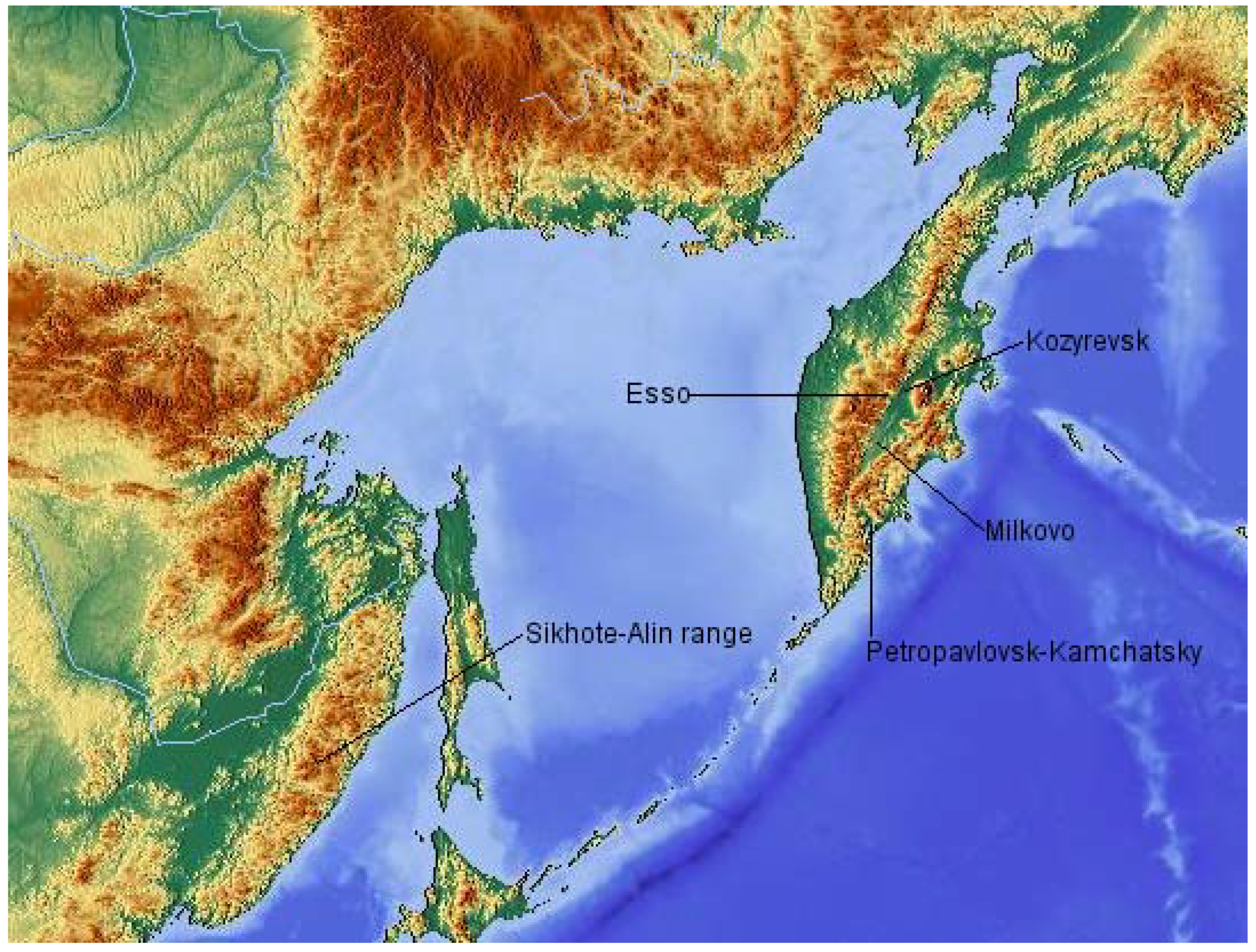
The boreal zone contains approximately one third of global forests, with 22% in Russia alone [1]. The Kamchatka peninsula lies on the extreme eastern fringe of Russia. Due to its remoteness and the strict controls on entry applied to both Russian nationals and foreigners for most of the past century, its vegetation has remained poorly described. In the international literature the principle source of information remains the flora produced by Eric Hulten [2] based on expeditions a century ago, and the region is considered to have a poor level of floristic knowledge [3] despite recent efforts to produce more up-to-date and accessible accounts for the Russian Far East as a whole [4] or Kamchatka itself [5,6]. This is most apparent in the central mountainous regions which were not visited by Hulten and comprise their own distinct ecoregion [7]. A major factor in the paucity of information has been the tendency for Russian scientists to publish their research in regional outlets with limited circulation [4].

At a time of increasing threats to forested ecosystems globally, Kamchatka presents an ideal opportunity for the study of forests which have suffered remarkably limited human impacts. The peninsula remains 88% forested, whilst almost 80% of its population live in the limited area of the regional capital (Petropavlovsk-Kamchatsky) and the nearby town of Yelizovo [8]. Timber extraction was formerly destructive, especially within the central conifer-dominated region of Kamchatka, where only an estimated 2.1% (350,000 ha) remains undisturbed by logging or recent fire. Nevertheless, the timber industry is currently in abatement, and partially-logged forests have not been converted to alternative use but for the most part are regenerating.

As a consequence of the substantial tranches of intact vegetation, several recent schemes have identified the Kamchatka peninsula and its forests as a global priority region for conservation [9,10].The Bystrinsky region of central Kamchatka has been designated an UNESCO World Heritage Site on the basis of both its pristine environments and the Eveni people who settled the region in the early 18^th century as reindeer herders [8]. Almost a third of Kamchatka’s forests receive some protection from exploitation, though the Bystrinsky region remains threatened by potential mining developments and a lack of effective legal safeguards [8].

According to figures presented by Krestov [4], the forests of Kamchatka are dominated by Betula ermanii Cham. (5,781.6 Mha), with extensive tracts of Larix cajanderi Mayr (951.3 Mha) and Betula platyphylla Sukacz. (641.7 Mha). The predominance of the former and relative scarcity of the latter set Kamchatka apart within the region. To some extent the latter two forest types have benefitted from declines in the area of Picea ajanensis (Lindl. Ex Gord.) Fisch. ex Carr (now 201.1 Mha) due to logging. The northern half of the peninsula and montane regions elsewhere are dominated by Pinus pumila (Pall.) Regel (8062.1 Mha), while wet sites typically support short-stature forests dominated by Salix spp. (311.0 Mha) or Alnus fruticosa Pall. (167.6 Mha), and a gallery forest of Populus suaveolens Fisch. s. l. (168.3 Mha) is commonly associated with rivers. Plantations remain relatively scarce on the peninsula, although there are a number of regions where Pinus sylvestris L. has been introduced as a timber tree (6.3 Mha).

The biogeographical position of the peninsula makes for an intriguing comparison with the better-studied boreal forest regions in North America [11,12] and northern Europe [e.g., 13]. The dark taiga forests of Central Siberia have also received detailed treatment [14]. By contrast, relatively few ecological studies have been conducted in Kamchatkan forests [e.g., 15,16], and these have mostly been in secondary forests. In recent years a focus of local botanical research has been to unite the disparate classification schemes used to describe vegetation communities into the Braun-Blanquet scheme [4,6], while statistical community analyses have yet to be undertaken.

The forests of North America and Far East Russia have been separated since the late Tertiary, with the Bering Straits forming approximately 5.32 Ma [17], and as a result they share no tree species; indeed, even congeneric species on either side of the North Pacific have markedly different ecological and ecophysiological attributes [18]. It would appear that much of Beringia and the Kamchatka peninsula were not fully glaciated at the Last Glacial Maximum, making it a potential refugium for many species [19], some of which have persisted into the Holocene. Both Picea ajanensis and Abies gracilis Kom. (=Abies sachalinensis Fr. Schmidt) occur in isolated forests on the peninsula, over 2,000 km from their present ranges [6]. Moreover, the extent of ice further north would have effectively sealed Kamchatkan species from mainland populations. Its 29 active volcanoes are expected to have profound impacts on soil characteristics, while a maritime climate buffers against the extreme winters experienced by continental Eurasia, and with characteristically mild and foggy weather throughout the summer [6].

The most common disturbances in East Eurasian boreal forests are crown and surface fires, and mass defoliation by insects, with gap-phase dynamics being relatively unimportant, some arguing that they do not develop unless forests remain unburnt for over 1,000 years [20]. Due to greater flammability the light taiga has a higher frequency of fires [20], which in North American forests is thought to allow light-demanding species to persist in the landscape [12]. The annual area of forest fires in Russia has been increasing over recent years, of which a large proportion can be attributed to human activity [1], though climate change is likely to be a contributing factor. The Kamchatka peninsula lies in a region where global temperatures are thought to have been rising rapidly, though a lack of long-term weather datasets in the region makes it difficult to ascertain the severity of these changes. One of the few available datasets, from Esso, in the central part of the peninsula, shows that temperatures have been increasing since the 1920s [21]. There is therefore an opportunity to assess the impacts of climatic change upon a largely intact and contiguous tract of boreal vegetation. Boreal forests contain approximately 27% of global vegetation carbon and 28% of global soil carbon, but have also been burning at an increased rate in recent decades [22,23]. This makes them a critical battleground in combating global climate change [1].

An expedition to the central region of Kamchatka was conducted in 2008 with the aim of establishing a series of permanent monitoring plots within each of the major forms of central Kamchatkan forests. Here I present details of their structure and composition and place them within the regional landscape context. It is hoped that drawing attention to these valuable ecological resources will inspire and inform future studies.

2. Experimental Section

2.1. Study Site and Species

Fieldwork was based around the village of Esso (55° 55.638 N, 158° 42.184 E) and an abandoned village in the Central Depression (54° 48.022 N, 159° 30.633 E); see Figure 1. Local forests are dominated by three tree species: Betula platyphylla, Larix cajanderi and B. ermanii. The first two exist as dominants or in fully-mixed forests, while the latter forms exclusive forests at the tree line on wet sites. In some areas Populus tremula L. forms a major component, especially in regenerating stands or on steep and rocky slopes. Other abundant elements are the shrubby species Alnus fruticosa and Pinus pumila which form a sub-canopy in montane forests and dominate on some upland sites. On inundated soils and along rivers a gallery forest of Populus suaveolens forms; this was not considered in the present study. Although a few trees of Picea ajanensis were found in domestic gardens in the village of Esso, the species is absent from local forests, though it occurs naturally in the Central Depression of Kamchatka [24,25]. The forest altitudinal limit is around 800 m [24].

Figure 1. Regional map of Far East Russia with locations referred to in the text.

Figure 1. Regional map of Far East Russia with locations referred to in the text.

In Esso valley permafrost is sporadic and discontinuous with a lower limit between 400–900 m above sea level (asl) [26]. Climatic data (1940–1995) suggest a mean annual temperature (MAT) of −3.1 °C, ranging from a minimum monthly mean in January of −18.7 °C to a maximum in July of 13.2 °C. Annual precipitation is 398 mm p.a. The closest data records to the lowland study site are from Kozyrevsk (MAT −1.8 °C, January −19.2 °C, July 15.1 °C, 512 mm pa) and Milkovo (MAT −2.7 °C, January −21.8 °C, July 15.0 °C, 540 mm p.a.) [6], indicating a relatively consistent climate across this region.

2.2. Plot Location and Establishment

Eight plots were established in 2008 to capture the range of forest types present in central Kamchatka (Table 1). Plots were selected on the basis of random GPS co-ordinates from within contiguous and homogeneous forest patches of at least 1 km² in size. They were chosen as those exhibiting minimal signs of human impact and for which no records of exploitation were held by Bystrinsky Nature Park. Extensive perambulations confirmed that plots were representative. Three lowland plots were selected to represent forests dominated by L. cajanderi, B. platyphylla or mixed. Three montane plots were selected with the same criteria, with a duplicate plot dominated by L. cajanderi. One further plot was established in forest dominated by B. ermanii.

Table 1. Characteristics of old-growth forest plots in Central Kamchataka. Dominant tree species are determined on the basis of importance values exceeding 20 (see Table 3); Lc = Larix cajanderi, Bp = Betula platyphylla, Be = Betula ermanii.

Location	Plot	Dominant species	Size (ha)	Altitude (m asl)	Slope	Facing	Co-ordinates
Lowland	1	Lc/Bp	0.25	108	0°	na	55° 49’ 678 N, 159° 28’ 987 E
	2	Bp/Lc	0.25	72	1°	na	55° 49’ 009 N, 159° 31’ 003 E
	3	Bp	0.25	64	0°	na	55° 48’ 036 N, 159° 33’ 091 E
Upland	1	Lc	0.30	700	10°	241°	55° 59’ 659 N, 158° 44’ 432 E
	2	Lc	0.25	591	1°	na	56° 04’ 431 N, 158° 54’ 222 E
	3	Lc/Bp	0.30	547	7°	145°	55° 59’ 031 N, 158° 45’ 059 E
	4	Bp	0.25	665	5°	190°	55° 51’ 679 N, 158° 38’ 242 E
	5	Be	0.25	700	15°	155°	55° 52’ 532 N, 158° 37’ 789 E

Table 1. Characteristics of old-growth forest plots in Central Kamchataka. Dominant tree species are determined on the basis of importance values exceeding 20 (see Table 3); Lc = Larix cajanderi, Bp = Betula platyphylla, Be = Betula ermanii.

Location	Plot	Dominant species	Size (ha)	Altitude (m asl)	Slope	Facing	Co-ordinates
Lowland	1	Lc/Bp	0.25	108	0°	na	55° 49’ 678 N, 159° 28’ 987 E
	2	Bp/Lc	0.25	72	1°	na	55° 49’ 009 N, 159° 31’ 003 E
	3	Bp	0.25	64	0°	na	55° 48’ 036 N, 159° 33’ 091 E
Upland	1	Lc	0.30	700	10°	241°	55° 59’ 659 N, 158° 44’ 432 E
	2	Lc	0.25	591	1°	na	56° 04’ 431 N, 158° 54’ 222 E
	3	Lc/Bp	0.30	547	7°	145°	55° 59’ 031 N, 158° 45’ 059 E
	4	Bp	0.25	665	5°	190°	55° 51’ 679 N, 158° 38’ 242 E
	5	Be	0.25	700	15°	155°	55° 52’ 532 N, 158° 37’ 789 E

2.3. Field Survey Techniques

Each plot was a minimum 0.25 ha in size with sides of 50 m in length. In two cases plots were expanded to 0.30 ha in order to include a greater number of trees of subdominant species with an intended minimum of 30 live stems above 1 cm diameter at breast height (dbh). Plots were marked out with posts on a 10 m grid into 0.01 ha subplots. All trees (above 1 cm dbh) were counted and dbh was measured following Newton [27]. Juvenile trees (<1 cm dbh) were also counted. Although Betula spp. are able to reproduce both via seed and clonal offshoots (ramets) [28], it was not possible to distinguish seedlings from ramets in the field without excavation of stems; this was not attempted as future surveys of their survival are anticipated. Standing dead trees were also measured, and four further classes of dead wood were counted: snags (dead trees with stems broken above 1.3 m), tips (fallen trees with attached roots) stumps (dead trees with less than 1.3 m height of stem remaining) and trunks (identifiable fallen trees >5 cm dbh without attached roots). The height was taken of one randomly-selected live tree of each species within each subplot using a clinometer (Silva Clino Master), usually at 20 m unless obstructions necessitated a shorter distance. Percentage cover of sub-canopy species was visually estimated within each subplot.

Soils were collected on 29–31 August 2008. Six samples 20 m apart were taken from each plot in a 2 × 3 grid. Sampled areas were cleared of all vegetation and dead leaves. A tubular soil sampler (Forestry Suppliers Inc., Jackson, MS) was inserted to a depth of approximately 17 cm and the full core (ca. 25 cm³) taken. Soils were placed in air-tight screw-cap 60 cm³ containers which were filled to ensure minimal air content. No drying or other treatment took place.

2.4. Forest Structural Analysis

Dominant species within each plot were determined on the basis of importance values (IV):

$$IV(x)=50\ast \frac{BA(x)}{BA(total)}+50\ast \frac{NS(x)}{NS(total)}$$

[1]

where x is a tree species, BA is the basal area of stems and NS is the number of stems greater than 1 cm dbh. IV reaches a maximum of 100 in a monospecific stand.

The tallest ten trees measured for each plot were used to assess differences in height in order to reduce the impact of lower size classes. This was performed for all species with at least ten individuals per plot. An initial GLM tested for variation among plots, upland and lowland areas, species, and interactions between the three main effects.

The distribution of sizes was assessed by a number of metrics, using only the largest individual stem from multi-stemmed trees. The Gini coefficient [29] is the most discriminating index of tree size heterogeneity [30]. Its calculation requires that trees are first ranked by size in ascending order, and it quantifies the deviation from perfect equality, with a minimum value of 0 when all trees are of equal size, and a theoretical maximum of 1, though this would only occur in an infinite population where all but one tree had a size of 0. The coefficient of variation (CV) for size inequality and skewness are also presented for comparative purposes. Finally, for all species with sufficient data, the distribution of tree sizes was modelled using a three-parameter Weibull function [31]:

$$f(D)=\frac{c}{b}{\left(\frac{D-a}{b}\right)}^{(c-1)}{e}^{-{[(D-a)/b]}^c}$$

[2]

where f(D) is the probability density, a is the theoretical minimum value, b is a scale parameter, c is a shape parameter, and D is the diameter. This was fit by maximum likelihood estimation [32] where the value of a was constrained within [0,1] cm. A Kolmogorov-Smirnov Goodness-of-Fit test assessed whether the fitted model differed from the observed distribution; this was non-significant in all cases (P > 0.05). Typically the value of c increases with the maturity of a cohort of trees [31].

2.5. Soil Analysis

Analyses of oxidised N (NO_x), ammonium N (NH_y) and phosphate (PO₄³⁺) were carried out via spectrophotometry (Cecil CE1011 Visible Spectrophotometer). For NO_x and NH_y, 5 g samples of fresh soil were extracted on an end-over-end shaker for 1 hour using 40 mL KCl before filtering in Whatman’s no 1 filter paper. Total NO_x and NH_y were determined using the sulphanilamide and indophenols blue methods [33]. Phosphate was measured using the phospho-molybdate method for available phosphate [34]. One run was disregarded due to anomalous results. Total P was measured by first digesting 2 g of dry finely-ground soil in a conical flask with 25 mL HNO₃ and heating strongly on a hot plate until the volume was reduced to 5 mL and all organic material was destroyed (ca. 1 hour). This was then filtered (Whatman’s No.42) and made up to 50 mL with deionised water. The Olsen & Sommers method [34] was followed without the extraction step, though due to the presence of a strong yellow colour a 1 in 25 dilution was carried out. To analyse these samples a further 1 in 10 dilution was carried out and the samples were run through a TOC analyser (Shimadzu TOC-V cph). CNS analysis used a CE Instruments Flash EA1112 Elemental Analyser. pH was determined using a combined electrode.

Data for NO_x, NH_y and phosphate were log-transformed prior to analysis. Comparisons of soil characteristics between upland and lowland plots used linear mixed-effects regression with a random effect of plot number nested within soil type. Significance of terms was assessed by deviance change on removal from the full model (Δd). Comparisons among plots used a univariate ANOVA with post-hoc Tukey HSD tests. All statistical analyses were conducted in R2.11.0 [35].

3. Results and Discussion

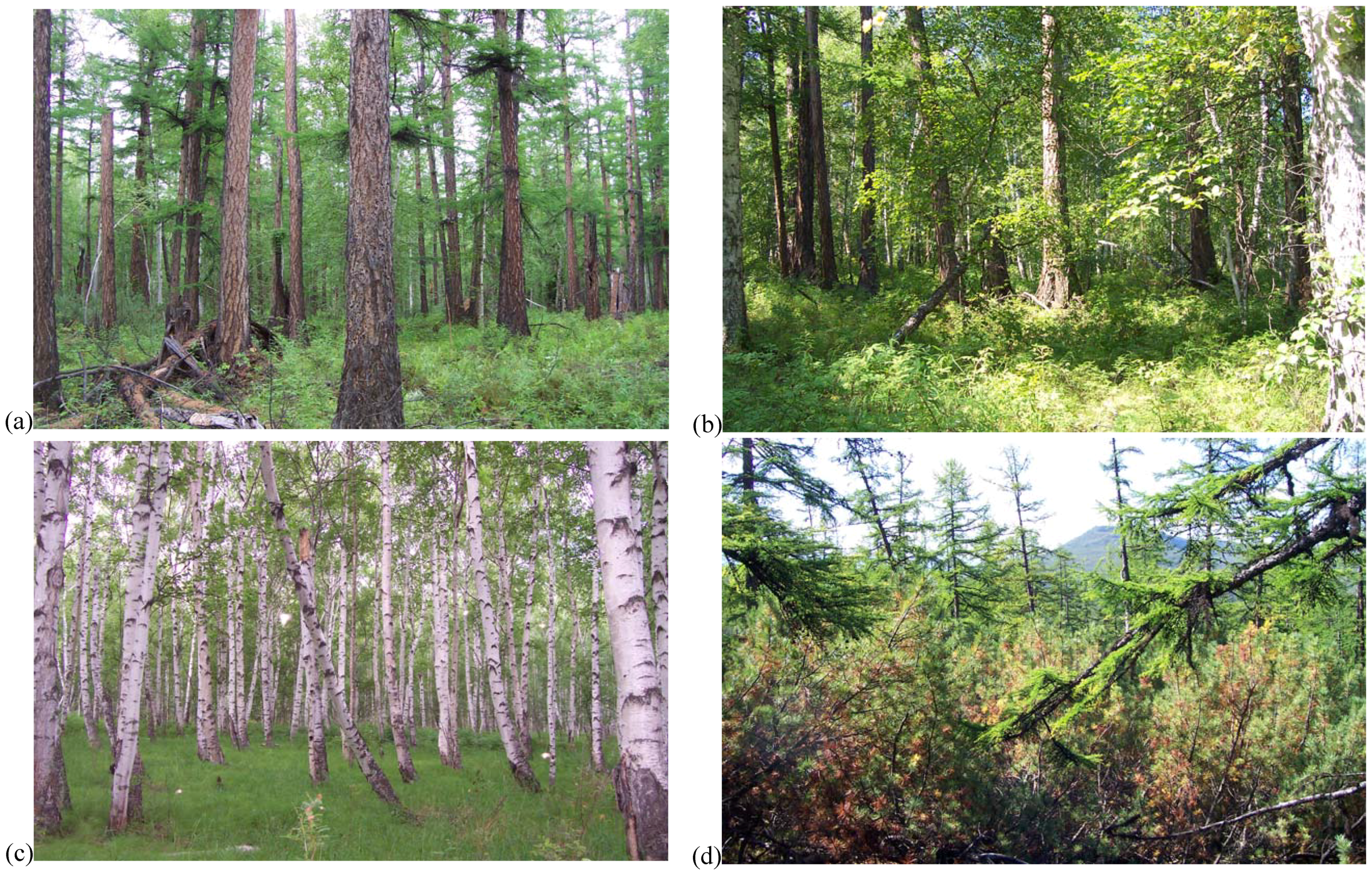
Images of the eight plots are shown in Figure 2. In the lowland plots there is a transition from L. cajanderi-dominated forests (represented by lowland plot 1) to an increasing proportion of B. platyphylla as altitude declines towards the Kamchatka river (lowland plot 2). The same transition is seen in the upland plots, with the upper slopes dominated by L. cajanderi (upland plots 1 and 2) and becoming increasingly mixed with declining altitude (upland plot 3). In the Canadian boreal forest similar transitions have been attributed to clines in moisture and nutrient availability, which increase down-slope [36]. Lowland plot 3 is dominated by B. platyphylla, though this is likely to be a relatively young stand formed following inundation [37].

Mixed forests of L. cajanderi and B. platyphylla extended over all areas observed in the lowlands. This differs from previous accounts which attribute forests in this region to a ‘conifer island’ dominated by Picea ajanensis [4,6,38], though in fact such forests occur only in isolated patches. Russian sources typically overstate the importance of Picea, reflecting its predominant role as a timber tree. Krestov [4] considers Larix-Betula forests to be a secondary replacement of P. ajanensis stands following fire or logging, though there are three reasons why this may not be the case: (a) historical records in Esso from the last century (including numerous photographs) document only forests of Larix in this region, and the name Esso itself derives from the indigenous name for Larix, (b) regenerating Picea were never observed beneath the canopy, and (c) remnant fragments of Picea forest or stumps might have been expected to persist, yet are entirely absent. While Larix-Betula forests may be secondary within the range of P. ajanensis elsewhere (e.g., Sikhote-Alin), in this region they appear to dominate naturally. Such forests are more akin to the ‘light taiga’ forests of Eurasia than the Picea-dominated ‘dark taiga’ found throughout continental Far East Russia. The principal difference in dynamics is that Larix tolerates periodic ground fires, whereas the dark taiga forest is highly sensitive to fire disturbance [14] and destructive insect outbreaks [39]. Intermittent fires allow light-demanding species to persist without competitive exclusion [12].

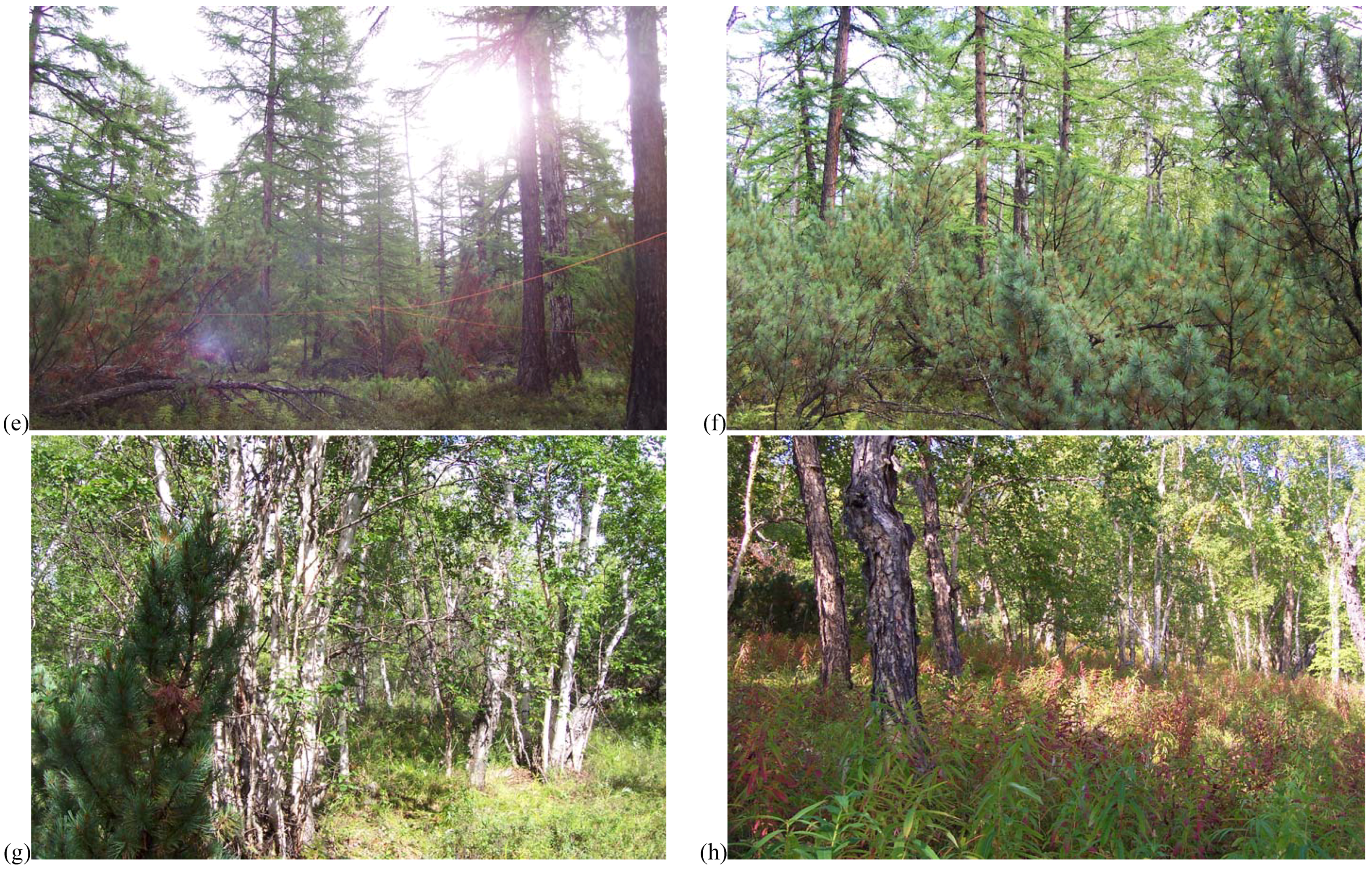
Figure 2. Photographs of forest plots, presented in same sequence as Table 1. (a,b) Lowland mixed Larix cajanderi – Betula platyphylla, (c) lowland B. platyphylla, (d,e) upland L. cajanderi with Pinus pumila sub-canopy, (f) upland mixed L. cajanderi – B. platyphylla, (g) upland B. platyphylla, (h) upland B. ermanii.

Figure 2. Photographs of forest plots, presented in same sequence as Table 1. (a,b) Lowland mixed Larix cajanderi – Betula platyphylla, (c) lowland B. platyphylla, (d,e) upland L. cajanderi with Pinus pumila sub-canopy, (f) upland mixed L. cajanderi – B. platyphylla, (g) upland B. platyphylla, (h) upland B. ermanii.

A debate exists over whether patterns in the distribution of boreal forest types arise from environmental variation, especially topographic [36], or disturbance, or an interaction between the two. Though Betula forms the first canopy in post-fire stands, conifers also regenerate immediately [14,40], with subsequent dynamics driven by mortality, and mixed stands commonly form immediately following disturbance [11,41,42], in line with the initial floristics model of succession [43]. Nevertheless, dispersal limitation may impede some species in reaching certain areas, especially Picea spp. [44]. Though some authors have suggested that Betula spp. often facilitate the regeneration of coniferous species [45], Larix spp. are typically unable to regenerate under a tree overstorey due to shade intolerance and therefore require fire to establish [4]. In general Larix and Betula are unusual amongst temperate tree genera in that the majority of species are tolerant of neither shade nor drought nor water-logging [46], though notable exceptions exist.

Betula ermanii forests form a belt around 600–800 m in the central mountains [6], as seen in upland plot 5, though they cannot form on permafrost or wetlands. The B. ermanii forests are represented by only one plot in the present study, but stands across the whole peninsula are remarkably homogeneous in structure and composition [47]. The tree branches have a characteristic tendency to break at around 1.5 m height due to winter snow-loading [2]. Their replacement at a similar altitude by B. platyphylla (upland plot 4), whose seedlings are better at tolerating wet sites [48], may suggest that this is a water-logged area, which would be supported by the local abundance of Salix bebbiana Sarg. The separation of B. ermanii at high elevations and B. platyphylla at lower is thought to occur because B. ermanii has poor tolerance of hot summer temperatures [49] but is capable of withstanding the lower temperatures characteristic of montane environments, including rapid chills and burial in snow [50,51], perhaps due to its greater investment in roots [48]. By contrast B. platyphylla is more strongly competitive and has a wider range of tolerances [48], though growth rings indicate limitation by low summer temperatures above 300–350 m [21].

3.1. Composition and Structure

The composition, stem density and basal area for all live trees present in the eight plots are summarised in Table 2. Total basal area was consistently greater in the lowland plots (30.3–38.1 m²/ha) than the uplands (7.8–17.0 m²/ha), despite a negligible difference in stem density (upland 191–1,024 stems/ha; lowland 720–872 stems/ha). The greater range of values in the upland plots reflects the wider altitudinal and geographic range which they encompass.

Total basal areas and stem densities fall within the range of values obtained from North American and European forests [12], but there are only two known comparable studies in the region. A 1 ha plot established by Koichi et al. [52] in a regenerating Picea-Betula stand contained 1,071 stems/ha and a basal area of 25.8 m²/ha, enumerated for all stems above 2 cm dbh. Stem density was therefore higher, and basal area lower, than found in our plots, and the composition in terms of coniferous and deciduous stems more even; P. ajanensis dominated (555 stems, 13.27 m²) while B. platyphylla had almost equivalent density and basal area (461 stems, 10.82 m²) and P. tremula formed only a minor component (38 stems, 1.71 m²). By contrast, Dolezal et al. [16] established a 0.4 ha plot in a regenerating post-fire mixed Betula-Larix stand closer in composition to our own and between our two study areas. This had a high density of B. platyphylla (2,583 stems/ha, 17.15 m²/ha) but the regenerating cohort of L. cajanderi remained much smaller (540 stems/ha, 3.13 m²/ha).

Table 2. Structure of old-growth forest plots in Central Kamchatka. Density, basal area (BA) and importance value (IV) for all stems >1 cm dbh corrected to 1 ha for comparative purposes. Numbers of individuals are given to the nearest integer. Pt = Populus tremula, Sc = Salix caprea L., Be = Betula ermanii.

Location	Plot	Betula platyphylla			Larix cajanderi			Other species
		Density	BA	IV	Density	BA	IV	Species	Density	BA	IV
		(stems/ha)	(m2/ha)		(stems/ha)	(m2/ha)			(stems/ha)	(m2/ha)
Lowland	1	320	2.92	26.3	300	31.96	65.6	Pt	100	0.80	8.07
	2	688	13.08	61.3	92	25.00	38.7
	3	864	29.24	97.7	4	1.10	2.04	Sc	4	<0.01	0.23
Upland	1	37	0.27	10.8	147	10.95	87.1	Sc	7	0.06	2.03
	2	68	0.76	12.9	252	15.91	87.1
	3	253	2.51	38.0	140	14.47	59.5	Sc	20	0.03	2.52
	4	764	6.88	81.4	-	Absent	-	Sc	260	0.92	18.6
	5	-	Absent	-	-	Absent	-	Be *	504	16.94	100

*S. caprea is also present within this forest type but absent within the plot.

Table 2. Structure of old-growth forest plots in Central Kamchatka. Density, basal area (BA) and importance value (IV) for all stems >1 cm dbh corrected to 1 ha for comparative purposes. Numbers of individuals are given to the nearest integer. Pt = Populus tremula, Sc = Salix caprea L., Be = Betula ermanii.

Location	Plot	Betula platyphylla			Larix cajanderi			Other species
		Density	BA	IV	Density	BA	IV	Species	Density	BA	IV
		(stems/ha)	(m2/ha)		(stems/ha)	(m2/ha)			(stems/ha)	(m2/ha)
Lowland	1	320	2.92	26.3	300	31.96	65.6	Pt	100	0.80	8.07
	2	688	13.08	61.3	92	25.00	38.7
	3	864	29.24	97.7	4	1.10	2.04	Sc	4	<0.01	0.23
Upland	1	37	0.27	10.8	147	10.95	87.1	Sc	7	0.06	2.03
	2	68	0.76	12.9	252	15.91	87.1
	3	253	2.51	38.0	140	14.47	59.5	Sc	20	0.03	2.52
	4	764	6.88	81.4	-	Absent	-	Sc	260	0.92	18.6
	5	-	Absent	-	-	Absent	-	Be *	504	16.94	100

*S. caprea is also present within this forest type but absent within the plot.

Additional data were collected on the abundance of standing dead wood (Table 3), the relative abundance of which can act as an indicator of old-growth forests [12]. In montane sites the proportion of total stand basal area composed of dead wood varied between 6.3–24.3%, comparable to lowland plots 1 and 2 where the figures were 31.2% and 21.8% respectively. Lowland plot 3 is unusual in this regard as it is likely to be a young stand [37] and therefore contains little dead wood (2.45% of total basal area). The number and size of dead trees was high in some lowland plots, consistent with the pattern in old-growth forests for greater mortality of stems in large size classes than can be accounted for by competitive thinning [53,54].

Table 3. Standing dead wood within old-growth forest plots in Central Kamchatka. Density, basal area (BA) and percentage of the total plot basal area which is dead for all stems >1 cm dbh corrected to 1 ha. Numbers of individuals are given to the nearest integer. Pt = Populus tremula, Sc = Salix caprea, Sb = S. bebbiana, Be = Betula ermanii.

Location	Plot	Betula platyphylla			Larix cajanderi			Other species
		Density	BA	% total BA	Density	BA	% total BA	Species	Density	BA	% total BA
		(stems/ha)	(m2/ha)		(stems/ha)	(m2/ha)			(stems/ha)	(m2/ha)
Lowland	1	16	0.32	0.91	76	15.5	30.7	Pt	76	0.04	0.11
	2	32	0.76	1.96	36	9.84	20.5
	3	52	0.75	2.42	0	0.00	0.00	Sc	4	<0.01	0.03
Upland	1	20	0.32	2.76	7	0.38	3.29	Sc	3	0.05	0.44
	2	16	0.40	2.32	20	2.43	12.7
	3	23	0.72	4.05	10	0.67	3.8	Sc	3	<0.01	0.06
	4	60	1.48	16.0	-	Absent	-	Sb	24	0.28	3.46
	5	-	Absent	-	-	Absent	-	Be	64	5.44	24.3

Table 3. Standing dead wood within old-growth forest plots in Central Kamchatka. Density, basal area (BA) and percentage of the total plot basal area which is dead for all stems >1 cm dbh corrected to 1 ha. Numbers of individuals are given to the nearest integer. Pt = Populus tremula, Sc = Salix caprea, Sb = S. bebbiana, Be = Betula ermanii.

Location	Plot	Betula platyphylla			Larix cajanderi			Other species
		Density	BA	% total BA	Density	BA	% total BA	Species	Density	BA	% total BA
		(stems/ha)	(m2/ha)		(stems/ha)	(m2/ha)			(stems/ha)	(m2/ha)
Lowland	1	16	0.32	0.91	76	15.5	30.7	Pt	76	0.04	0.11
	2	32	0.76	1.96	36	9.84	20.5
	3	52	0.75	2.42	0	0.00	0.00	Sc	4	<0.01	0.03
Upland	1	20	0.32	2.76	7	0.38	3.29	Sc	3	0.05	0.44
	2	16	0.40	2.32	20	2.43	12.7
	3	23	0.72	4.05	10	0.67	3.8	Sc	3	<0.01	0.06
	4	60	1.48	16.0	-	Absent	-	Sb	24	0.28	3.46
	5	-	Absent	-	-	Absent	-	Be	64	5.44	24.3

In numerical terms, in the montane plots between 7.6–13.6% of all standing trunks (excluding snags) were dead, while for lowland plots 1 and 2 the figures were 18.9% and 8.0% respectively. Once again the young cohort of B. platyphylla in lowland plot 3 contained a relatively lower proportion of dead stems (6.0%). By comparison, in European old-growth boreal forests around 10% of standing trunks (including snags) are dead, a figure which appears to be independent of whole-stand basal area [55]. This corresponds well with the Kamchatkan figures.

The quantities of other dead woody matter are shown in Table 4. The high numbers of stumps indicate that competitive thinning has taken place within these plots as the canopies have closed. The ratio of stumps and fallen trunks to standing dead trees is high in B. platyphylla, indicating a tendency for dead stems to fall quickly but decay slowly, a consequence of the slow decomposition of their bark, which also makes them a poor substrate for colonisation [56,57]. In contract, L. cajanderi stems tend to remain standing for prolonged periods before shattering first into snags and only later becoming stumps, as is common for coniferous species [27]. Intriguingly B. ermanii stems also appear to remain standing when dead, likely due to the high density and strength of their wood [2].

Table 4. Dead wood within old-growth forest plots in Central Kamchatka (numbers/ha). Tips are included in brackets with stumps. Snags are defined as dead trees with stems broken above 1.3. Trunks are identifiable fallen trees >5 cm dbh on the forest floor. Pt = Populus tremula, Sc = Salix caprea, Be = Betula ermanii.

Location	Plot	Betula platyphylla			Larix cajanderi			Other species
		Stumps	Snags	Trunks	Stumps	Snags	Trunks	Species	Stumps	Snags	Trunks
Lowland	1	48	0	44	48	44	108	Pt	20	0	0
	2	100 (8)	8	32	20	12	44
	3	200	4	96	0	0	0	Sc	4	0	0
Upland	1	3	0	7	3	0	27	Sc	0	0	0
	2	16	0	16	16 (24)	12	44
	3	47	7	7	3	0	3	Sc	0	0	0
	4	140	12	28				Sc	4	0	0
	5							Be	16	0	16

Table 4. Dead wood within old-growth forest plots in Central Kamchatka (numbers/ha). Tips are included in brackets with stumps. Snags are defined as dead trees with stems broken above 1.3. Trunks are identifiable fallen trees >5 cm dbh on the forest floor. Pt = Populus tremula, Sc = Salix caprea, Be = Betula ermanii.

Location	Plot	Betula platyphylla			Larix cajanderi			Other species
		Stumps	Snags	Trunks	Stumps	Snags	Trunks	Species	Stumps	Snags	Trunks
Lowland	1	48	0	44	48	44	108	Pt	20	0	0
	2	100 (8)	8	32	20	12	44
	3	200	4	96	0	0	0	Sc	4	0	0
Upland	1	3	0	7	3	0	27	Sc	0	0	0
	2	16	0	16	16 (24)	12	44
	3	47	7	7	3	0	3	Sc	0	0	0
	4	140	12	28				Sc	4	0	0
	5							Be	16	0	16

In assessing the abundance of juvenile trees (Table 5), it is immediately apparent that the two Betula species are recruiting readily, likely due to their ability to generate clonal ramets [28,58]. The same applies to P. tremula and S. caprea where they occur. This may be responsible for the maintenance of these species within closed forests, whereas the similarly light-demanding L. cajanderi is unable to recruit from seed in the shade [4]. Sprouting can be a major contributor to regeneration, though is often ignored in favour of explanations based on seed dispersal. In forests of North Carolina, USA, sprouts were found to comprise up to 87% of early regeneration in gaps, and to grow around three times faster than pre-existing saplings [59]. B. platyphylla, being small-seeded, does not tolerate litter and germinating seeds establish best on mineral soil in canopy gaps [60]. In Central Kamchatka it can be seen to colonise recently-burnt areas in very large numbers, whereas in closed forest it regenerates largely through sprouts [58, and pers. obs.]. Locally P. tremula is the only species capable of invading large gaps and recruiting through root suckers [58]. Observed densities of juvenile trees were low in comparison with old-growth boreal forests elsewhere, for example a Canadian study found an average of 1,473 seedlings/ha [61]. This reflects the relative shade-intolerance of Larix and Betula.

Table 5. Juvenile trees within old-growth forest plots in Central Kamchatka (numbers/ha). Dominant tree species are determined on the basis of importance values exceeding 20 (see Table 3); Lc = Larix cajanderi, Bp = Betula platyphylla, Sc = Salix caprea, Be = Betula ermanii, Pt = Populus tremula.

Location	Plot	Dominants	Bp	Lc	Sc	Be	Pt
Lowland	1	Lc/Bp	148	0			84
	2	Bp/Lc	624	0
	3	Bp	72	0	0
Upland	1	Lc	10	0	0
	2	Lc	4	4
	3	Bp/Lc	147	3	73
	4	Bp	384		152
	5	Be			8	224

Table 5. Juvenile trees within old-growth forest plots in Central Kamchatka (numbers/ha). Dominant tree species are determined on the basis of importance values exceeding 20 (see Table 3); Lc = Larix cajanderi, Bp = Betula platyphylla, Sc = Salix caprea, Be = Betula ermanii, Pt = Populus tremula.

Location	Plot	Dominants	Bp	Lc	Sc	Be	Pt
Lowland	1	Lc/Bp	148	0			84
	2	Bp/Lc	624	0
	3	Bp	72	0	0
Upland	1	Lc	10	0	0
	2	Lc	4	4
	3	Bp/Lc	147	3	73
	4	Bp	384		152
	5	Be			8	224

3.2. Stem Heights and Size Distribution

Substantial differences in height between species of trees and locations are evident (Table 6). A mixed-effects analysis taking the ten tallest measured trees from each plot and a random plot effect found significant differences in height among species (Δd = 180.5, d.f. = 4, P < 0.001) due to a greater average height of L. cajanderi and a reduced height of P. tremula and S. caprea relative to Betula spp. Maximum recorded heights achieved by each species were L. cajanderi 31.50 m, B. platyphylla 29.25 m, P. tremula 21.75 m, B. ermanii 18.75 m and S. caprea 5.50 m. A further mixed-effects analysis compared only B. platyphylla and L. cajanderi between upland and lowland plots. This confirmed the significantly greater height of L. cajanderi (Δd = 155.1, d.f. = 1, P < 0.001), and that both species grew taller in lowland plots (Δd = 12.1, d.f. = 1, P < 0.001) with no significant interaction between species and location (Δd = 0.035, d.f. = 1, P = 0.853) indicating that both respond in the same way to lowland conditions. Indeed, the tallest trees of both species occurred in lowland plots, with neither species exceeding 24 m in upland plots.

Table 6. Height and diameter at breast height (dbh) of live trees in old-growth forest plots in Central Kamchatka. Means ± SE except where only a single stem was available. Sc = Salix caprea, Be = Betula ermanii, Pt = Populus tremula.

Location	Plot	Betula platyphylla		Larix cajanderi		Other Species
		Height (m)	dbh (cm)	Height (m)	dbh (cm)	Species	Height (m)	dbh (cm)
Lowland	1	9.32 ± 1.12	8.21 ± 0.77	21.34 ± 1.39	33.99 ± 1.65	Pt	12.08 ± 1.97	8.48 ± 1.13
	2	11.40 ± 1.34	12.01 ± 0.75	24.73 ± 1.16	56.31 ± 3.61
	3	15.00 ± 1.17	18.99 ± 0.57	24	59.1	Sc	Unmeasured	2.2
Upland	1	6.55 ± 0.63	8.70 ± 1.25	14.5 ± 0.51	27.1 ± 1.22	Sc	4.75 ± 0.75	8.05 ± 4.65
	2	7.80 ± 1.45	9.78 ± 1.69	15.21 ± 0.94	26.13 ± 1.40
	3	9.18 ± 1.03	8.88 ± 0.79	17.50 ± 0.78	33.64 ± 2.12	Sc	4.33 ± 0.68	4.21 ± 0.73
	4	8.30 ± 0.59	8.17 ± 0.47	-	-	Sc	3.91± 0.32	4.78 ± 0.37
	5	-	-	-	-	Be	10.4 ± 0.97	15.8 ± 1.18

Table 6. Height and diameter at breast height (dbh) of live trees in old-growth forest plots in Central Kamchatka. Means ± SE except where only a single stem was available. Sc = Salix caprea, Be = Betula ermanii, Pt = Populus tremula.

Location	Plot	Betula platyphylla		Larix cajanderi		Other Species
		Height (m)	dbh (cm)	Height (m)	dbh (cm)	Species	Height (m)	dbh (cm)
Lowland	1	9.32 ± 1.12	8.21 ± 0.77	21.34 ± 1.39	33.99 ± 1.65	Pt	12.08 ± 1.97	8.48 ± 1.13
	2	11.40 ± 1.34	12.01 ± 0.75	24.73 ± 1.16	56.31 ± 3.61
	3	15.00 ± 1.17	18.99 ± 0.57	24	59.1	Sc	Unmeasured	2.2
Upland	1	6.55 ± 0.63	8.70 ± 1.25	14.5 ± 0.51	27.1 ± 1.22	Sc	4.75 ± 0.75	8.05 ± 4.65
	2	7.80 ± 1.45	9.78 ± 1.69	15.21 ± 0.94	26.13 ± 1.40
	3	9.18 ± 1.03	8.88 ± 0.79	17.50 ± 0.78	33.64 ± 2.12	Sc	4.33 ± 0.68	4.21 ± 0.73
	4	8.30 ± 0.59	8.17 ± 0.47	-	-	Sc	3.91± 0.32	4.78 ± 0.37
	5	-	-	-	-	Be	10.4 ± 0.97	15.8 ± 1.18

Tree diameter analyses showed a qualitatively identical pattern to those of height. Diameter is a weak indicator of tree age [62,63], even if the relationship improves in old-growth stands [63]. Previous studies have recorded maximum ages from tree cores for B. ermanii of 180–241 years and B. platyphylla 161–167 years [21], while Krestov [4] believes that B. ermanii and L. cajanderi can exceed 500 years.

Stem size distributions, as described by the Gini co-efficient, were more even for L. cajanderi than B. platyphylla (ANOVA F_1,8 = 12.6, P = 0.007; Table 7), though there was no overall difference between upland and lowland (F_1,8 = 0.001, P = 0.973) or the interaction between species and location (F_1,8 = 0.09, P = 0.776). Statistical results were qualitatively identical for both CV and skewness statistics. This is likely the result of the difference in growth between the two species. L. cajanderi stands tend to form as a single cohort of stems which are thence competitively thinned but remain of approximately equal size. In contrast, B. platyphylla produces new stems from the root collar [58]. If these are continuously produced throughout stand development then a greater size inequality is inevitable. Analysis of the parameters of fitted Weibull distributions revealed a trend towards greater scale parameters in upland plots (F_1,8 = 5.28, P = 0.051), suggesting that these were at a relatively later stage of stand development, despite their shorter stature. Parameters were much greater in L. cajanderi than B. platyphylla for both scale (F_1,8 = 39.0, P < 0.001) and shape (F_1,8 = 31.4, P < 0.001), indicating that these cohorts were at a later stage of maturity.

Table 7. Stem size inequality and distribution within old-growth forest plots in Central Kamchatka: Gini co-efficient (Gini), co-efficient of variation (CV), skewness and scale (b) and shape (c) parameters (means ± SE) of a three-parameter Weibull distribution fit by maximum likelihood. Be = Betula ermanii, Bp = B. platyphylla, Lc = Larix cajanderi, Pt = Populus tremula, Sc = Salix caprea, Sb = S. bebbiana.

Species	Location	Plot	Gini	CV	Skewness	scale (b)	shape (c)
Be	Upland	5	0.45	83.9	1.33	15.0 ± 1.43	1.02 ± 0.09
Bp	Lowland	1	0.44	83.4	1.18	7.22 ± 0.77	1.00 a
Bp	Lowland	2	0.45	81.8	0.95	10.6 ± 0.90	0.93 ± 0.05
Bp	Lowland	3	0.25	44.2	0.09	21.3 ± 0.89	2.36 ± 0.17
Bp	Upland	1	0.25	47.5	−0.05	3.74 ± 1.94	0.60 ± 0.15
Bp	Upland	2	0.37	71.4	0.93	8.18 ± 7.00	1.06 ± 1.92
Bp	Upland	3	0.42	77.9	0.94	8.02 ± 0.97	1.04 ± 0.12
Bp	Upland	4	0.44	80.2	0.96	7.05 ± 0.55	0.96 ± 0.05
Lc	Lowland	1	0.23	40.6	−0.23	36.1 ± 2.33	2.63 ± 0.32
Lc	Lowland	2	0.16	30.7	−0.03	62.3 ± 22.8	3.66 ± 1.56
Lc	Upland	1	0.17	29.8	−0.12	28.6 ± 11.6	3.68 ± 1.74
Lc	Upland	2	0.24	42.4	0.15	29.4 ± 3.46	2.55 ± 0.42
Lc	Upland	3	0.23	40.8	−0.19	37.8 ± 5.04	2.71 ± 0.56
Pt	Lowland	1	0.36	66.9	0.93	8.32 ± 1.51	1.34 ± 0.29
Sc	Upland	3	0.20	42.6	0.63	1.59 ± 0.91	0.74 ± 0.23
Sb	Upland	4	0.34	62.2	0.86	3.89 ± 0.46	1.17 ± 0.15

^a Standard errors are intractable for c = 1

Table 7. Stem size inequality and distribution within old-growth forest plots in Central Kamchatka: Gini co-efficient (Gini), co-efficient of variation (CV), skewness and scale (b) and shape (c) parameters (means ± SE) of a three-parameter Weibull distribution fit by maximum likelihood. Be = Betula ermanii, Bp = B. platyphylla, Lc = Larix cajanderi, Pt = Populus tremula, Sc = Salix caprea, Sb = S. bebbiana.

Species	Location	Plot	Gini	CV	Skewness	scale (b)	shape (c)
Be	Upland	5	0.45	83.9	1.33	15.0 ± 1.43	1.02 ± 0.09
Bp	Lowland	1	0.44	83.4	1.18	7.22 ± 0.77	1.00 a
Bp	Lowland	2	0.45	81.8	0.95	10.6 ± 0.90	0.93 ± 0.05
Bp	Lowland	3	0.25	44.2	0.09	21.3 ± 0.89	2.36 ± 0.17
Bp	Upland	1	0.25	47.5	−0.05	3.74 ± 1.94	0.60 ± 0.15
Bp	Upland	2	0.37	71.4	0.93	8.18 ± 7.00	1.06 ± 1.92
Bp	Upland	3	0.42	77.9	0.94	8.02 ± 0.97	1.04 ± 0.12
Bp	Upland	4	0.44	80.2	0.96	7.05 ± 0.55	0.96 ± 0.05
Lc	Lowland	1	0.23	40.6	−0.23	36.1 ± 2.33	2.63 ± 0.32
Lc	Lowland	2	0.16	30.7	−0.03	62.3 ± 22.8	3.66 ± 1.56
Lc	Upland	1	0.17	29.8	−0.12	28.6 ± 11.6	3.68 ± 1.74
Lc	Upland	2	0.24	42.4	0.15	29.4 ± 3.46	2.55 ± 0.42
Lc	Upland	3	0.23	40.8	−0.19	37.8 ± 5.04	2.71 ± 0.56
Pt	Lowland	1	0.36	66.9	0.93	8.32 ± 1.51	1.34 ± 0.29
Sc	Upland	3	0.20	42.6	0.63	1.59 ± 0.91	0.74 ± 0.23
Sb	Upland	4	0.34	62.2	0.86	3.89 ± 0.46	1.17 ± 0.15

^a Standard errors are intractable for c = 1

The observed irregular structure of the measured stands is consistent with similar studies of old-growth boreal forests elsewhere in the world [61], though the use of stem size distributions to signify the maturity of stands is contentious. Some have argued that size distributions are near-normal for the first ca. 120 years of stand age [39], while in New Zealand CV and skewness declined in maturing stands, causing a contradictory transition towards a normal distribution [53]. A declining distribution of stem sizes is often considered a signal of old-growth [27], but selectively-logged stands can have a similar pattern [64], and stands with remarkably different histories often have similar size distributions [65]. In northeast USA, old-growth forests do not converge on a standard diameter distribution but have a high variance in stem size with low densities of live trees [63].

3.3. Subcanopy

In upland forests, a large proportion of each plot was covered by subcanopy Pinus pumila (Table 8 and see Figure 2d-g), and while also present in one lowland plot, bushes there were of low stature and in poor condition. P. pumila is likely to have a pronounced effect on seedling regeneration patterns and through insulation of the soil will maintain permafrost and prevent thawing to below 40 cm depth [26]. In other forests, the woody sub-canopy may influence spatial patterns of regeneration, for example Rhododendron hodgsonii Hook. in Central Bhutan [66]. Here other subcanopy species such as Alnus fruticosa and Salix udensis Trautv. et Mey. colonised sizeable patches but these were scattered and unlikely to have major impacts on seedlings. An exception is where hollows formed due to spring snow melt, and in such places A. fruticosa frequently dominated to the exclusion of all other woody species.

Table 8. Percentage subcanopy cover within old-growth forest plots in Central Kamchatka. Dominant tree species are determined on the basis of importance values exceeding 20 (see Table 2); Lc = Larix cajanderi, Bp = Betula platyphylla, Be = B. ermanii.

Location	Plot	Dominants	Pinus pumila	Alnus fruticosa	Salix caprea	Salix udensis
Lowland	1	Lc/Bp	9.64	-	-	-
	2	Bp/Lc	-	-	-	-
	3	Bp	-	-	-	-
Upland	1	Lc	60.67	1.17	-	-
	2	Lc	50.76	0.20	-	-
	3	Lc/Bp	50.60	3.27	0.17	-
	4	Bp	22.84	-	-	4.12
	5	Be	6.88	-	-	-

Table 8. Percentage subcanopy cover within old-growth forest plots in Central Kamchatka. Dominant tree species are determined on the basis of importance values exceeding 20 (see Table 2); Lc = Larix cajanderi, Bp = Betula platyphylla, Be = B. ermanii.

Location	Plot	Dominants	Pinus pumila	Alnus fruticosa	Salix caprea	Salix udensis
Lowland	1	Lc/Bp	9.64	-	-	-
	2	Bp/Lc	-	-	-	-
	3	Bp	-	-	-	-
Upland	1	Lc	60.67	1.17	-	-
	2	Lc	50.76	0.20	-	-
	3	Lc/Bp	50.60	3.27	0.17	-
	4	Bp	22.84	-	-	4.12
	5	Be	6.88	-	-	-

3.4. Soils

Soil characteristics varied considerably among plots (Table 9). There were relatively few differences overall between the locations, apart from greater C content in upland soils (∆d = 376.3, df = 1, P < 0.001) and a tendency towards lower pH in upland plots (∆d = 3.38, df = 1, P = 0.066). Otherwise there were no significant differences in content of NO_x, NH_y, phosphate, total P, total N or total S (P > 0.05 for all comparisons). Differences among individual plots were more pronounced, with variation in their content of NO_x (F_7,39 = 2.39, P = 0.039), NH_y (F_7,40 = 2.74, P = 0.020), phosphate (F_7,38 = 8.54, P < 0.001), total C (F_7,40 = 3.40, P = 0.006), total N (F_7,40 = 7.41, P < 0.001), total S (F_7,40 = 11.42, P < 0.001) and pH (F_7,40 = 5.25, P < 0.001), though not total P (F_7,40 = 1.38, P = 0.241). The higher C content of upland soils may be the result of lower temperatures and consequently a slower decomposition rate. Otherwise it is notable that soils from the plots dominated by birch (B. ermanii or B. platyphylla) had higher NO_x and elemental S, while little N or S was present in plots containing L. cajanderi.

Table 9. Soil characteristics of old-growth forest plots in Central Kamchatka, means ± SE. Superscript letters denote significant differences between plots where detected (Tukey’s HSD; see text for details).

Location	Plot	NOx	NHy	PO43+	Total P	Total C	Total N	Total S	pH
		(mg/kg)	(mg/kg)	(mg/kg)	(mg/kg)	(g/kg)	(g/kg)	(g/kg)
Lowland	1	18.0 ± 9.80	7.17 ± 0.30 ab	3.69 ± 0.68 a	849 ± 80	63.1 ± 6.3 ab	2.45 ± 0.28 b	0.24 ± 0.05 c	6.40 ± 0.16 a
	2	15.8 ± 5.22	12.6 ± 4.12 ab	1.42 ± 0.42 ab	669 ± 66	92.2 ± 7.0 ab	3.78 ± 0.23 ab	0.43 ± 0.01 bc	5.72 ± 0.14 bc
	3	68.2 ± 34.9	29.9 ± 9.16 a	0.59 ± 0.13 bc	600 ± 90	119 ± 9.5 ab	6.38 ± 0.65 a	1.19 ± 0.23 a	5.89 ± 0.21 abc
Upland	1	9.08 ± 3.38	25.4 ± 13.5 ab	0.56 ± 0.31 bc	593 ± 118	126 ± 18.7 a	4.45 ± 0.68 ab	0.35 ± 0.03 bc	5.61 ± 0.12 bc
	2	9.46 ± 2.29	4.14 ± 0.99 b	0.69 ± 0.17 bc	747 ± 75	118 ± 24.7 ab	4.26 ± 0.85 ab	0.31 ± 0.10 bc	5.38 ± 0.14 c
	3	16.2 ± 5.85	14.6 ± 6.38 ab	0.33 ± 0.17 c	589 ± 123	48.4 ± 8.4 b	2.04 ± 0.27 b	0.22 ± 0.05 c	6.08 ± 0.14 ab
	4	19.3 ± 6.57	25.2 ± 9.33 ab	0.45 ± 0.14 bc	575 ± 83	130 ± 30.0 a	6.62 ± 1.24 a	0.70 ± 0.07 b	5.65 ± 0.08 bc
	5	43.5 ± 12.2	31.3 ± 5.89 a	0.86 ± 0.09 b	789 ± 67	106 ± 7.1 ab	6.28 ± 0.24 a	0.62 ± 0.02 bc	5.65 ± 0.05 bc

Table 9. Soil characteristics of old-growth forest plots in Central Kamchatka, means ± SE. Superscript letters denote significant differences between plots where detected (Tukey’s HSD; see text for details).

Location	Plot	NOx	NHy	PO43+	Total P	Total C	Total N	Total S	pH
		(mg/kg)	(mg/kg)	(mg/kg)	(mg/kg)	(g/kg)	(g/kg)	(g/kg)
Lowland	1	18.0 ± 9.80	7.17 ± 0.30 ab	3.69 ± 0.68 a	849 ± 80	63.1 ± 6.3 ab	2.45 ± 0.28 b	0.24 ± 0.05 c	6.40 ± 0.16 a
	2	15.8 ± 5.22	12.6 ± 4.12 ab	1.42 ± 0.42 ab	669 ± 66	92.2 ± 7.0 ab	3.78 ± 0.23 ab	0.43 ± 0.01 bc	5.72 ± 0.14 bc
	3	68.2 ± 34.9	29.9 ± 9.16 a	0.59 ± 0.13 bc	600 ± 90	119 ± 9.5 ab	6.38 ± 0.65 a	1.19 ± 0.23 a	5.89 ± 0.21 abc
Upland	1	9.08 ± 3.38	25.4 ± 13.5 ab	0.56 ± 0.31 bc	593 ± 118	126 ± 18.7 a	4.45 ± 0.68 ab	0.35 ± 0.03 bc	5.61 ± 0.12 bc
	2	9.46 ± 2.29	4.14 ± 0.99 b	0.69 ± 0.17 bc	747 ± 75	118 ± 24.7 ab	4.26 ± 0.85 ab	0.31 ± 0.10 bc	5.38 ± 0.14 c
	3	16.2 ± 5.85	14.6 ± 6.38 ab	0.33 ± 0.17 c	589 ± 123	48.4 ± 8.4 b	2.04 ± 0.27 b	0.22 ± 0.05 c	6.08 ± 0.14 ab
	4	19.3 ± 6.57	25.2 ± 9.33 ab	0.45 ± 0.14 bc	575 ± 83	130 ± 30.0 a	6.62 ± 1.24 a	0.70 ± 0.07 b	5.65 ± 0.08 bc
	5	43.5 ± 12.2	31.3 ± 5.89 a	0.86 ± 0.09 b	789 ± 67	106 ± 7.1 ab	6.28 ± 0.24 a	0.62 ± 0.02 bc	5.65 ± 0.05 bc

3.5. Comparisons with Other Boreal Forests

The most obvious analogues of Kamchatkan forests are the well-studied forests of central Alaska [11]. During the Tertiary, a circumpolar forest extended across the major landmasses of the northern hemisphere. This was split by the formation of the Bering Straits approximately 5.32 Ma [17], and although a land bridge was present at glacial maxima during the Quaternary, and the region was only partially glaciated, it is highly unlikely that any floristic interchange between the forest zones occurred. The two regions share approximately a third of their flora, with a further third each being restricted to either side of the Bering Straits [18]. However, shared species tend to be those which are cosmopolitan and cold-adapted, and the two landmasses have entirely different tree floras.

The differences in the forest structures are pronounced (Table 10 and see [67]), and even congeneric tree species differ markedly. L. cajanderi frequently dominates upland forests of Kamchatka, while its sister species in Alaska L. laricina (Du Roi) K. Koch, is by contrast a relatively unimportant tree confined to lowland areas with a reliable groundwater supply and is vulnerable to fire [18]. Unlike the extensive stands of Populus tremuloides Michx. in Alaska, P. tremula in Kamchatka is present only in isolated clonal patches of 200–400 m² which it dominates, with these typically occurring the lower parts of south-facing slopes.

Table 10. Comparison of major forest types in central Kamchatka and central Alaska.

Location	Kamchatka	Alaska
Above tree line	Alnus or P. pumila scrub	Alnus scrub
Montane forests at tree line	B. ermanii	B. neoalaskana Sarg.
North-facing slopes (and other cold areas)	Sparse forest of L. cajanderi underlain by dense thickets of P. pumila.	Picea mariana (Mill.) B.S.P.
Other areas	Mixed and variable forest of L. cajanderi and B. platyphylla, the latter predominating on warm, wet sites and at the base of slopes	Picea glauca (Moench) Voss

Table 10. Comparison of major forest types in central Kamchatka and central Alaska.

Location	Kamchatka	Alaska
Above tree line	Alnus or P. pumila scrub	Alnus scrub
Montane forests at tree line	B. ermanii	B. neoalaskana Sarg.
North-facing slopes (and other cold areas)	Sparse forest of L. cajanderi underlain by dense thickets of P. pumila.	Picea mariana (Mill.) B.S.P.
Other areas	Mixed and variable forest of L. cajanderi and B. platyphylla, the latter predominating on warm, wet sites and at the base of slopes	Picea glauca (Moench) Voss

3.6. Threats and Further Study Required

Given the location of Kamchatka, the low density of human inhabitation, the limited scale of timber extraction and the existence of several IUCN World Heritage Sites, one might presume that threats to its forests are limited. Since L. cajanderi is considered low-quality timber [68], there is unlikely to be commercial exploitation of these forests, though those of Picea ajanensis remain under threat [8]. It is also anticipated that the relative isolation of Kamchatka from the mainland will reduce the spread of invasive species, of which there are remarkably few.

Nevertheless, vigilance is warranted. While the impacts of phytophagous insects are largely unknown, patches of defoliated L. cajanderi are visible from the air in the Central Depression (pers. obs.). In Central Alaska, larch sawfly outbreaks (Pristiphora erichsonii (Hartig)) were first reported in 1993, but have subsequently caused mortality of trees over hundreds of thousands of hectares [69], and Kamchatkan forests may be similarly vulnerable.

A large gap in our knowledge arises due to a lack of information on fire frequency, whether at surface or crown level. In average years only 10–20% of Russian forest fires are thought to be stand-replacing crown fires [70,71], with Larix tolerating occasional ground fire [14]. Evidence from a wide variety of boreal forests suggests fire intervals of at least 25 years and occasionally greater than 200 years [71,72]. Fire intervals in Russian larch forests are thought to be between 90–130 years [71], within the range reported for North American boreal forests [23]. Mean fire intervals can however be misleading as they disguise a high variance, which leads to a wide variety of stand ages at the landscape scale [73], while if burning is prevented, forests can develop into unnatural states [74]. Careful management is therefore required, which is best accomplished by the maintenance of large tracts to permit natural fire cycles on the landscape scale [73]. Kamchatka is one of the few regions in the world where such a management option remains feasible.

Despite the relative continentality and low rainfall of interior Kamchatka, the late snow melt and foggy weather throughout the summer substantially reduce the risk of wildfires [6]. Local opinion, however, is that summers are becoming increasingly hot and clear. Climate change may be expected to increase the frequency of fires [75], though this is difficult to detect. Official Russian fire statistics document a modest increase over recent decades [76], while satellite data instead suggest an almost tenfold increase since the mid-1990s, dramatically greater than in North America [22,23].

At present it is impossible to infer what further impacts climate change may have. In Alaska, large-scale loss of permafrost is anticipated as its temperature is now typically warmer than −2 °C [77]. While only 2.1% of permafrost has been lost in the last 90 years, permafrost temperature has increased by 0.7 °C per decade since 1970, driven by regional warming and changes in the degree of insulation provided by snow and vegetation. If replicated in Kamchatka, this is likely to lead to major alterations in the distribution and composition of plant communities. Without appropriate baseline data this will be impossible to monitor. However, this also presents an opportunity, and Kamchatka could potentially become a globally-important region for assessing the effects of climate change independent of human interactions.