

Algorithms in Tomography and Related Inverse Problems—A Review

Abstract
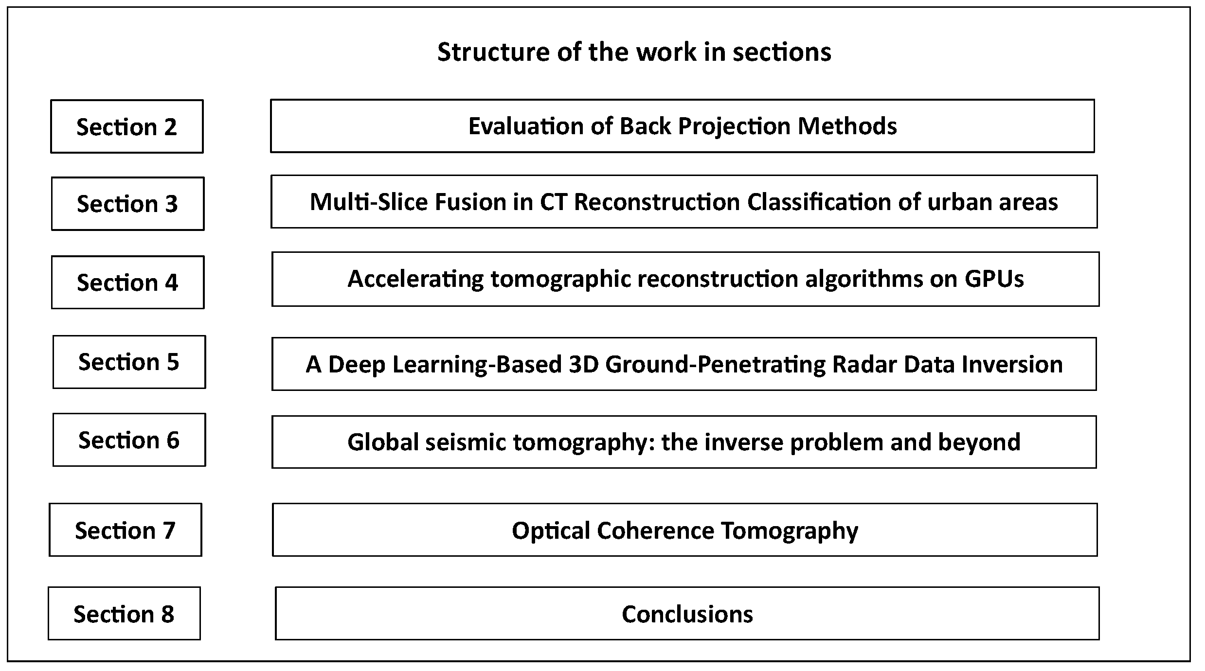
:1. Introduction
1.1. Tomographic Reconstruction Techniques, Principles, and New Approaches
1.2. Special Topics in Tomography
1.3. Tomographic Implementation Algorithms
1.4. Tomographic Imaging: From SAR, Geology, to Medical Advances
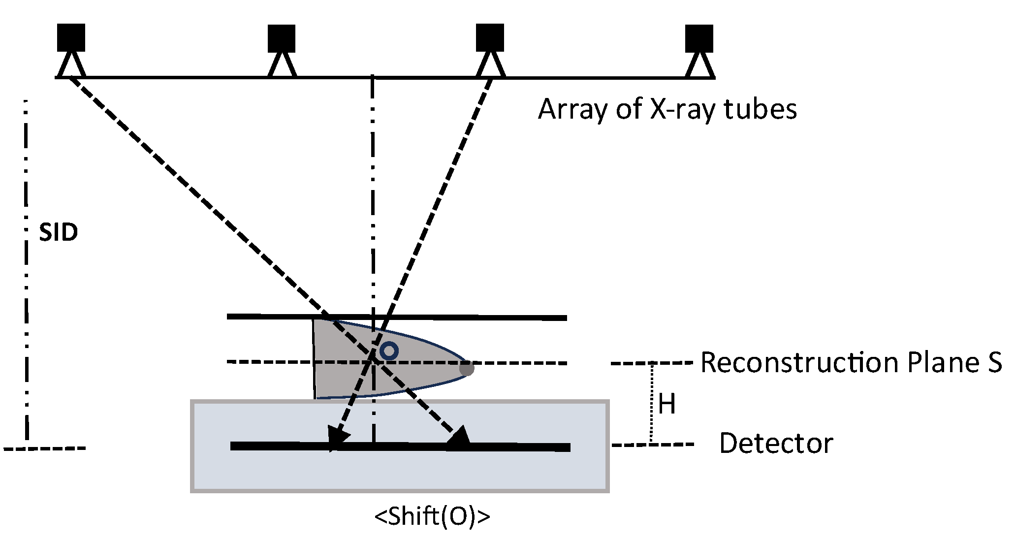
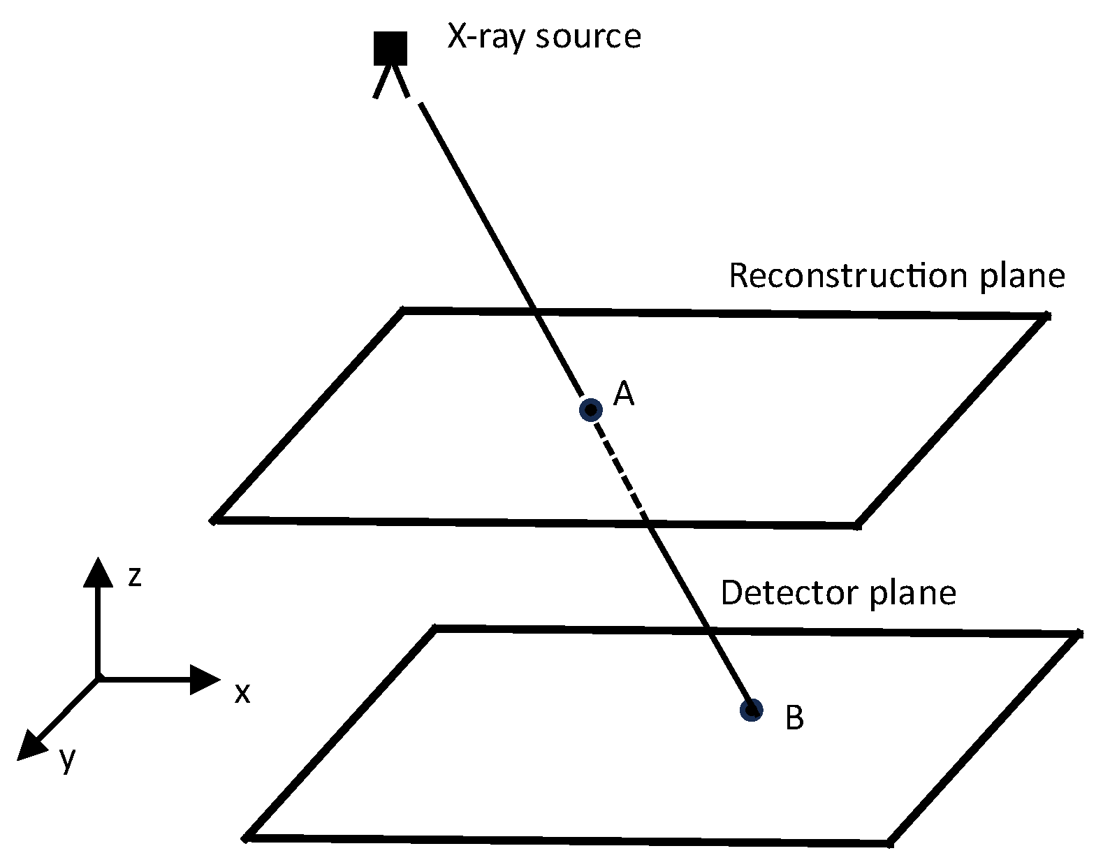
2. Evaluation of Backprojection Methods
- Step 1.
- SAA Tomosynthesis Reconstruction:
- Step 2.
- Point-by-Point Backprojection:
- Step 3.
- Backprojection Variants. α-Trimmed BP Technique:
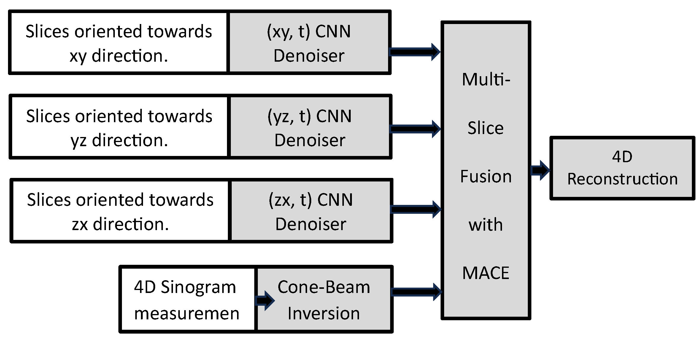
3. Multi-Slice Fusion in CT Reconstruction
- Step 1.
- Formulate the reconstruction problem using the MAP approach:
- Step 2.
- Express the data fidelity term as the sum of squared differences between sinogram measurements and the forward model:
- Step 3.
- Step 4.
- Formulate each as the MAP estimation for a Gaussian denoising problem, where represents a prior model, and is the noise standard deviation.
- Step 5.
- Modify the optimization problem to incorporate different regularizers, resulting in a consensus equilibrium formulation.
- Step 6.
- Define proximal maps and for each term in the optimization problem. Create a stacked operator ) that maps from to , where represents the stacked representative variable:
- Step 7.
- Formulate the consensus equilibrium equation , where is an averaging operator.
- Step 8.
- Derive the fixed-point relationship for the consensus equilibrium solution , which stands as a fixed point within the mapping denoted as .
- Step 9.
- Implement an iterative fixed-point algorithm (e.g., Mann iteration) to compute the equilibrium solution.
- Step 10.
- Use a modified update operator that involves iterative coordinate descent (ICD) for computational efficiency.
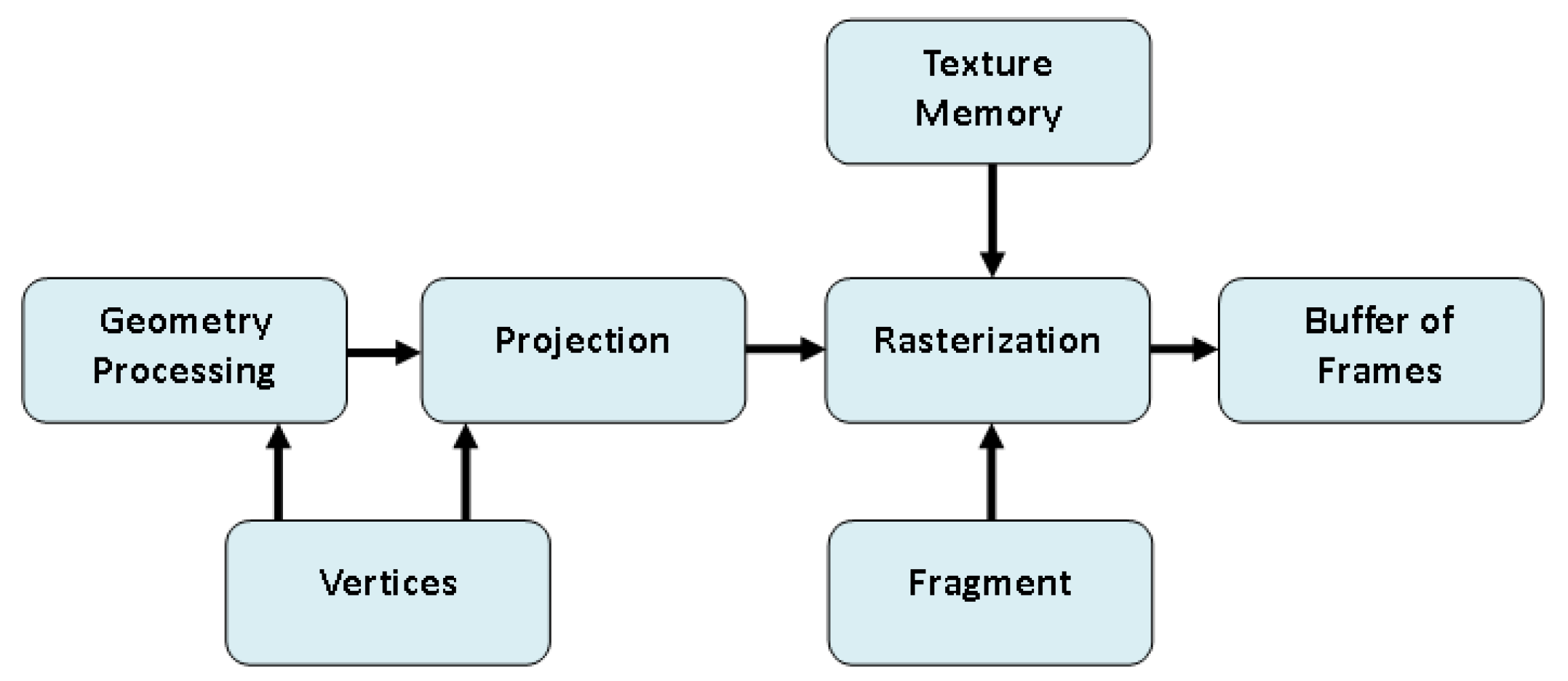
4. Accelerating Popular Tomographic Reconstruction Algorithms on Commodity PC Graphics Hardware
- Step 1.
- Notation and Imaging Modalities:
- A volumetric object is defined by its attenuation function .
- Two imaging modalities are considered: transmission X-ray (external source) and emission X-ray (metabolic sources within the object).
- Mathematical formulations and for recording intensity values on a 2D detector for both modalities are provided.
- Step 2.
- Vector Processing for CT:
- Introduction of vector processing for CT using a standardized notation (, , , , etc.).
- The shift from pixel-centric to voxel-centric representation for transmission X-ray.
- Formulation of voxel-centric representation for emission X-ray.
- Step 3.
- Projection and Backprojection Operators:
- Introduction of projection () and backprojection () operators as matrices.
- Dynamic computation of elements using interpolators integrated into rasterization hardware.
- Step 4.
- Reconstruction Methods:
- Feldkamp algorithmDepth correction factor () during backprojection.Grid update equation expressed in condensed notation.
- SART (Simultaneous Algebraic Reconstruction Technique)Grid update equation for SART involving a relaxation factor ().
- OS-EM (Ordered Subsets Expectation Maximization)Grid update equation for OS-EM algorithm .
5. A Deep Learning-Based 3D Ground-Penetrating Radar Data Inversion
- A dedicated 3D denoising network, referred to as the “Denoiser,” has been meticulously crafted to combat noise interference within GPR C-scans, particularly in the presence of complex and heterogeneous soil environments. This denoiser incorporates a compact 3D convolutional neural network (CNN) architecture, leveraging residual learning principles and a feature attention mechanism to effectively distill the reflection signatures of subsurface objects from noisy C-scans.
- Following the denoising process, a 3D U-shaped encoder-decoder network, aptly named the “Inverter,” is purposefully designed. Its primary function is to translate the denoised C-scans, as predicted by the denoiser, into comprehensive subsurface 3D permittivity maps. To ensure robust feature extraction across a spectrum of objects with diverse properties, the inverter incorporates multi-scale feature aggregation modules.
- To achieve optimal performance, a meticulously devised three-step independent learning strategy is employed, facilitating the pre-training and fine-tuning of both the denoiser and inverter components.
DENOISING, Inverter, and Training
- Initial Feature Extraction:
- An initial feature extraction module is employed, consisting of a 3 × 3 × 3 convolutional layer with channels and 1 × 1 × 1 strides.This module captures the initial features () from the noisy input C-scans ().
- The process involves a 3D convolutional layer ) and a Rectified Linear Unit (ReLU) activation function .
- Feature Learning Modules:
- After initial feature extraction, feature learning modules are applied, each consisting of two residual blocks and one feature attention block.
- Residual blocks utilize identity mapping to address gradient explosion concerns.
- Residual learning is formulated for each block ( and ) and then a feature attention block is introduced to emphasize the significance of features.
- The attention mechanism involves global average pooling to compute channel-wise statistics and a gating mechanism using fully connected layers and a Sigmoid function.
- The attended feature map is generated through channel-wise multiplication and added to the original feature map via a residual connection.
- Reconstruction Module:
- A reconstruction module featuring a one-channel convolutional layer with residual learning is employed.
- This module reconstructs the denoised C-scan () using the learned feature representations.
- 3D U-Net Structure:
- The inverter follows the structure of the 3D U-Net architecture, comprising both an encoder and a decoder with skip connections.
- Multi-Scale Feature Aggregation (MSFA) Mechanism:
- MSFA is introduced within each encoding and decoding block to capture features at various scales effectively.
- Each MSFA module includes three 3 × 3 × 3 convolutional layers with 1 × 1 × 1 strides.
- The increased number of convolutional layers deepens the network, enhancing its nonlinear mapping capabilities and facilitating the extraction of larger-scale features from object reflections.
- Receptive Field (RF) Calculation:
- The RF size of the output feature map generated by the convolutional layer in the MSFA module is calculated using the formula .
- The choice of fixed kernel size ( 3 and 1) leads to different RF sizes, allowing for the capture of multiple scales.
- Multi-Scale Feature Map Combination:
- Feature maps , , and with different RF sizes are combined in the channel dimension within each encoding and decoding block.
- The consolidated multi-scale feature map ) is obtained by concatenating these feature maps.
- Efficient Multi-Scale Feature Capture:
- Unlike approaches that introduce additional parallel convolutional layers, the MSFA module directly integrates feature maps from successive convolutional layers with different receptive fields.
- This design choice aims to efficiently capture multi-scale features from reflection patterns in GPR C-scans influenced by diverse subsurface object properties.
- Overall, the MSFA mechanism is introduced to enhance the network’s ability to represent the nonlinear mapping from C-scans to 3D permittivity maps, taking into account multi-scale features in subsurface imaging.
- Step 1:
- Denoiser Pre-training
- Objective: Train the denoiser component using a diverse dataset of noisy and noise-free C-scans.
- Loss Function: Mean Squared Error (MSE) between the predicted denoised C-scan and the corresponding ground truth ().
- Loss Function Formula:
- Optimizer: Adam optimizer.
- Step 2:
- Inverter Pre-training
- Objective: Pre-train the inverter using noise-free C-scan ground truth () as input data.
- Loss Function: Mean Absolute Error (MAE) between the predicted permittivity map and the ground truth .
- Loss Function Formula:
- Optimizer: Adam optimizer.
- Step 3:
- Fine-tune the Pre-trained Networks (Transfer Learning)
- Additional Data Creation: Generate a small dataset containing new scenarios.
- Initial Network States: Utilize the pre-trained networks as the starting point for fine-tuning.
- Parameter Updates: Further refine the network parameters by minimizing the loss functions and using the new training dataset until convergence.
- Enhanced Networks: After fine-tuning, the networks are better suited to handle a broader range of scenarios.
- Objective: Improve networks’ adaptability and robustness.
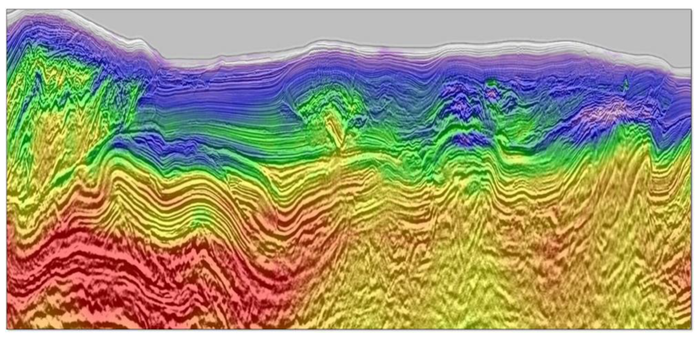
6. Global Seismic Tomography: The Inverse Problem and Beyond
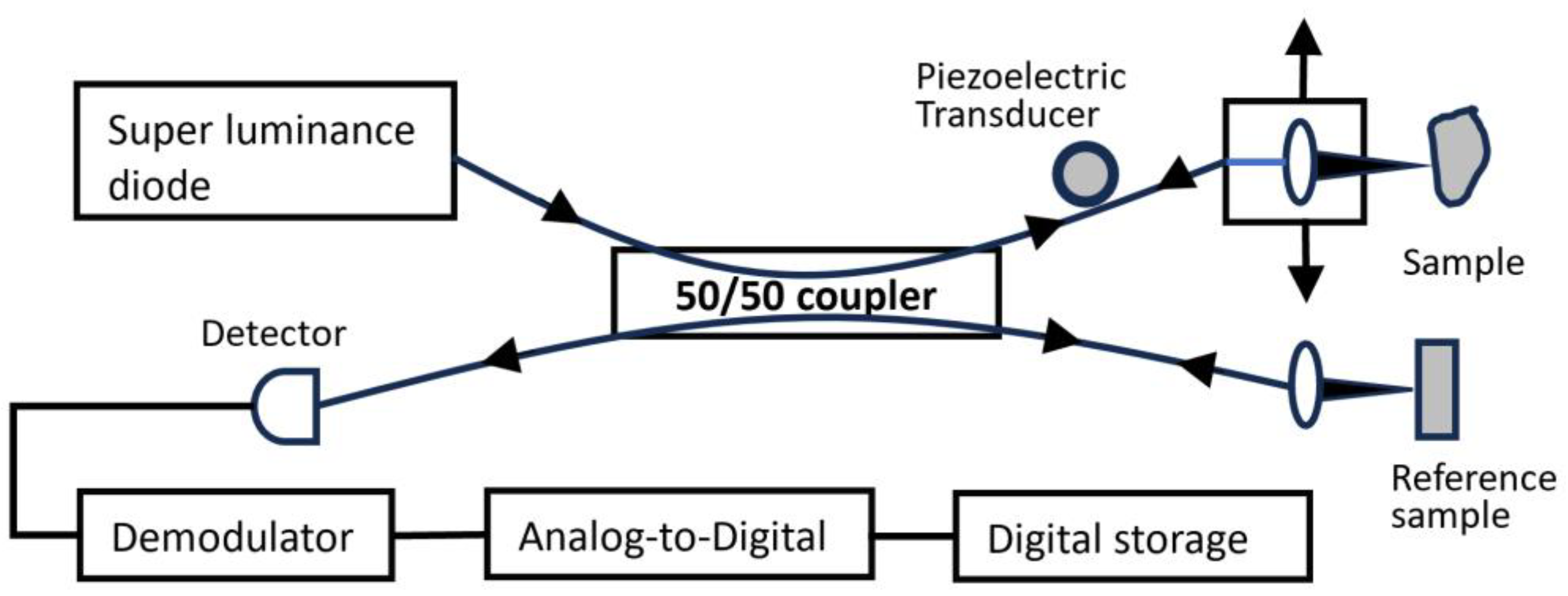
7. Optical Coherence Tomography
- Data Acquisition:
- Light Source: Generates coherent light.
- Interferometer: Splits the light into sample and reference arms.
- Sample Arm: Directs light onto the sample.
- Reference Arm: Sends light to a reference mirror.
- Interference Detection: Combines sample and reference beams; interference is detected.
- Signal Processing:
- Interference Signal Processing: Extracts the interference signal.
- Fourier Transform: Converts the interference signal from time to frequency domain.
- A-Scan Generation: Produces an A-scan (depth profile).
- Image Reconstruction:
- B-Scan Formation: Combines multiple A-scans to form a B-scan (cross-sectional image).
- En-face Image Generation: Constructs en-face images at different depths.
- Image Enhancement and Analysis:
- Speckle Reduction: Techniques to reduce speckle noise.
- Contrast Enhancement: Improves visibility of structures.
- Segmentation: Identifies boundaries and structures in the OCT images.
- 3D Rendering: Creates three-dimensional representations of the imaged volume.
- Image Display and Analysis:
- Visualization: Displays OCT images in real-time.
- Quantitative Analysis: Extracts numerical information from images.
- Clinical Decision Support: Provides support for medical diagnoses.
- Advanced Algorithms:
- Motion Correction: Compensates for motion artifacts.
- Doppler OCT: Measures blood flow within tissues.
- Polarization-Sensitive OCT: Provides additional tissue information based on polarization properties.
- Machine Learning: Incorporates machine learning techniques for image analysis and pattern recognition.
- Data Storage and Management:
- Database: Stores acquired OCT data.
- Archiving: Manages storage of large datasets for future reference.
- Integration with Other Modalities:
- Multimodal Imaging: Integrates OCT with other imaging modalities for comprehensive diagnostics.
- Clinical Applications:
- Ophthalmology: Retinal imaging, anterior segment imaging.
- Dermatology: Skin imaging.
- Cardiology: Cardiovascular imaging.
- Endoscopy: Imaging within body cavities.
- Feedback Loop:
- System Calibration: Ensures accuracy and reliability.
- User Feedback: Allows for adjustments based on user input.
- System Optimization: Continuous improvement based on performance feedback.
8. Conclusions
Author Contributions
Funding
Data Availability Statement
Conflicts of Interest
References
- Gordon, R.; Herman, G.T. Three-Dimensional Reconstruction from Projections: A Review of Algorithms. Int. Rev. Cytol. 1974, 38, 111–151. [Google Scholar] [CrossRef]
- Colsher, J.G. Iterative three-dimensional image reconstruction from tomographic projections. Comput. Graph. Image Process 1977, 6, 513–537. [Google Scholar] [CrossRef]
- Clackdoyle, R.; Defrise, M. Tomographic Reconstruction in the 21st Century. IEEE Signal Process. Mag. 2010, 27, 60–80. [Google Scholar] [CrossRef]
- Hornegger, J.; Maier, A.; Kowarschik, M. CT Image Reconstruction Basics. 2016 [Source: Radiology Key]. Available online: https://radiologykey.com/ct-image-reconstruction-basics/ (accessed on 15 October 2023).
- Khan, U.; Yasin, A.; Abid, M.; Awan, I.S.; Khan, S.A. A Methodological Review of 3D Reconstruction Techniques in Tomographic Imaging. J. Med. Syst. J. Med Syst. 2018, 42, 190. [Google Scholar] [CrossRef]
- Goshtasby, A.; Turner, D.A.; Ackerman, L.V. Matching of tomographic slices for interpolation. IEEE Trans. Med. Imaging 1992, 11, 507–516. [Google Scholar] [CrossRef]
- Fessler, J.A. Statistical Image Reconstruction Methods for Transmission Tomography. In Handbook of Medical Imaging; SPIE Press: Bellingham, WA, USA, 2000; Volume 1, pp. 1–70. [Google Scholar] [CrossRef]
- Yu, D.F.; Fessler, J.A. Edge-preserving tomographic reconstruction with nonlocal regularization. IEEE Trans. Med. Imaging 2002, 21, 159–173. [Google Scholar] [CrossRef] [PubMed]
- Chandra, S.S.; Svalbe, I.D.; Guedon, J.; Kingston, A.M.; Normand, N. Recovering Missing Slices of the Discrete Fourier Transform Using Ghosts. IEEE Trans. Image Process. 2012, 21, 4431–4441. [Google Scholar] [CrossRef] [PubMed]
- Zhou, W.; Lu, J.; Zhou, O.; Chen, Y. Evaluation of Back Projection Methods for Breast Tomosynthesis Image Reconstruction. J. Digit. Imaging 2014, 28, 338–345. [Google Scholar] [CrossRef] [PubMed]
- Chetih, N.; Messali, Z. Tomographic image reconstruction using filtered back projection (FBP) and algebraic reconstruction technique (ART). In Proceedings of the 3rd International CEIT 2015, Tlemcen, Algeria, 25 May 2015. [Google Scholar] [CrossRef]
- Somigliana, A.; Zonca, G.; Loi, G.; Sichirollo, A.E. How Thick Should CT/MR Slices be to Plan Conformal Radiotherapy? A Study on the Accuracy of Three-Dimensional Volume Reconstruction. Tumori J. 1996, 82, 470–472. [Google Scholar] [CrossRef]
- Gourion, D.; Noll, D. The inverse problem of emission tomography. IOP Publ. Inverse Probl. 2002, 18, 1435–1460. [Google Scholar] [CrossRef]
- Petersilka, M.; Bruder, H.; Krauss, B.; Stierstorfer, K.; Flohr, T.G. Technical principles of dual source CT. Eur. J. Radiol. 2008, 68, 362–368. [Google Scholar] [CrossRef]
- Saha, S.K.; Tahtali, M.; Lambert, A.; Pickering, M. CT reconstruction from simultaneous projections: A step towards capturing CT in One Go. Comput. Methods Biomech. Biomed. Eng. Imaging Vis. 2014, 5, 87–99. [Google Scholar] [CrossRef]
- Miqueles, E.; Koshev, N.; Helou, E.S. A Backprojection Slice Theorem for Tomographic Reconstruction. IEEE Trans. Image Process. 2018, 27, 894–906. [Google Scholar] [CrossRef]
- Willemink, M.J.; Noël, P.B. The evolution of image reconstruction for CT—From filtered back projection to artificial intelligence. Eur. Radiol. 2019, 29, 2185–2195. [Google Scholar] [CrossRef] [PubMed]
- Wang, G.; Ye, J.C.; De Man, B. Deep learning for tomographic image reconstruction. Nat. Mach. Intell. 2020, 2, 737–748. [Google Scholar] [CrossRef]
- Jung, H. Basic Physical Principles and Clinical Applications of Computed Tomography. Prog. Med. Phys. 2021, 32, 1–17. [Google Scholar] [CrossRef]
- Withers, P.J.; Bouman, C.; Carmignato, S.; Cnudde, V.; Grimaldi, D.; Hagen, C.K.; Stock, S.R. X-ray computed tomography. Nat. Rev. Dis. Primers 2021, 1, 18. [Google Scholar] [CrossRef]
- Seletci, E.D.; Duliu, O.G. Image Processing and Data Analysis in Computed Tomography. Rom. J. Phys. 2007, 72, 764–774. [Google Scholar]
- Miao, J.; Förster, F.; Levi, O. Equally sloped tomography with oversampling reconstruction. Phys. Rev. B 2005, 72, 052103. [Google Scholar] [CrossRef]
- Whiteley, W.; Luk, W.K.; Gregor, J. Direct PET: Full Size Neural Network PET Reconstruction from Sinogram Data. J. Med Imaging 2019, 7, 032503. [Google Scholar] [CrossRef]
- Lee, D.; Choi, S.; Kim, H.-J. High quality imaging from sparsely sampled computed tomography data with deep learning and wavelet transform in various domains. J. Med. Phys. 2018, 46, 104–115. [Google Scholar] [CrossRef]
- Zhou, B.; Kevin Zhou, S.; Duncan, J.S.; Liu, C. Limited View Tomographic Reconstruction using a Cascaded Residual Dense Spatial-Channel Attention Network with Projection Data Fidelity Layer. IEEE Trans. Med. Imaging 2021, 40, 1792–1804. [Google Scholar] [CrossRef] [PubMed]
- Luther, K.; Seung, S. Stretched sinograms for limited-angle tomographic reconstruction with neural networks. arXiv 2023, arXiv:2306.10201. [Google Scholar]
- Hu, H. Multi-slice helical CT: Scan and reconstruction. J. Med. Phys. 1999, 26, 5–18. [Google Scholar] [CrossRef] [PubMed]
- Dawson, P.; Lees, W.R. Multi-slice Technology in Computed Tomography. Clin. Radiol. 2001, 56, 302–309. [Google Scholar] [CrossRef] [PubMed]
- Majee, S.; Balke, T.; Kemp, C.; Buzzard, G.; Bouman, C. Multi-Slice Fusion for Sparse-View and Limited-Angle 4D CT Reconstruction. IEEE Trans. Comput. Imaging 2021, 7, 448–462. [Google Scholar] [CrossRef]
- Singh, S.; Kalra, M.K.; Hsieh, J.; Licato, P.E.; Do, S.; Pien, H.H.; Blake, M.A. Abdominal CT: Comparison of Adaptive Statistical Iterative and Filtered Back Projection Reconstruction Techniques. Radiology 2010, 257, 373–383. [Google Scholar] [CrossRef]
- Aibinu, A.M.; Salami, M.J.; Shafie, A.A.; Najeeb, A.R. MRI Reconstruction Using Discrete Fourier Transform: A tutorial. WASET 2008, 2, 1852–1858. [Google Scholar] [CrossRef]
- Plenge, E.; Poot, D.H.J.; Niessen, W.J.; Meijering, E. Super-resolution reconstruction using cross-scale self-similarity in multi-slice MRI. MICCAI 2013, 16, 123–130. [Google Scholar] [CrossRef]
- Zhang, H.; Shinomiya, Y.; Yoshida, S. 3D MRI Reconstruction Based on 2D Generative Adversarial Network Super-Resolution. Sensors 2021, 21, 2978. [Google Scholar] [CrossRef]
- Hoffman, E.J.; Cutler, P.D.; Digby, W.M.; Mazziotta, J.C. 3-D phantom to simulate cerebral blood flow and metabolic images for PET. IEEE Trans. Nucl. Sci. 1990, 37, 616–620. [Google Scholar] [CrossRef]
- Collins, D.L.; Zijdenbos, A.P.; Kollokian, V.; Sled, J.G.; Kabani, N.J.; Holmes, C.J.; Evans, A.C. Design and construction of a realistic digital brain phantom. IEEE Trans. Med. Imaging 1998, 17, 463–468. [Google Scholar] [CrossRef]
- Glick, S.J.; Ikejimba, L.C. Advances in digital and physical anthropomorphic breast phantoms for X-ray imaging. J. Med. Phys. 2018, 45, 870–885. [Google Scholar] [CrossRef]
- Klingenbeck-Regn, K.; Schaller, S.; Flohr, T.; Ohnesorge, B.; Kopp, A.F.; Baum, U. Subsecond multi-slice computed tomography: Basics and applications. Eur. J. Radiol. 1999, 31, 110–124. [Google Scholar] [CrossRef]
- Michael O’Connor, J.; Das, M.; Dider, C.S.; Mahd, M.; Glick, S.J. Generation of voxelized breast phantoms from surgical mastectomy specimens. J. Med. Phys. 2013, 40, 041915. [Google Scholar] [CrossRef] [PubMed]
- Dobbins, J.T.; Godfrey, D.J. Digital X-ray tomosynthesis: Current state of the art and clinical potential. Phys. Med. Biol. 2003, 48, R65–R106. [Google Scholar] [CrossRef] [PubMed]
- Goossens, B.; Labate, D.; Bodmann, B.G. Robust and stable region-of-interest tomographic reconstruction using a robust width prior. Inverse Probl. Imaging 2020, 14, 291–316. [Google Scholar] [CrossRef]
- Su, T.; Deng, X.; Yang, J.; Wang, Z.; Fang, S.; Zheng, H.; Liang, D.; Ge, Y. DIR-DBTnet: Deep iterative reconstruction network for three-dimensional digital breast tomosynthesis imaging. Med. Phys. 2021, 48, 2289–2300. [Google Scholar] [CrossRef] [PubMed]
- Quillent, A.; Bismuth, V.J.; Bloch, I.; Kervazo, C.; Ladjal, S. A deep learning method trained on synthetic data for digital breast tomosynthesis reconstruction. MIDL Poster 2023, 1–13. Available online: https://openreview.net/pdf?id=xcMTcyk2v69 (accessed on 15 October 2023).
- Lyu, T.; Wu, Z.; Ma, G.; Jiang, C.; Zhong, X.; Xi, Y.; Chen, Y.; Zhu, W. PDS-MAR: A fine-grained Projection-Domain Segmentation-based Metal Artifact Reduction method for intraoperative CBCT images with guide wires. arXiv 2023, arXiv:2306.11958. [Google Scholar] [CrossRef]
- Abreu, M.; Tyndall, D.A.; Ludlow, J.B. Effect of angular disparity of basis images and projection geometry on caries detection using tuned-aperture computed tomography. Oral Surg. Oral Med. Oral Pathol. Oral Radiol. 2001, 92, 353–360. [Google Scholar] [CrossRef] [PubMed]
- Pekel, E.; Lavilla, M.L.; Pfeiffer, F.; Lasser, T. Runtime Optimization of Acquisition Trajectories for X-ray Computed Tomography with a Robotic Sample Holder. arXiv 2023, arXiv:2306.13786. [Google Scholar] [CrossRef]
- Jin, K.H.; McCann, M.T.; Froustey, E.; Unser, M. Deep Convolutional Neural Network for Inverse Problems in Imaging. IEEE Trans. Image Process. 2017, 26, 4509–4522. [Google Scholar] [CrossRef]
- Hou, B.; Alansary, A.; McDonagh, S.; Davidson, A.; Rutherford, M.; Hajnal, J.V.; Kainz, B. Predicting Slice-to-Volume Transformation in Presence of Arbitrary Subject Motion. MICCAI 2017, 20, 296–304. [Google Scholar] [CrossRef]
- Morani, K.; Unay, D. Deep learning-based automated COVID-19 classification from computed tomography images. Comput. Methods Biomech. Biomed. Eng. Imaging Vis. 2021, 11, 2145–2160. [Google Scholar] [CrossRef]
- Fang, X.; Mueller, K. Accelerating popular tomographic reconstruction algorithms on commodity PC graphics hardware. IEEE Trans. Nucl. Sci. 2005, 52, 654–663. [Google Scholar] [CrossRef]
- Wang, S.-H.; Zhang, K.; Wang, Z.-L.; Gao, K.; Wu, Z.; Zhu, P.-P.; Wu, Z.-Y. A User-Friendly Nano-CT Image Alignment and 3D Reconstruction Platform Based on LabVIEW. Chin. Phys. C 2015, 39, 018001. [Google Scholar] [CrossRef]
- Pham, M.; Yuan, Y.; Rana, A.; Miao, J.; Osher, S. RESIRE: Real space iterative reconstruction engine for Tomography. arXiv 2020, arXiv:2004.10445. [Google Scholar]
- Lyons, C.; Raj, R.G.; Cheney, M. A Compound Gaussian Network for Solving Linear Inverse Problems. arXiv 2023, arXiv:2305.11120. [Google Scholar]
- Goharian, G.; Soleimani, M.; Moran, G.R. A trust region subproblem for 3D electrical impedance tomography inverse problem using experimental data. Prog. Electromagn. Res. 2009, 94, 19–32. [Google Scholar] [CrossRef]
- Hossain, M.A.; Ambia, A.U.; Aktaruzzaman, M.; Khan, M.A. Implementation of Radon Transformation for Electrical Impedance Tomography (EIT). IJIST 2012, 2, 11–22. [Google Scholar] [CrossRef]
- Ihrke, I.; Magnor, M. Image-based tomographic reconstruction of flames. In Proceedings of the Eurographics Symposium on Computer, Grenoble, France, 27–29 August 2004; pp. 365–373. [Google Scholar] [CrossRef]
- Arridge, S.R. Optical tomography in medical imaging. Inverse Probl. 1999, 15, R41–R93. [Google Scholar] [CrossRef]
- Zhang, T.; Zhang, L.; Chen, Z.; Xing, Y.; Gao, H. Fourier Properties of Symmetric-Geometry Computed Tomography and Its Linogram Reconstruction with Neural Network. IEEE Trans. Med. Imaging 2020, 39, 4445–4457. [Google Scholar] [CrossRef] [PubMed]
- Reigber, A.; Moreira, A. Firstdemonstration of airborne SAR tomography using multibaseline L-band data. IEEE Geosci. Remote Sens. 2000, 38, 2142–2152. [Google Scholar] [CrossRef]
- Fornaro, G.; Serafino, F. Imaging of Single and Double Scatterers in Urban Areas via SAR Tomography. IEEE Geosci. Remote Sens. 2006, 44, 3497–3505. [Google Scholar] [CrossRef]
- Oriot, H.; Cantalloube, H. Circular SAR imagery for urban remote sensing. In Proceedings of the 7th EUSAR, Friedrichshafen, Germany, 2–5 June 2008. [Google Scholar]
- Zhu, X.X.; Bamler, R. Very High Resolution Spaceborne SAR Tomography in Urban Environment. IEEE Geosci. Remote Sens. 2010, 48, 4296–4308. [Google Scholar] [CrossRef]
- Sportouche, H.; Tupin, F.; Denise, L. Extraction and Three-Dimensional Reconstruction of Isolated Buildings in Urban Scenes From High-Resolution Optical and SAR Spaceborne Images. IEEE Geosci. Remote Sens. 2011, 49, 3932–3946. [Google Scholar] [CrossRef]
- Zhu, X.X.; Bamler, R. Demonstration of Super-Resolution for Tomographic SAR Imaging in Urban Environment. IEEE Geosci. Remote Sens. 2012, 50, 3150–3157. [Google Scholar] [CrossRef]
- Zhu, X.X.; Ge, N.; Shahzad, M. JointSparsity in SAR Tomography for Urban Mapping. IEEE J. Sel. Top. Signal Process. 2015, 9, 1498–1509. [Google Scholar] [CrossRef]
- Bagheri, H.; Schmitt, M.; d’Angelo, P.; Zhu, X.X. A framework for SAR-optical stereogrammetry over urban areas. ISPRS J. Photogramm. Remote Sens. 2018, 146, 389–408. [Google Scholar] [CrossRef]
- Budillon, A.; Johnsy, A.; Schirinzi, G. Urban Tomographic Imaging Using Polarimetric SAR Data. J. Remote Sens. 2019, 11, 132 . [Google Scholar] [CrossRef]
- Ren, Y.; Zhang, X.; Hu, Y.; Zhan, X. AETomo-Net: A Novel Deep Learning Network for Tomographic SAR Imaging Based on Multi-dimensional Features. In Proceedings of the IGARSS 2022—2022 IEEE International Geoscience and Remote Sensing Symposium, Kuala Lumpur, Malaysia, 17–22 July 2022; pp. 1–4. [Google Scholar]
- Devaney, A.J. Geophysical Diffraction Tomography. IEEE Geosci. Remote Sens. 1984, GE-22, 3–13. [Google Scholar] [CrossRef]
- Trampert, J. Global seismic tomography: The inverse problem and beyond. Inverse Probl. 1998, 14, 371–385. [Google Scholar] [CrossRef]
- Rector, J.W.; Washbourne, J.K. Characterization of resolution and uniqueness in crosswell direct-arrival traveltime tomography using the Fourier projection slice theorem. J. Geophys. 1994, 59, 1642–1649. [Google Scholar] [CrossRef]
- Akin, S.; Kovscek, A.R. Computed tomography in petroleum engineering research. Geol. Soc. Spec. Publ. 2003, 215, 23–38. [Google Scholar] [CrossRef]
- Worthmann, B.M.; Chambers, D.H.; Perlmutter, D.S.; Mast, J.E.; Paglieroni, D.W.; Pechard, C.T.; Bond, S.W. Clutter Distributions for Tomographic Image Standardization in Ground-Penetrating Radar. IEEE Geosci. Remote Sens. 2021, 59, 7957–7967. [Google Scholar] [CrossRef]
- Patella, D. Introduction to ground surface self-potential tomography. Geophys. Prospect. 1997, 45, 653–681. [Google Scholar] [CrossRef]
- Dai, Q.; Lee, Y.H.; Sun, H.-H.; Ow, G.; Mohd Yusof, M.L.; Yucel, A.C. 3DInvNet: A Deep Learning-Based 3D Ground-Penetrating Radar Data Inversion. arXiv 2023, arXiv:2305.05425. [Google Scholar] [CrossRef]
- Goncharsky, A.V.; Romanov, S.Y. Inverse problems of ultrasound tomography in models with attenuation. Phys. Med. Biol. 2014, 59, 1979–2004. [Google Scholar] [CrossRef]
- Martiartu, N.K.; Boehm, C.; Fichtner, A. 3D Wave-Equation-Based Finite-Frequency Tomography for Ultrasound Computed Tomography. IEEE Trans. Ultrason. Ferroelectr. Freq. Control 2019, 67, 1332–1343. [Google Scholar] [CrossRef]
- Hauer, R.; Haberfehlner, G.; Kothleitner, G.; Kociak, M.; Hohenester, U. Tomographic Reconstruction of Quasistatic Surface Polariton Fields. ACS Photonics 2022, 10, 185–196. [Google Scholar] [CrossRef]
- Zhou, K.C.; Horstmeyer, R. Diffraction tomography with a deep image prior. Opt. Express 2020, 28, 12872–12896. [Google Scholar] [CrossRef] [PubMed]
- Webber, J. X-ray Compton scattering tomography. Inverse Probl. Sci. Eng. 2015, 24, 1323–1346. [Google Scholar] [CrossRef]
- Yang, D.-C.; Zhang, S.; Hu, Y.; Hao, Q. Refractive Index Tomography with a Physics Based Optical Neural Network. arXiv 2023, arXiv:2306.06558. [Google Scholar] [CrossRef] [PubMed]
- Hounsfield, G.N. Computerized transverse axial scanning (tomography): Part 1. Description of system. BJR 1973, 46, 1016–1022. [Google Scholar] [CrossRef] [PubMed]
- Damadian, R.; Goldsmith, M.; Minkoff, L. NMR in cancer: XVI. FONAR image of the live human body. Physiol. Chem. Phys. 1977, 9, 97–100. [Google Scholar] [PubMed]
- Wild, J.J.; Reid, J.M. Application of Echo-Ranging Techniques to the Determination of Structure of Biological Tissues. Science 1952, 115, 226. [Google Scholar] [CrossRef]
- Chance, B.; Leigh, J.S.; Miyake, H.; Smith, D.S.; Nioka, S.; Greenfeld, R.; Young, M. Comparison of time-resolved and -unresolved measurements of deoxyhemoglobin in brain. Proc. Nati. Acad. Sci. USA 1988, 85, 4971–4975. [Google Scholar] [CrossRef]
- Niklason, L.T.; Christian, B.T.; Niklason, L.E.; Kopans, D.B.; Castleberry, D.E.; Opsahl-Ong, B.H.; Landberg, C.E.; Slanetz, P.J.; Giardino, A.A.; Moore, R.H.; et al. Digital tomosynthesis in breast imaging. Radiology 1997, 205, 399–406. [Google Scholar] [CrossRef]
- Park, J.M.; Franken, E.A.; Garg, M.; Fajardo, L.L.; Niklason, L.T. Breast tomosynthesis: Present considerations and future applications. Radiographics 2007, 27 (Suppl. S1), 231–240. [Google Scholar] [CrossRef]
- Chen, Y.; Lo, J.Y.; Dobbins, J.T. III. Importance of point-by-point back projection (BP) correction for isocentric motion in digital breast tomosynthesis: Relevance to morphology of microcalcifications. Med. Phys. 2007, 34, 3885–3892. [Google Scholar] [CrossRef]
- Mertelemeier, T.; Orman, J.; Haerer, W.; Dudam, M.K. Optimizing filtered backprojection reconstruction for a breast tomosynthesis prototype device. Proc. SPIE 2006, 6142, 131–142. [Google Scholar]
- Chen, Y.; Lo, J.Y.; Dobbins, J.T., III. Matrix Inversion Tomosynthesis (MITS) of the Breast: Preliminary Results. In Proceedings of the RSNA 90th Scientific Assembly, Chicago, IL, USA, 28 November–3 December 2004. [Google Scholar]
- Wu, T.; Stewart, A.; Stanton, M.; McCauley, T.; Philips, W.; Kopans, D.B.; Moore, R.H.; Eberhard, J.W.; Opsahl-Ong, B.; Niklason, L.; et al. Tomographic mammography using a limited number of low-dose cone-beam projection images. Med. Phys. 2003, 30, 365–380. [Google Scholar] [CrossRef] [PubMed]
- Zhou, W.; Balla, A.; Chen, Y. Tomosynthesis Reconstruction Using an Accelerated Expectation Maximization Algorithm with Novel Data Structure Based on Sparse Matrix Ray-Tracing Method. Int. J. Funct. Inform. Pers. Med. 2008, 1, 355–365. [Google Scholar]
- Andersen, A.H. Algebraic reconstruction in CT from limited views. IEEE Trans. Med. Imaging 1989, 8, 50–55. [Google Scholar] [CrossRef]
- Zhang, Y.; Chan, H.; Sahiner, B.; Wei, J.; Goodsitt, M.M.; Hadjiiski, L.M.; Ge, J.; Zhou, C. A comparative study of limited-angle cone-beam reconstruction methods for breast tomosynthesis. Med. Phys. 2006, 33, 3781–3795. [Google Scholar] [CrossRef] [PubMed]
- Huang, C.; Ackerman, J.L.; Petibon, Y.; Brady, T.J.; El Fakhri, G.; Ouyang, J. MR-based motion correction for PET imaging using wired active MR microcoils in simultaneous PET-MR: Phantom study. Med. Phys. 2014, 41, 041910. [Google Scholar] [CrossRef]
- Mohan, K.A.; Venkatakrishnan, S.V.; Gibbs, J.W.; Gulsoy, E.B.; Xiao, X.; De Graef, M.; Voorhees, P.W.; Bouman, C.A. TIMBIR: A method for time-space reconstruction from interlaced views. IEEE Trans. Comput. Imaging 2015, 1, 96–111. [Google Scholar] [CrossRef]
- Balke, T.; Majee, S.; Buzzard, G.T.; Poveromo, S.; Howard, P.; Groeber, M.A.; McClure, J.; Bouman, C.A. Separable models for cone-beam MBIR reconstruction. Electron. Imaging 2018, 15, 181. [Google Scholar] [CrossRef]
- Majee, S.; Balke, T.; Kemp, C.A.; Buzzard, G.T.; Bouman, C.A. 4D X-ray CT reconstruction using multi-slice fusion. In Proceedings of the 2019 IEEE International Conference on Computational Photography (ICCP), Tokyo, Japan, 15–17 May 2019; pp. 1–8. [Google Scholar]
- Nadir, Z.; Brown, M.S.; Comer, M.L.; Bouman, C.A. A model-based iterative reconstruction approach to tunable diode laser absorption tomography. IEEE Trans. Comput. Imaging 2017, 3, 876–890. [Google Scholar] [CrossRef]
- Majee, S.; Ye, D.H.; Buzzard, G.T.; Bouman, C.A. A model-based neuron detection approach using sparse location priors. Electron. Imaging 2017, 17, 10–17. [Google Scholar] [CrossRef]
- Ziabari, A.; Ye, D.H.; Sauer, K.D.; Thibault, J.; Bouman, C.A. 2.5D deep learning for CT image reconstruction using a multi-GPU implementation. In Proceedings of the 2018 52nd Asilomar Conference on Signals, Systems, and Computers, Pacific Grove, CA, USA, 28–31 October 2018; pp. 2044–2049. [Google Scholar]
- Gibbs, J.W.; Mohan, K.A.; Gulsoy, E.B.; Shahani, A.J.; Xiao, X.; Bouman, C.A.; De Graef, M.; Voorhees, P.W. The three-dimensional morphology of growing dendrites. Sci. Rep. 2015, 5, 11824. [Google Scholar] [CrossRef] [PubMed]
- Zang, G.; Idoughi, R.; Tao, R.; Lubineau, G.; Wonka, P.; Heidrich, W. Space-time tomography for continuously deforming objects. ACM Trans. Graph. 2018, 37, 1–14. [Google Scholar] [CrossRef]
- Kisner, S.J.; Haneda, E.; Bouman, C.A.; Skatter, S.; Kourinny, M.; Bedford, S. Model-based CT reconstruction from sparse views. In Proceedings of the Second International Conference on Image Formation in X-ray Computed Tomography, Salt Lake City, UT, USA, 24–27 June 2012; pp. 444–447. [Google Scholar]
- Sauer, K.; Bouman, C. A local update strategy for iterative reconstruction from projections. IEEE Trans. Signal Process. 1993, 41, 534–548. [Google Scholar] [CrossRef]
- Clark, D.; Badea, C. Convolutional regularization methods for 4D, X-ray CT reconstruction. Phys. Med. Imaging 2019, 10948, 574–585. [Google Scholar]
- Sreehari, S.; Venkatakrishnan, S.V.; Wohlberg, B.; Buzzard, G.T.; Drummy, L.F.; Simmons, J.P.; Bouman, C.A. Plug-and-play priors for bright field electron tomography and sparse interpolation. IEEE Trans. Comput. Imaging 2016, 2, 408–423. [Google Scholar] [CrossRef]
- Venkatakrishnan, S.V.; Bouman, C.A.; Wohlberg, B. Plug-and-play priors for model-based reconstruction. In Proceedings of the 2013 IEEE Global Conference on Signal and Information Processing, Austin, TX, USA, 3–5 December 2013; pp. 945–948. [Google Scholar]
- Sun, Y.; Wohlberg, B.; Kamilov, U.S. An online plug-and-play algorithm for regularized image reconstruction. IEEE Trans. Comput. Imaging 2019, 5, 395–408. [Google Scholar] [CrossRef]
- Kamilov, U.S.; Mansour, H.; Wohlberg, B. A plug-and-play priors approach for solving nonlinear imaging inverse problems. IEEE Signal Process. Lett. 2017, 24, 1872–1876. [Google Scholar] [CrossRef]
- Dabov, K.; Foi, A.; Katkovnik, V.; Egiazarian, K. Image denoising by sparse 3D transform-domain collaborative filtering. IEEE Trans. Image Process. 2007, 16, 2080–2095. [Google Scholar] [CrossRef]
- Maggioni, M.; Boracchi, G.; Foi, A.; Egiazarian, K. Video denoising using separable 4D nonlocal spatiotemporal transforms. In Image Processing: Algorithms and Systems IX; SPIE: Bellingham, WA, USA, 2011; p. 787003. [Google Scholar]
- Buzzard, G.T.; Chan, S.H.; Sreehari, S.; Bouman, C.A. Plug-and-play unplugged: Optimization-free reconstruction using consensus equilibrium. SIAM J. Imaging Sci. 2018, 11, 2001–2020. [Google Scholar] [CrossRef]
- Sun, Y.; Wohlberg, B.; Kamilov, U.S. Plug-in stochastic gradient method. arXiv 2018, arXiv:1811.03659. [Google Scholar]
- Sun, Y.; Xu, S.; Li, Y.; Tian, L.; Wohlberg, B.; Kamilov, U.S. Regularized Fourier ptychography using an online plug-and-play algorithm. In Proceedings of the ICASSP 2019—2019 IEEE International Conference on Acoustics, Speech and Signal Processing (ICASSP), Brighton, UK, 12–17 May 2019; pp. 7665–7669. [Google Scholar]
- Bouman, C.A.; Sauer, K. A unified approach to statistical tomography using coordinate descent optimization. IEEE Trans. Image Process. 1996, 5, 480–492. [Google Scholar] [CrossRef]
- Butler, S.; Miller, M.I. Maximum a posteriori estimation for SPECT using regularization techniques on massively parallel computers. IEEE Trans. Med. Imaging 1993, 12, 84–89. [Google Scholar] [CrossRef]
- Foley, J.; van Dam, A.; Feiner, S.; Hughes, J. Computer Graphics: Principles and Practice; Addison-Wesley: New York, NY, USA, 1990. [Google Scholar]
- Lewitt, R.M. Alternatives to voxels for image representation in iterative reconstruction algorithms. Phys. Med. Biol. 1992, 37, 705–715. [Google Scholar] [CrossRef]
- Feng, D.; Wang, X.; Zhang, B. Improving reconstruction of tunnel lining defects from ground-penetrating radar profiles by multi-scale inversion and bi-parametric full-waveform inversion. Adv. Eng. Inform. 2019, 41, 100931. [Google Scholar] [CrossRef]
- Lavoué, F.; Brossier, R.; Métivier, L.; Garambois, S.; Virieux, J. Two-dimensional permittivity and conductivity imaging by full waveform inversion of multioffset GPR data: A frequency-domain quasi-Newton approach. Geophys. J. Int. 2014, 197, 248–268. [Google Scholar] [CrossRef]
- Qin, H.; Xie, X.; Vrugt, J.A.; Zeng, K.; Hong, G. Underground structure defect detection and reconstruction using crosshole GPR and Bayesian waveform inversion. Autom. Constr. 2016, 68, 156–169. [Google Scholar] [CrossRef]
- Watson, F. Towards 3D full-wave inversion for GPR. In Proceedings of the 2016 IEEE Radar Conference (RadarConf), Philadelphia, PA, USA, 2 May 2016; pp. 1–6. [Google Scholar]
- Wang, X.; Feng, D. Multiparameter full-waveform inversion of 3-D on-ground GPR with a modified total variation regularization scheme. IEEE Geosci. Remote Sens. Lett. 2021, 18, 466–470. [Google Scholar] [CrossRef]
- Salucci, M.; Arrebola, M.; Shan, T.; Li, M. Artificial intelligence: New frontiers in real-time inverse scattering and electromagnetic imaging. IEEE Trans. Antennas Propag. 2022, 70, 6349–6364. [Google Scholar] [CrossRef]
- Chen, X.; Wei, Z.; Li, M.; Rocca, P. A review of deep learning approaches for inverse scattering problems (invited review). Prog. Electromagn. Res. 2020, 167, 67–81. [Google Scholar] [CrossRef]
- Massa, A.; Marcantonio, D.; Chen, X.; Li, M.; Salucci, M. DNNs as applied to electromagnetics, antennas, and propagation—A review. IEEE Antennas Wirel. Propag. Lett. 2019, 18, 2225–2229. [Google Scholar] [CrossRef]
- Tong, Z.; Gao, J.; Yuan, D. Advances of deep learning applications in ground-penetrating radar: A survey. Constr. Build Mater. 2020, 258, 120371. [Google Scholar] [CrossRef]
- Travassos, X.L.; Avila, S.L.; Ida, N. Artificial neural networks and machine learning techniques applied to ground penetrating radar: A review. Appl. Comput. Inform. 2021, 17, 296–308. [Google Scholar] [CrossRef]
- Besaw, L.E.; Stimac, P.J. Deep convolutional neural networks for classifying GPR B-scans. Proc. SPIE 2015, 9454, 385–394. [Google Scholar] [CrossRef]
- Lei, W.; Zhang, J.; Yang, X.; Li, W.; Zhang, S.; Jia, Y. Automatic hyperbola detection and fitting in GPR B-scan image. Automat. Constr. 2019, 106, 102839. [Google Scholar] [CrossRef]
- Bestagini, P.; Lombardi, F.; Lualdi, M.; Picetti, F.; Tubaro, S. Landmine detection using autoencoders on multipolarization GPR volumetric data. IEEE Trans. Geosci. Remote Sens. 2021, 59, 182–195. [Google Scholar] [CrossRef]
- Sun, H.-H.; Lee, Y.H.; Li, C.; Ow, G.; Yusof, M.L.M.; Yucel, A.C. The orientation estimation of elongated underground objects via multipolarization aggregation and selection neural network. IEEE Geosci. Remote Sens. Lett. 2022, 19, 1–5. [Google Scholar] [CrossRef]
- Sun, H.H.; Lee, Y.H.; Dai, Q.; Li, C.; Ow, G.; Yusof, M.L.M.; Yucel, A.C. Estimating parameters of the tree root in heterogeneous soil environments via mask-guided multi-polarimetric integration neural network. IEEE Trans. Geosci. Remote Sens. 2022, 20, 5108716. [Google Scholar] [CrossRef]
- Alvarez, J.K.; Kodagoda, S. Application of deep learning image-to-image transformation networks to GPR radar-grams for sub-surface imaging in infrastructure monitoring. In Proceedings of the 2018 13th IEEE Conference on Industrial Electronics and Applications (ICIEA), Wuhan, China, 31 May–2 June 2018; pp. 611–616. [Google Scholar]
- Xie, L.; Zhao, Q.; Ma, C.; Liao, B.; Huo, J. Ü-Net: Deep-learning schemes for ground penetrating radar data inversion. J. Environ. Eng. Geophys. 2021, 25, 287–292. [Google Scholar] [CrossRef]
- Liu, B.; Ren, Y.; Liu, H.; Xu, H.; Wang, Z.; Cohn, A.G.; Jiang, P. GPRInvNet: Deep learning-based ground-penetrating radar data inversion for tunnel linings. IEEE Trans. Geosci. Remote Sens. 2021, 59, 8305–8325. [Google Scholar] [CrossRef]
- Ji, Y.; Zhang, F.; Wang, J.; Wang, Z.; Jiang, P.; Liu, H.; Sui, Q. Deep neural network-based permittivity inversions for ground penetrating radar data. IEEE Sens. J. 2021, 21, 817. [Google Scholar] [CrossRef]
- Hager, B.H.; Clayton, R.W.; Richards, M.A.; Comer, R.P.; Dziewonski, A.M. Lower mantle heterogeneity, dynamic topography, and the geoid. Nature 1985, 313, 541–545. [Google Scholar] [CrossRef]
- Olsen, P.; Glatzmaier, G.A. Magnetoconvection and thermal coupling of the Earth’s core and mantle. Phil. Trans. R. Soc. 1996, 354, 1413–1424. [Google Scholar]
- Ritzwoller, M.H.; Lavely, E.M. Three-dimensional seismic models of the Earth’s mantle. Rev. Geophys. 1995, 33, 1–66. [Google Scholar] [CrossRef]
- Robertson, G.S.; Woodhouse, J.H. Constraints on the physical properties of the mantle from seismology and mineral physics. Earth Planet. Sci. Lett. 1996, 143, 197–205. [Google Scholar] [CrossRef]
- Su, W.J.; Woodward, R.L.; Dziewonski, A.M. Deep origin of mid-oceanic ridge seismic velocity anomalies. Nature 1992, 360, 149–152. [Google Scholar] [CrossRef]
- Tackley, P.J.; Stevenson, D.J.; Glatzmaier, G.A.; Schubert, G. Effects of multiple phase transitions in a 3-D spherical model of convection in the Earth’s mantle. J. Geophys. Res. 1994, 99, 15877–15902. [Google Scholar] [CrossRef]
- Woodhouse, J.H.; Trampert, J. New geodynamical constraints from seismic tomography. Earth Planet. Sci. Lett. 1996, 143, 1–15. [Google Scholar]
- Tromp, J. Seismic wavefield imaging of Earth’s interior across scales. Nat. Rev. Earth Environ. 2020, 1, 40–53. [Google Scholar] [CrossRef]
- Nocedal, J.; Wright, S. Numerical Optimization, 2nd ed.; Springer: New York, NY, USA, 2006. [Google Scholar]
- Biegler, L.; Ghattas, O.; Heinkenschloss, M.; Van Bloemen Waanders, B. (Eds.) Large-Scale PDE Constrained Optimization; Springer: Berlin/Heidelberg, Germany, 2003; Volume 30, pp. 3–13. [Google Scholar]
- Igel, H. Chapter 5: The Pseudospectral Method. In Computational Seismology; Oxford University Press: Oxford, UK, 2016; pp. 116–152. [Google Scholar]
- Lions, J.L.; Magenes, E. Non-Homogeneous Boundary Value Problems and Applications; Springer: Berlin/Heidelberg, Germany, 1972; Volume 1. [Google Scholar] [CrossRef]
- Chavent, G. Identification of Parameter Distributed Systems; Goodson, R.E., Polis, M.P., Eds.; American Society of Mechanical Engineers: New York, NY, USA, 1974; pp. 65–74. [Google Scholar]
- Plessix, R.-E. A review of the adjoint-state method for computing the gradient of a functional with geophysical applications. Geophys. J. Int. 2006, 167, 495–503. [Google Scholar] [CrossRef]
- Métivier, L.; Brossier, R.; Mérigot, Q.; Oudet, E.; Virieux, J. Measuring the misfit between seismograms using an optimal transport distance: Application to full waveform inversion. Geophys. J. Int. 2016, 205, 345–377. [Google Scholar] [CrossRef]
- Warner, M.; Guasch, L. Adaptive waveform inversion: Theory. Geophysics 2016, 81, R429–R445. [Google Scholar] [CrossRef]
- Ramos-Martínez, J.; Qiu, L.; Valenciano, A.A.; Jiang, X.; Chemingui, N. Long-wavelength FWI updates in the presence of cycle skipping. Lead. Edge 2019, 38, 193–196. [Google Scholar] [CrossRef]
- Liu, D.; Nocedal, J. On the limited memory BFGS method for large scale optimization. Math. Program. 1989, 45, 504–528. [Google Scholar] [CrossRef]
- Nash, S.; Nocedal, J. A numerical study of the limited memory BFGS method and the truncated Newton method for large scale optimization. SIAM J. Optim. 1991, 1, 358–372. [Google Scholar] [CrossRef]
- Zou, X.; Navon, I.M.; Berger, M.; Phua, K.H.; Schlick, T.; Le Dimet, F.X. Numerical experience with limitedmemory quasi-Newton and truncated Newton methods. SIAM J. Optim. 1993, 3, 582–608. [Google Scholar] [CrossRef]
- Spaide, R.F.; Fujimoto, J.G.; Waheed, N.K.; Sadda, S.R.; Staurenghi, G. Optical coherence tomography angiography. Prog. Retin. Eye Res. 2018, 64, 1–55. [Google Scholar] [CrossRef] [PubMed]
- Huang, D.; Swanson, E.A.; PLin, C.; Schuman, J.S.; Stinson, W.G.; Chang, W.; Hee, M.R.; Flotte, T.; Gregory, K.; Puliafito, C.A.; et al. Optical coherence tomography. Science 1991, 254, 1178–1181. [Google Scholar] [CrossRef]
- Choma, M.A.; Sarunic, M.V.; Yang, C.; Izatt, J.A. Sensitivity advantage of swept-source and Fourier-domain optical coherence tomography. Opt. Express 2003, 11, 2183–2189. [Google Scholar] [CrossRef]
- Fercher, A.F.; Hitzenberger, C.K.; Kamp, G.; Elzaiat, S.Y. Measurement of Intraocular Distances by Backscattering Spectral Interferometry. Opt. Commun. 1995, 117, 43–48. [Google Scholar] [CrossRef]
- Häusler, G.; Lindner, M.W. Coherence Radar” and “Spectral Radar”—New Tools for Dermatological Diagnosis. J. Biomed. Opt. 1998, 3, 21–31. [Google Scholar] [CrossRef] [PubMed]
- Wojtkowski, M.; Leitgeb, R.; Kowalczyk, A.; Bajraszewski, T.; Fercher, A.F. In vivo human retinal imaging by Fourier domain optical coherence tomography. J. Biomed. Opt. 2002, 7, 457–463. [Google Scholar] [CrossRef] [PubMed]
- Wojtkowski, M.; Kowalczyk, A.; Leitgeb, R.; Fercher, A.F. Full range complex spectral optical coherence tomography technique in eye imaging. Opt. Lett. 2002, 27, 1415–1417. [Google Scholar] [CrossRef] [PubMed]
- Chinn, S.R.; Swanson, E.A.; Fujimoto, J.G. Optical coherence tomography using a frequency-tunable optical source. Opt. Lett. 1997, 22, 340–342. [Google Scholar] [CrossRef] [PubMed]
- Golubovic, B.; Bouma, B.E.; Tearney, G.J.; Fujimoto, J.G. Optical frequency-domain reflectometry using rapid wavelength tuning of a Cr4+:forsterite laser. Opt. Lett. 1997, 22, 1704–1706. [Google Scholar] [CrossRef]
- Lexer, F.; Hitzenberger, C.K.; Fercher, A.F.; Kulhavy, M. Wavelength-tuning interferometry of intraocular distances. Appl. Opt. 1997, 36, 6548–6553. [Google Scholar] [CrossRef]
- Haberland, U.H.P.; Blazek, V.; Schmitt, H.J. Chirp Optical Coherence Tomography of Layered Scattering Media. J. Biomed. Opt. 1998, 3, 259–266. [Google Scholar] [CrossRef]
- Hsieh, Y.-S.; Ho, Y.-C.; Lee, S.-Y.; Chuang, C.-C.; Tsai, J.; Lin, K.-F.; Sun, C.-W. Dental Optical Coherence Tomography. Sensors 2013, 13, 8928–8949. [Google Scholar] [CrossRef]
- Feldchtein, F.; Gelikonov, V.; Iksanov, R.; Gelikonov, G.; Kuranov, R.; Sergeev, A.; Gladkova, N.; Ourutina, M.; Reitze, D.; Warren, J. In vivo OCT imaging of hard and soft tissue of the oral cavity. Opt. Express 1998, 3, 239–250. [Google Scholar] [CrossRef]
- Wang, X.J.; Milner, T.E.; de Boer, J.F.; Zhang, Y.; Pashley, D.H.; Nelson, J.S. Characterization of dentin and enamel by use of optical coherence tomography. Appl. Opt. 1999, 38, 2092–2096. [Google Scholar] [CrossRef] [PubMed]
- Otis, L.L.; Matthew, J.E.; Ujwal, S.S.; Colson, B.W., Jr. Optical coherence tomography: A new imaging technology for dentistry. J. Am. Dent. Assoc. 2000, 131, 511–514. [Google Scholar] [CrossRef] [PubMed]
- Cogliati, A.; Canavesi, C.; Hayes, A.; Tankam, P.; Duma, V.-F.; Santhanam, A.; Thompson, K.P.; Rolland, J.P. MEMS-based handheld scanning probe with pre-shaped input signals for distortion-free images in Gabor-Domain Optical Coherence Microscopy. Opt. Express 2016, 24, 13365–13374. [Google Scholar] [CrossRef] [PubMed]
- Hong, Y.; Zhang, K.; Gu, J.; Sai Bi, S.; Zhou, Y.; Liu, D.; Liu, F.; Sunkavalli, K.; Bui, T.; Tan, H. LRM: Large Reconstruction Model for Single Image to 3D. arXiv 2023, arXiv:2311.04400. [Google Scholar]
- Strecha, C.; Pylvänäinen, T.; Pascal Fua, P. Dynamic and scalable large scale image reconstruction. In Proceedings of the IEEE Computer Society Conference on Computer Vision and Pattern Recognition, San Francisco, CA, USA, 13–18 June 2010. [Google Scholar] [CrossRef]
- Tian, Z.; Jia, X.; Yuan, K.; Pan, T.; Steve, B.; Jiang, S.B. Low-dose CT reconstruction via edge-preserving total variation regularization. Phys. Med. Biol. 2011, 56, 5949–5967. [Google Scholar] [CrossRef] [PubMed]
- Wu, D.; Kyungsang Kim, K.; Li, Q. Low-dose CT reconstruction with Noise2Noise network and testing-time fine-tuning. Med Phys. 2021, 48, 7657–7672. [Google Scholar] [CrossRef]


Disclaimer/Publisher’s Note: The statements, opinions and data contained in all publications are solely those of the individual author(s) and contributor(s) and not of MDPI and/or the editor(s). MDPI and/or the editor(s) disclaim responsibility for any injury to people or property resulting from any ideas, methods, instructions or products referred to in the content. |
© 2024 by the authors. Licensee MDPI, Basel, Switzerland. This article is an open access article distributed under the terms and conditions of the Creative Commons Attribution (CC BY) license (https://creativecommons.org/licenses/by/4.0/).
Share and Cite
Tassiopoulou, S.; Koukiou, G.; Anastassopoulos, V. Algorithms in Tomography and Related Inverse Problems—A Review. Algorithms 2024, 17, 71. https://doi.org/10.3390/a17020071
Tassiopoulou S, Koukiou G, Anastassopoulos V. Algorithms in Tomography and Related Inverse Problems—A Review. Algorithms. 2024; 17(2):71. https://doi.org/10.3390/a17020071
Chicago/Turabian StyleTassiopoulou, Styliani, Georgia Koukiou, and Vassilis Anastassopoulos. 2024. "Algorithms in Tomography and Related Inverse Problems—A Review" Algorithms 17, no. 2: 71. https://doi.org/10.3390/a17020071