Article

Reinforcement Learning Derived High-Alpha Aerobatic Manoeuvres for Fixed Wing Operation in Confined Spaces

Department of Aerospace Engineering, University of Bristol, Bristol BS8 1TR, UK
*
Authors to whom correspondence should be addressed.
Algorithms 2023, 16(8), 384; https://doi.org/10.3390/a16080384
Submission received: 14 July 2023 / Revised: 4 August 2023 / Accepted: 6 August 2023 / Published: 10 August 2023
(This article belongs to the Special Issue Advancements in Reinforcement Learning Algorithms)

Abstract

:
Reinforcement learning has been used on a variety of control tasks for drones, including, in previous work at the University of Bristol, on perching manoeuvres with sweep-wing aircraft. In this paper, a new aircraft model is presented representing flight up to very high angles of attack where the aerodynamic models are highly nonlinear. The model is employed to develop high-alpha manoeuvres, using reinforcement learning to exploit the nonlinearities at the edge of the flight envelope, enabling fixed-wing operations in tightly confined spaces. Training networks for multiple manoeuvres is also demonstrated. The approach is shown to generate controllers that take full advantage of the aircraft capability. It is suggested that a combination of these neural network-based controllers, together with classical model predictive control, could be used to operate efficiently within the low alpha flight regime and, yet, respond rapidly in confined spaces where high alpha, agile manoeuvres are required.

1. Introduction

Operating uncrewed aerial vehicles (UAVs) in complex environments requires the UAV to be able to avoid collisions, either with air vehicles, terrain or other obstacles. For multirotor vehicles, this can be achieved by exploiting the ability to hover and fly in any direction, whereas most fixed-wing vehicles operate under significantly more restrictive conditions, typically requiring a minimum speed to maintain flight and lacking the ability to hover. However, compared to larger fixed-wing aircraft, small UAVs typically possess higher thrust-to-weight ratios. Coupled with their generally lower mass and inertia, and the lack of a pilot limited by acceleration, such aircraft are highly manoeuvrable. The most extreme examples are seen at remote-control aerobatics competitions, where aircraft demonstrate manoeuvres such as the prop-hang and the rapid direction reversal. Many of these manoeuvres exploit post-stall dynamics and are challenging even for experts to fly consistently.
Fixed-wing vehicles offer a number of advantages over multirotors, a primary one being their longer range and endurance relative to similar sized multirotors. This allows missions to be undertaken that are simply not possible with multirotors of a similar scale. It would be very useful, though, to extend the flight envelope of the fixed-wing vehicle to allow for manoeuvres within confined spaces and to combine the superior aerodynamic performance of fixed-wing vehicles with the agility of multirotors, but without the complexity of additional propulsion systems or mechanisms. To attain a similar agility, fixed-wing vehicles are required to operate through the post-stall regime and transition from low alpha to high alpha flight and back. Continuous flight in this regime is difficult to control due to the nonlinear nature of the flow and rapid divergence from stable conditions. Modern military aircraft that are designed to operate in high-alpha regimes are typically fitted with stability augmentation systems. In many cases, these are required due to the inherent instability of the air frame.
The work presented in this paper uses reinforcement learning to address the challenge of rapid manoeuvres, including transition into a post-stall regime and back into low alpha flight. This is demonstrated on a series of longitudinal aircraft manoeuvres, based on a new nonlinear aircraft model which allows the algorithms to explore the possible flight envelope during the learning process. The manoeuvres are defined using a series of reward functions chosen to provide a set of manoeuvre options that can be linked together to achieve a given flight objective. It is shown that a series of these manoeuvres can be linked together, and that a single agent can be trained to control multiple manoeuvres based on an optional additional input. The benefits of reinforcement learning within this setting is the capability to fully explore the flight envelope without defining the manoeuvre itself, and to provide a series of robust manoeuvres that can be linked together to generate complex paths in confined environments using a computationally lightweight control implementation. These reinforcement learning derived controllers can then be combined with more conventional classical approaches to allow for efficient, robust flight in the low alpha regime. This paper is arranged as follows: Section 2 contains the details on the reinforcement learning approach taken in this work and the aircraft model; Section 3 presents the results and discussion; Section 4 contains the conclusions and future work.

Previous Work Using Reinforcement Learning for Flight Control

Fletcher et al. [1] previously integrated goal-based reinforcement learning agents into a closed control loop for a small unmanned aerial vehicle with variable wing sweep, and performed in-flight testing. This work demonstrates that the use of domain randomisation with atmospheric disturbances improves the real-world performance of the controllers, leading to an increased reward. Several test cases were explored to identify the best combination of enhancements and flight testing was performed, comparing a baseline model against some of the best performing test cases from simulation. Generally, test cases that performed better than the baseline in simulation, also performed better in the real world. A PPO (Proximal Policy Optimisation) based algorithm was also used and although enhanced models demonstrated improved performance compared to the baseline in both simulation and the real world, the results suggest that, even with the domain randomisation performed in this work, there is still a significant reality gap. This current paper builds on the work through the use of a new aircraft model, which narrows this reality gap, especially in the post-stall region where the aerodynamics are highly nonlinear.
PPO- and PPO-based methods are popular across a diverse range of control problems, including multirotors [2], humanoid [3] and quadruped [4] locomotion, and ship docking [5]. There have also been efforts by Libardi, Dittert and De Fabritiis to incorporate human demonstration and replay buffers with PPO [6]. This extends the real-world applicability, especially to domains where accurate simulation and real-world experience are both challenging. This is of particular interest in the flight control space.
Bøhn et al. [7] extended the flight envelope of existing UAV flight control systems by using deep reinforcement learning techniques, specifically PPO, to generate a nonlinear attitude controller. The controller was shown to have equivalent performance to a reference PID controller but was also able to recover the aircraft to the target attitude from a wider range of starting conditions. They also observed that the RL-based controller was robust to external disturbances, despite these not being incorporated during training. One of the key factors in the success of the controllers was found to be the number of variables they included in the observation vector, together with values for previous time steps. They also found that a reinforcement learning-based controller generalizes well to unseen disturbances in the form of wind and turbulence, even in severe disturbance conditions. Recommendations from their work include a closer study of both the reality gap between the simulated and real world, and for the inclusion of more advanced manoeuvres, e.g., aerobatic flight or recovering from extreme situations, with freedom given to the controller in terms of the target airspeed. Both of these are the focus of the work presented within this current paper. In later work, Bøhn et al. [8], developed a similar attitude controller, but this time using the Soft Actor Critic (SAC) algorithm, allowing for off-policy data to be used. They also included wind and turbulence in the simulation, as well as actuator delay.
Similarly, Wei et al. [9] used an SAC-based method to control a simulated F-16 model through a series of S-curves at a constant altitude. Unlike Bøhn et al., who used a convolutional layer to incorporate the temporal information, Wei et al. used the Gate Recurrent Unit (GRU). This is a form of recurrent neural network (RNN) where output is dependent on previous inputs. They used model-free deep reinforcement learning (DRL) to train the networks. A new method, using Soft Actor Critic (SAC) with Proportion Differentiation (PD) teacher guidance, is proposed to accelerate the training process and they highlight that this approach provides better tracking performance than a conventional PD controller alone. They have also highlighted the need for a higher fidelity simulation environment in order to close the reality gap and to create more robust controllers.
Clarke et al. [10] used the Normalised Advantage Function (NAF) framework, which trains a neural network to approximate loss functions directly, as well as outputting the predicted control action. A separate agent was trained to perform each of three manoeuvres with hand-crafted reward functions for each. The reward signal is non-zero throughout the manoeuvre, providing the agent with continuous feedback on performance. Through trial-and-error simulated experiences, the controller is able to explore the full range of the nonlinear flight envelope, is able to learn by itself, without human input, and can learn an aerobatic manoeuvre rapidly, in the order of just a few hours. This controller utilises the large multidimensional state and action spaces of the aircraft to optimise aerobatic performance and to develop a high degree of autonomous flight skills. They demonstrated, through the use of high-fidelity simulations, that the controller was able to successfully learn and execute two different aerobatic manoeuvres, namely the slow roll and knife edge. Their proposed future work includes energy management, and testing of the approach in free flight using small UAVs. This paper also works towards this objective, with a new, high-fidelity model built on data from a flight-worthy UAS airframe, which also allows for future free-flight trials.
Lee and van Kampen [11] used Incremental Dual Heuristic Programming (IDHP) for control of a Cessena Citation model. Adaptive Critic Design (ACD) is proposed as a popular approach for online reinforcement learning control, due to its explicit generalisation of the policy evaluation and the policy improvement elements. IDHP is used in this paper to control the altitude under the influence of measurement noise and atmospheric gusts. IDHP uses a representation of the aircraft dynamics separate from the simulated environment to act as a source of weight updates for actor and critic networks. Two IDHP controller designs are proposed, with and without the cascaded actor structure. Simulation results with measurement noise indicate that the IDHP controller design without the cascaded actor structure can achieve high success ratios. They state that the overall shape of the policy maintained by the actor ultimately leads to an aggressive control policy from which destabilisation occurs. To alleviate aggressive policy generation, they propose using a different activation function with a smoother gradient for the output layer.
Wu et al. [12] presented a learning-based reactive MCOA (Manoeuvre Control for Obstacle Avoidance) framework for uncrewed air vehicles. The basis for this is the generation of an interfered fluid dynamical system (IFDS) guidance law with back-stepping control loops. This is then used within a deep reinforcement learning framework to generate a reactive online decision-making mechanism matched with the IFDS guidance law. They state that simulation results showed that, when compared with the deliberative frameworks, the proposed framework is faster, provides better tracking, and could improve safety in dense, obstacle-laden 3D environments. Although the results presented in this paper are for reinforcement learning-based controllers, the proposed implementation route is also to combine them with a second form of control, which, in this case, is model predictive control.
Zhang et al. [13] used neural networks for the control of a 6DoF fixed-wing aircraft model. They used a PID controller as a baseline and trained a neural network through deep reinforcement learning (DQN) to replicate the PID controller performance. To generalise to a continuous action space, they also used a Deep Deterministic Policy Gradient (DDPG) algorithm. Through using the DDPG algorithm to learn the control law from flight states through to the aero-surfaces and thrust control, an intelligent integrated flight controller developed, and they highlight that it avoids the separation of guidance and control that is common in traditional approaches to controller design. They state that a trained neural network meets the control objective; however, for future work, they propose the need to improve the response and generality of the controllers. Whilst this is a logical approach for the use of RL, in the work presented here, reinforcement learning is used to explore the full flight envelope based on the use of targeted cost reward structures, building on the manoeuvres currently available from more classical-based control.
Lopes et al. [2] developed a PPO-based controller for a multirotor. They used the full nine-element rotation matrix, representing the orientation of the vehicle as part of their state input. In this work, a quaternion representation is used, which reduces the overall size of the input vector, while retaining the advantage of eliminating singularities, unlike an Euler angle representation. Similar to other works, they generate a controller that takes an error as part of the input, whereas, here, the error signal is delivered through the reward function.
Zhen et al. [14] used PPO to develop an attitude control using a small fixed-wing model. The endpoint reward was based on deviation from the control point and reinforcement learning was used to provide attitude control. Demonstrated in simulation, the resultant neural networks were shown to be relatively robust and performed well in comparison with a baseline PID controller. Although it is not clear what the maximum angle of attack the aircraft reached during the tests was, the response was shown to be stable up to plus/minus a twenty degrees pitch angle. The work within this current paper uses a similar framework for the PPO control, but moves away from the steady state and low alpha transitions into the highly nonlinear, high alpha flight regimes to provide agile manoeuvres.
Building on this previous work, the key contributions of this current paper are the following:
  • The introduction of a high fidelity longitudinal aircraft model which allows reinforcement learning to explore the full flight envelope, thereby closing the reality gap to free flight.
  • The generation of aerobatic manoeuvres, exploiting the high-alpha flight regime that classical controllers typically do not enter.
  • The linking together of multiple manoeuvres through the generation of robust neural network-based controllers and the training of a single neural network for more than one manoeuvre.
The following section introduces the aircraft model and reinforcement learning environment.

2. Reinforcement Learning and the Longitudinal Aircraft Model

2.1. Proximal Policy Optimisation Algorithm

This work was carried out using the baseline implementation of the Proximal Policy Optimisation (PPO) algorithm from stable-baselines3 [15]. This library is an updated version of stable-baselines, which, in turn, is a fork of OpenAI’s original Baselines library. It provides ‘reliable implementations of reinforcement learning algorithms in PyTorch’.
The PPO algorithm was originally proposed by Schulman et al. [16] as a development of Schulman et al.’s earlier work on Trust Region Policy Optimisation [17]. Both techniques are policy-based methods, in which the agent learns a policy π θ , which maps the current state s t to a distribution over the action space. For problems with continuous action spaces, this is often a (potentially multivariate) Gaussian distribution. During training, the action to take is sampled according to this distribution. Following training, the mode of the distribution is taken to be the optimal action for use in evaluation.
Both methods limit how ‘far’ an update can shift the policy. In the typical implementation of PPO, this is achieved by maximising a surrogate objective function in the gradient ascent that includes a term to penalise changes in policy, effectively limiting the rate of change. This objective function is reproduced in Equation (1). In practical implementations, the expected value is calculated across a batched sample of transitions.
L CLIP ( θ ) = E ^ t min ( r t ( θ ) A ^ t , clip ( r t ( θ ) , 1 ϵ , 1 + ϵ ) A ^ t )
The two key terms in this equation are the policy update probability ratio r t ( θ ) and the advantage estimator, A ^ t . The probability ratio is defined as
r t ( θ ) = π θ ( a t | s t ) π θ old ( a t | s t ) ,
so that, if the new policy, π θ , is more likely to choose action a t in state s t than the old policy, π θ old , then the probability ratio is greater than 1. The advantage estimator represents an estimate of ‘how much better’ the overall reward is if a particular action a t is taken, as opposed to choosing a random action distributed according to the policy. The loss function is maximised by having a probability ratio less than one when the advantage is negative, and greater than one when the advantage is positive. In effect, this means the new policy is more likely to result in advantageous actions.
The clipping term serves to penalise large changes to the existing policy, by limiting the overall increase in L CLIP that can be achieved by generating extreme probability ratios. By taking a minimum of both the original and clipped values in the objective function, the clipping process does not mask extreme changes in the probability ratios that result in reduced probability of advantageous actions, or increased probability of disadvantageous actions.

2.2. Aircraft Model

The state of the aircraft model is composed of the following: the Cartesian position, r = ( x , y , z ) ; the body-frame velocity, v b = ( u , v , w ) ; the vehicle attitude as a non-normalised quaternion, q = q i i + q j j + q k k + q w (denoted in vector form in the order ( q i , q j , q k , q w ) ); the body–axis angular rates, ω = ( p , q , r ) . Using this state representation, the full six degree-of-freedom equations of motion of the aircraft are
r ˙ = x ˙ y ˙ z ˙ = D ( q ) T v b ,
v ˙ b = u ˙ v ˙ w ˙ = v b × ω + 1 m b D ( q ) F w + F b ,
q ˙ = q i ˙ q j ˙ q k ˙ q w ˙ = 1 2 0 r q p r 0 p q q p 0 r p q r 0 q ,
ω ˙ = p ˙ q ˙ r ˙ = I b 1 D ( q ) τ w + τ b I b ω × ω ,
D ( q ) = 1 q 2 q w 2 + q i 2 q j 2 q k 2 2 ( q i q j + q w q k ) 2 ( q i q k q w q j ) 2 ( q i q j q w q k ) q w 2 q i 2 + q j 2 q k 2 2 ( q j q k + q w q i ) 2 ( q i q k + q w q j ) 2 ( q j q k q w q i ) q w 2 q i 2 q j 2 + q k 2 .
For the work presented here, only the longitudinal terms, x , z , u , w , q j , q w , q , are non-zero. Follow on work will consider the lateral motion of the aircraft.
The forces F b , w and torques τ b , w on the vehicle are computed from parameterised curves representing the aerodynamic coefficients. These aerodynamic coefficients are resolved into dimensionalised forces and torques through equations of the forms:
F X = 1 2 ρ V 2 S C X , τ Y = 1 2 ρ V 2 S c ¯ C Y .
These equations use the dynamic pressure of the fluid from the 1 2 ρ v 2 term, where ρ is the air density and V is the freestream velocity. Alongside this is the coefficient itself C X , and scaling terms, S and c ¯ . Typical choices in aerospace, and those used for this model, are the main wing area for S and the main wing mean aerodynamic chord for c ¯ . The coefficient terms are, typically, a function of the aerodynamic state of the aircraft and current control inputs.
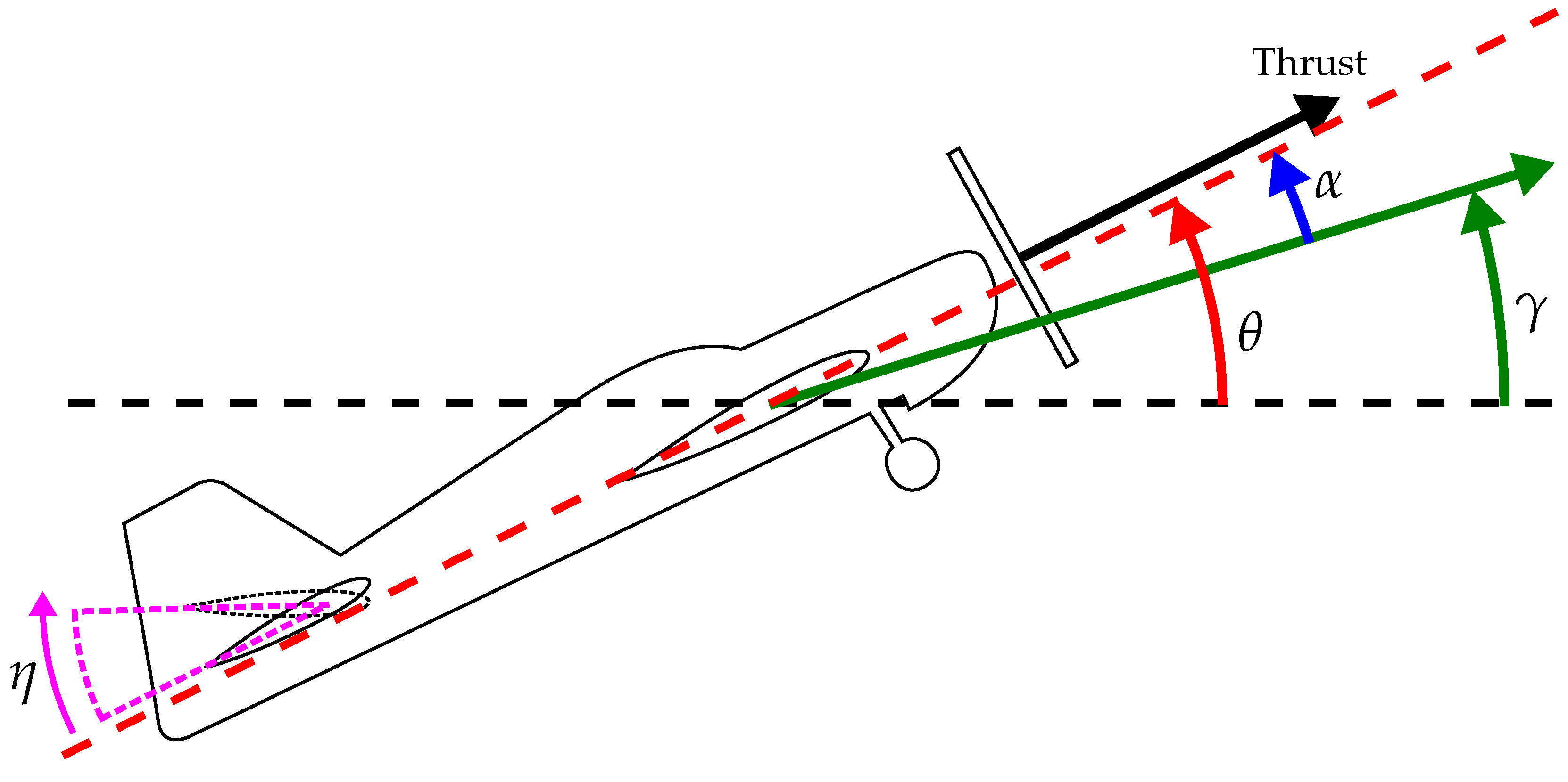
Figure 1 is a graphical representation of the various angles used in aircraft dynamics. The vehicle’s centre-of-mass is travelling along the green arrow, describing the flight path. The angle γ is the angle between this direction of travel, and the horizon is the flight path angle. The angle between the horizon and the aircraft’s reference axis is the pitch angle, denoted by θ , and the difference between the pitch and flight path angles provides the angle of attack, denoted by α . The angle of attack describes the angle between the oncoming airflow and the aircraft reference axis and is key for the modelling of the aerodynamic forces and moments. The elevator angle, η , is also shown.
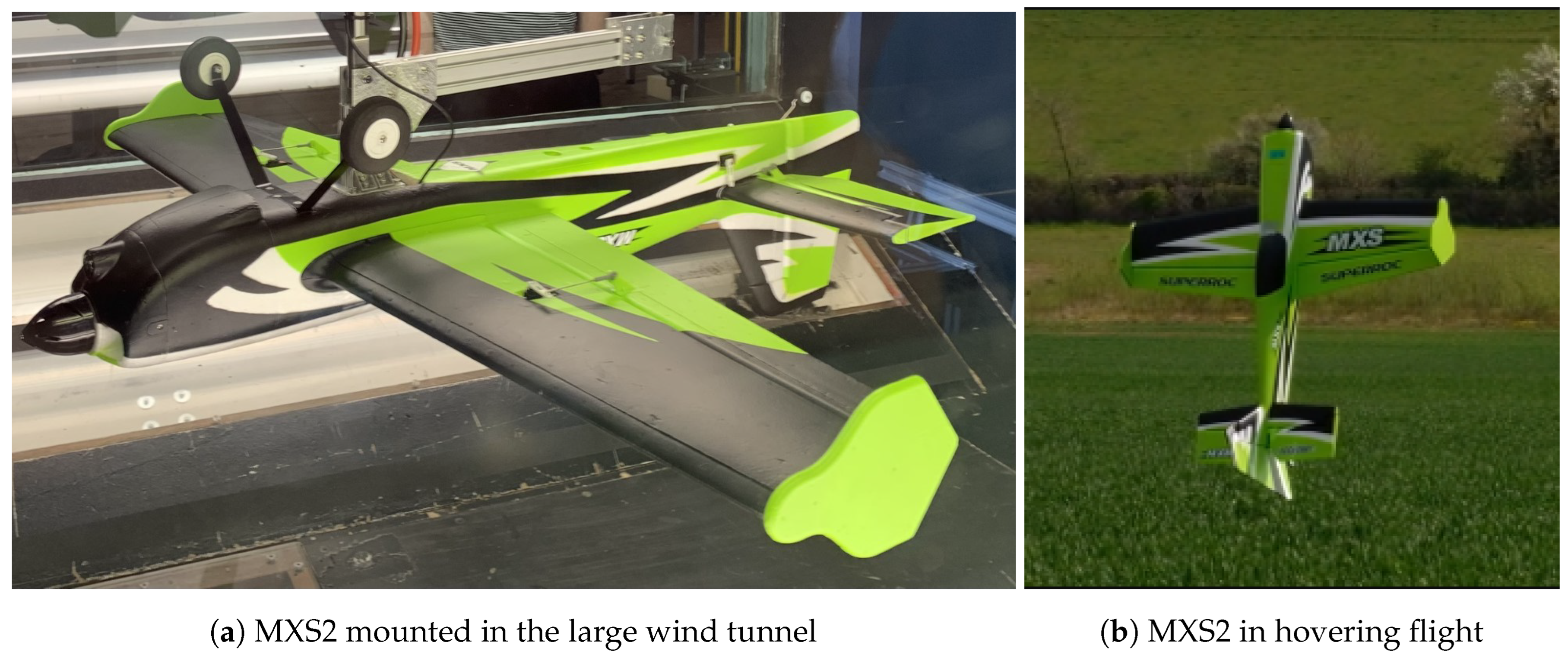
The model used in this work is based on wind-tunnel data for the FMS Models MXS2 airframe (https://www.fmshobby.com/products/fms-1100mm-mxs-v2-pnp-with-reflex, accessed on 24 November 2022), pictured in Figure 2. The airframe was mounted in the University of Bristol’s 7′ × 5′ wind tunnel, with a load cell mounted internally (see Figure 2a). Automated control inputs were generated by a set of Python scripts, which also recorded load cell data. The pitch and yaw traverse, and the tunnel airspeed, were controlled by the wind tunnel’s existing control system, which was manually provided with setpoints.
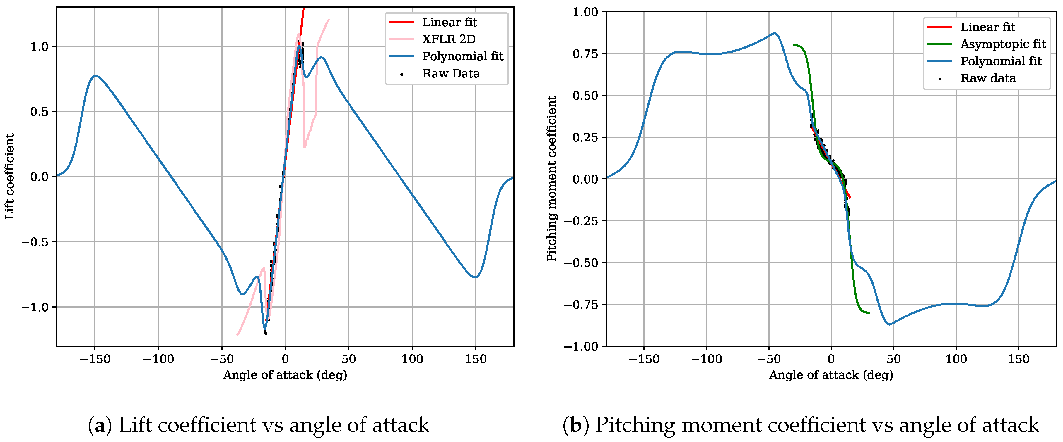
With the airframe mounted, the overall range available for the traverse was 18 to 20 in angle of attack, and ± 30 in sideslip. Data was gathered at indicated wind tunnel speeds of 10 m s−1 to 22.5 m s−1 in 2.5 m s−1 increments. The elevator, rudder and aileron were each deflected individually across a range of throttle settings at each tunnel speed and vehicle attitude, yielding a large dataset covering almost all of the conventional flight envelope and initial stages of the post-stall regime.
This data was then used to generate a set of parameterised curves to define the coefficients for the longitudinal model. These curves were extended with data from additional references to cover the full range of angle of attack from 180 through to 180 . The resulting curves for the lift and pitching moment coefficients are plotted in Figure 3.
The longitudinal model has two control inputs available: elevator angle, η and throttle setting τ . Figure 1 shows the elevator angle, here defined as the angle to which the elevator is deflected upwards relative to its neutral position. Note that this definition of elevator angle is opposite in sense to convention, generating a positive pitching moment with a positive deflection. The wind tunnel data was used to generate a coefficient for the elevator that varied with throttle setting, airspeed and elevator angle. The throttle setting is mapped to the generated thrust, based on a two-dimensional polynomial incorporating the airspeed.
Along with the forces and torques exerted on the body, the mass and inertial properties of the body are required. A second airframe was fitted with necessary hardware for autonomous flight and used to make measurements of these properties. The resulting measurements are presented in Table 1. In the work presented here, only a longitudinal model is used, so only the pitch inertia I y y and overall mass are needed.
These coefficient curves, thrust modelling and inertial data were used to implement the model using pyaerso [18]. This is an accessible Python interface to a simple flight dynamics modelling library implemented in Rust [19]. It allows forces and moments to be calculated in Python, based on the current vehicle aerodynamic state, and to be transferred to dedicated, pre-compiled machine-code for the state propagation process. Wind and atmospheric density models can also be defined in Python, or a set of pre-built models can be selected from. This allows easy experimentation without the need to recompile software or manipulate aircraft model configuration files. It also means users are free to use arbitrary functions to define their models, rather than being limited to a set supported by the underlying dynamics code. The Python interface (https://github.com/rob-clarke/pyaerso, accessed on 14 July 2023) and the underlying Rust library (https://github.com/rob-clarke/aerso, accessed on 14 July 2023) are both available on GitHub under MIT licenses.

3. Reinforcement Learning-Based Results and Discussion

3.1. Descent Manoeuvre

The initial manoeuvre explored and presented here was constrained descent. For this manoeuvre the objective is to achieve the maximum descent within a fixed forward distance, with the vehicle starting in trimmed level flight. The naïve implementation simply provides a reward proportional to the final z-coordinate value when the vehicle crosses the x-coordinate limit. In typical aerospace convention, positive z is downwards so R = w z z gives an increasing reward for increasing descent, assuming w z > 0 .
Such an implementation induces descent behaviour, with one potential solution being a vertical dive. This can achieve an unlimited descent within a fixed forward distance. However, it has a number of problems. Firstly, increasing airspeed in the dive likely exceeds the validity of the model, and in the real world could potentially exceed airframe limits. Secondly, as the episode ends when the forward distance limit is reached, the agent seeks to maximise downwards velocity in the moments before episode end in order to maximise the reward. This likely leads to an extreme nose-down attitude, which is not conducive to continued controlled flight.
To address these problems, consider the manoeuvre in the context of an approach to landing. The exit velocity should be limited, lest the vehicle overrun the runway, and the exit attitude should be close to level, assuming a conventional landing. Therefore, the exit attitude condition can be encouraged with the reward function
R end = ( 1 w θ | θ θ target | ) w z z ,
where the overall reward is weighted by the pitch error. In this case, θ target is 0, with a weighting term w θ left for tuning the reward function.
The airspeed condition can be incorporated in a similar fashion by weighting the overall reward by the ratio of the vehicle’s initial kinetic energy to that at the end of the episode:
R end = w z z | v b , 0 | 2 | v b , end | 2 .
In this formulation, an increase in the vehicle’s kinetic energy over the initial value causes a decrease in the reward, while a reduction in energy increases the reward. This has the effect of encouraging a bleed-off of energy during the manoeuvre, but this is ideal as part of a landing approach manoeuvre.
With both of these modifications in place, there is still an edge case that the agent can exploit. Assuming there is sufficient forwards distance, the vehicle can be put into a potentially unlimited vertical dive and pull up into a climb to bleed off the excess energy prior to hitting the forward limit. This is not a particularly useful solution in an approach to landing scenario, unless the landing site is located on a cliff edge. To combat this, the reward function is further augmented to penalise the amount of climb the vehicle carries out during the manoeuvre:
R end = w z z 1 + w climb ( z max z ) .
This reduces the award for any end position above the lowest point in the manoeuvre. The w climb parameter is used for tuning the reward.
There are a few further edge cases that the agent could exploit that are imposed with hard limits, rather than modifying the shape of the end-of-episode reward. If any of the conditions are breached, the episode is ended immediately and a negative reward given to the agent. First, there is a lower limit on the x-coordinate to prevent the agent using more forwards space than intended by flying the aircraft back past the initial position. Second, there is a set of conditions to prevent the agent looping the vehicle. This could come about in a similar fashion to the scenario requiring climb mitigation, where a vertical dive can be recovered into a high angle-of-attack (and so a high drag) loop, allowing bleed-off of energy without triggering the reward penalty for climbing introduced above. An outline of this hypothetical manoeuvre sequence is shown in Figure 4. Finally, an effort was made to keep the simulation within the range of validity for the model by putting limits on the vehicle’s body–axis velocity. For future experiments with wind incorporated, this will need to be modified to reflect the vehicle airspeed. These limitations are represented mathematically in Equation (7).
R end = ( 1 w θ | θ | ) z k ( 1 + w climb ( z max z ) ) if x > x lim 1000 if x < 0 1000 if θ > 89 or θ < 270 1000 if u > u lim or u < 0 k = | v b , end | 2 | v b , 0 | 2
Figure 5a,b show a position plot and the vehicle state traces for an evaluation of an agent trained on the reward function in Equation (7). Table 2 lists the parameters used during training. Note the pitch weight of 0, meaning that error in pitch did not discount the reward. The pitch-up behaviour at the end of the episode was likely due to the high angle of attack causing significant energy loss, so the agent pitched up to reduce the reward discount due to energy gain. The initial use of high throttle was likely to increase elevator response in order to rapidly pitch the aircraft nose down.

3.2. Adding Waypoints to the Descent Manoeuvre

For Figure 6 waypoints were added to the scenario and the x-distance available for the manoeuvre extended out to 45 m. The purpose of this scenario was to demonstrate the use of additional requirements on the manoeuvre during the descent. The aircraft can be seen to pitch up to meet the first waypoint before rapidly pitching nose down to meet the second. The success of this type of manoeuvre is highly dependent on the weighting given to the waypoints, relative to the requirements for the descent and the exit from the episode. The waypoints themselves influenced the RL, based on proximity to the waypoint, until each x-coordinate was passed, using the reward function
R end = R descent + t = 0 T r wp , r wp = w wp i = 1 n wp 0 x > x wp i 1 | ( x , z ) ( x , z ) wp i | + 0.01 otherwise .
Note that, unlike the overall manoeuvre reward, the waypoint reward was delivered continuously throughout the episode. This meant careful balancing of the waypoint weight, and w wp , was required to ensure that the reward signal from the waypoints did not overpower the final episode reward. For the result presented above, w w p was set to 0.15. This resulted in the waypoint-derived reward being 52% of the total reward for the episode. The other parameters used in training are listed in Table 3.

3.3. Hover Manoeuvre

The next manoeuvre explored and presented here is a hover entry. The main objective was for the agent to control the vehicle from level trimmed flight through to a hover. There was an ‘easy’ solution in the vehicle pitching to the vertical and maintaining that attitude until the speed reduced to 0. In order to provide a more interesting environment and challenge, a secondary objective was also encoded into the reward function.
Initially, this secondary objective was to minimise the height gain during the manoeuvre. To motivate this, again consider the manoeuvre as part of an approach to a landing sequence, this time for a tail-sitter landing. The hover condition is much less efficient than conventional flight, so to minimise energy expenditure during the final descent phase, the transition to hovering flight should take place as low as possible.
The initial approach was to check at each timestep if the vehicle had achieved a state within some acceptable bounds of a hover, with the assumption that a conventional control system would then be able to stabilise the hover. The bounds used for the hover state are listed in Table 4. If the vehicle was deemed to be in the hover, the episode was ended and the episode reward was proportional to the final height of the vehicle: namely, R = z end + c . The constant offset was tuned to ensure that heights above the starting position (that is a negative z-coordinate) did not result in a negative reward.
This initial approach proved difficult to train. Most runs resulted in the vehicle simply falling until the episode was terminated by the time or position limits. The reward signal was only given in the constrained part of the state space near the hover condition, which made it very sparse for the learning algorithm, with the gradient in the reward space difficult to determine. In order to improve this, a time limit was added to the episodes, after which the reward would be based on the vehicle’s progress towards the hover state, as shown in the reward function
R end = 100 1 1 + | q | · 1 1 + | 90 θ | · 1 1 + | u | · 1 1 + | w | .
For a perfect hover, this function returned a value of 100, with any deviation from hover discounting this. The constant offset above was also tuned to ensure a successful hover resulted in a reward greater than 100.
Figure 7a,b show the evaluated outputs for an agent trained with the hover reward function. The parameters used for training the agent are listed in Table 5. The horizontal velocity at the end of the episode was still a little high for the hover condition, so the episode timed out. Of note was the initial throttle input, which was likely to increase elevator effectiveness. This was followed by a period of no throttle to minimise height gain. The throttle then increased at the end of the episode to maintain the hover. The overall height gain throughout the manoeuvre was ≈ 10 m. Note also the rapid transition into the high alpha regime as the throttle came back on at approximately 1.8 s.
During training for this manoeuvre, another solution was generated in addition to the expected aggressive pitch-up, this being a nose-down manoeuvre. In the nose-down variation, the vehicle pitches down, passing through extreme negative angles of attack before ending the episode pointing upwards, usually significantly below the starting point and, potentially, very close to the hover condition. This drop below the starting point yields a significant improvement in reward over the more conventional approach. A successful execution of the nose-down variation has not been seen in a final deterministic evaluation. It would be interesting to see if this nose-down variation is physically realisable, and whether the aircraft model accurately captures the physics at these very high negative angles of attack. It would also be intriguing to witness how the learning algorithms find unexpected solutions to maximise the reward function.
The runs that exploit this manoeuvre typically initially exhibit a high throttle with minimal pitch input, serving to accelerate the vehicle. This increased airspeed increases the pitch authority of the elevator, which the agent then uses to rapidly pitch down. In some cases, the angular momentum from the pitch input is just sufficient to transition the vehicle through 90 angle of attack and into a nose-up attitude. However, typically, the final deterministic evaluation does not show sufficient momentum to complete the transition through to the nose-up state.

3.4. Turn-Around and Climb Manoeuvres

Two additional manoeuvres are also presented here, in less detail. The first is a turn-around manoeuvre, to reverse the direction of travel. The second is a climb within a fixed forward distance.
In previously presented cases, the agent learnt using the full six-degree-of-freedom state of the vehicle. However, the model is only longitudinal, so many members of the observation vector are unchanging. Truncating the state vector to only include the relevant longitudinal states should allow the agent to begin learning relevant information sooner, rather than learning to ignore unchanging state–vector elements. This approach was followed for the direction change and climb manoeuvres.

3.4.1. Turn-Around Manoeuvre

For the turn-around manoeuvre, the objective is to reverse the direction of travel of the vehicle. As the model is restricted to the longitudinal plane, this means the vehicle ends the manoeuvre inverted.
To minimise the constraints on the agent, the reward function was initially specified very loosely, only requiring that the vehicle x-coordinate became negative. This was later augmented to include a penalty for ending the manoeuvre at a different height than it was started at, and penalising longer episode times. Combined, these had the effect of influencing the agent to complete the manoeuvre as quickly as possible, with minimal change in height.
The reward function for the turn-around manoeuvre is
R end = 1 + 1 T 100 w z ( 1 + | z | ) .
This reward was applied at the end of the episode, determined by the point where the x-coordinate went below 0. For all other time steps, the returned reward was zero. The value T represents the number of time steps in the episode.
Figure 8 shows an example evaluation of the turn-around manoeuvre. The parameters used in training the agent are listed in Table 6 The height change penalty appears to be disproportional to the time-based penalty as there is a significant height change throughout the manoeuvre.

3.4.2. Climb Manoeuvre

The second additional manoeuvre demonstrates a climb within a fixed forward distance. During this manoeuvre, the response is penalised if the u velocity drops below 7 m s−1 and the pitch angle is rewarded for being zero at the end of an episode. Figure 9 shows an example evaluation and the aircraft can be seen to transition into a climb, whilst maintaining airspeed. The agent was trained using the parameters listed in Table 7. Although the pitch angle can be seen to be reducing towards the end, it did not level out. This was likely to be due to insufficient pitch weight in the reward function, given in Equation (8). It can also be noted that this agent took approximately 20 min to train on a standard laptop. It would be possible to extend the flight time of each episode and increase the weighting on the pitch angle response which would allow for transition into, and out of, the climb.
R end = z + 10 ( 1 w θ | θ | )

3.5. Learning Multiple Manoeuvres with a Single Network

This section takes a single network and trains it for two different manoeuvres. The objective is to train the agent with an additional input to encode the manoeuvre that is being demanded. Hence, the manoeuvre is encoded as an ’one-hot’ vector in addition to the standard state data. This vector encodes the selected manoeuvre as a single 1 value within a vector of zeroes. As with the turn-around and climb manoeuvres, a truncated state vector is used, containing only the longitudinal state elements. For the purposes of this demonstration, the descent and hover entry manoeuvres, that have been shown in the sections above, were selected.
The agent is trained on both manoeuvres simultaneously, alternating between them, with the manoeuvre encoding input and the reward function changing for each episode. This allows the single network agent to be exposed equally to training data for both manoeuvres.
The agent was trained on both descent and entry into the hover using the settings as detailed in Table 8. The simulation results from this can be seen in Figure 10. Starting from identical flight conditions, the aircraft can be seen transitioning into the hover and into a descent depending on the the ‘one-hot’ state input used.
In this case, though, ‘bleed’ can be seen between the manoeuvres where, for example, the descent manoeuvre ended with the aircraft at a very high angle of attack, whereas a low pitch angle and alpha response was desirable. During experimentation, it was found that increased network depth improved the discrimination between manoeuvres. Therefore, a depth of 3, one additional layer, was used for the multi-manoeuvre cases.
In the following example, the pitch weight was used to penalise the high pitch at the end of the descent manoeuvre, to aid the agent in discriminating between the required behaviours. Following this, the two manoeuvres from a single agent were linked together sequentially.

3.6. Linking Manoeuvres

Prior to demonstrating the sequential response of the two separate manoeuvres from a single agent, it was retrained with an increased pitch angle weight, and with noise applied to the starting conditions. As with the previous example, the selected manoeuvre was encoded with a ‘one-hot’ vector appended to the truncated longitudinal state vector. The increase in the pitch angle weight reduced the ‘bleed’ between the manoeuvres and allowed for a smoother transition between the two manoeuvres when linked sequentially. The added noise allowed for imperfect state conditions at the start of the episode, which would arise when linking together the manoeuvres sequentially. Although these combined changes could result in a poorer overall performance, signified by a lower overall reward function, the agent was more robust to noise in the starting state and demonstrated clearer separation between the two manoeuvres.
The noise added to the starting conditions was distributed uniformly within a range defined by the run metadata. The values given for airspeed and flight path angle noise in Table 9 were the half-range of this distribution. For example, the airspeed value used for each episode was distributed uniformly within a range ± 1.0 m s−1 about the trimmed airspeed.
Figure 11 shows the new response for the agent trained on two manoeuvres. The improvement can clearly be seen in the pitch angle response where the aircraft was much closer to having a pitch angle of zero for the descent at the end of the episode, and much closer to the vertical at the end of the episode when that manoeuvre was demanded. It is this instance of the trained agent that was used in the final demonstration where both manoeuvres were demonstrated sequentially in the same simulation.
The manoeuvres were chained together by transforming the vehicle’s position for the second manoeuvre, such that the manoeuvre appeared to start at position ( x , z ) = ( 0 , 0 ) , replicating the conditions experienced during training. This transformation is represented in Equation (9). The remainder of the state vector remained untransformed. The simulation of this run can be seen in Figure 12, where the aircraft initially descended, and, at the conclusion of this first manoeuvre, the agent was signalled to transition into the vertical. It should be noted that the entry speed into the hover was faster than the agent experienced during the training episodes, which was why the aircraft was close to the vertical, but still at non-zero airspeed at the conclusion of both manoeuvres.
( x , z ) = ( x x T 1 , z z T 1 )
The scenario shown here could represent transition through an opening into a confined space. It should be noted that the obstacles shown in the figure were not used within the simulation, but were used to demonstrate how these types of agents could be used in practice. With robust responses, multiple manoeuvres and agents could be chained together to create complex, nonlinear paths, capable of fast responses with lightweight controller implementation.

4. Conclusions and Further Work

A new nonlinear aircraft model was used within a reinforcement learning framework to train agents to perform different longitudinal manoeuvres, including those at a high angle of attack where response is highly nonlinear. The approach taken is shown to be able to encode for manoeuvres including transition into the hover and the descent. Furthermore, a single agent was trained for two manoeuvres, which were subsequently demonstrated in a single simulation where both were performed sequentially.
There are many avenues available for further work, including additional randomisation, both on the input state and in the simulation environment in which the agents are trained. This should include the effects of gusts and steady state wind. The results shown here are for the longitudinal response. It would be interesting to extend the training to include the lateral-directional response, to allow for nonlinear flight regimes such as the spin.
Whilst the model is based on both wind tunnel data and additional resources, it would be useful to further explore the fidelity at high alpha. This would also benefit from taking the model and the trained agents into free-flight. One reason for the selection of the baseline aircraft is that it is available for free flight tests in the same configuration that it was tested in the wind tunnel. Comparison of simulated and free-flight data through manoeuvres and model identification from free-flight data will help to highlight continuing model inaccuracies and the remaining reality gap.
Training the model for multiple manoeuvres comes at the expense of increased training time. The trade-off between the use of linked multiple agents for simplicity, against the use of a larger network single agent needs to be evaluated through manoeuvre performance, training time, overall weight size and robustness. Increased randomisation of the initial conditions would allow a single agent to cope with variation in the end points. Increased training with stricter conditions on the endpoints would also help to facilitate robust transition between manoeuvres. The networks would also benefit from further hyper-parameter optimisation. The use of eXplainable AI (XAI) methods may help in this optimisation effort, and in assessing the efficacy of the current approach. The use of such methods in a control context, with coupled input states, is an area of active research [5,20].
Finally, reinforcement learning-based agents were shown to be capable of exploiting the high-alpha part of the flight envelope through rapid manoeuvres. This was achieved through the use of complex reward structures, and our future work will consider the inclusion of these agents in a multi-modal form of control where there are transitions between more traditional model predictive control and the rapid manoeuvres that this type of agent can generate. Flight into, and out of, confined spaces with fixed-wing vehicles will benefit from rapid, nonlinear, agile control structures.

Author Contributions

Investigation and methodology, R.C. and L.F.; software and visualization, R.C.; supervision T.R. and S.E.; writing R.C., T.R. and S.E. All authors have read and agreed to the published version of the manuscript.

Funding

This work was supported by the Engineering and Physical Sciences Research Council grant number EP/N509619/1.

Data Availability Statement

The code used in generating these results is available on GitHub at: https://github.com/rob-clarke/pymxs (accessed on 14 July 2023). The repository also includes the wind tunnel data and the longitudinal model implementation under the wind_tunnel_data and models directories respectively. Run data and trained models are available in the same repository in the archive branch.

Conflicts of Interest

The authors declare no conflict of interest.

References

  1. Fletcher, L.; Clarke, R.; Richardson, T.; Hansen, M. Improvements in learning to control perched landings. Aeronaut. J. 2022, 126, 1101–1123. [Google Scholar] [CrossRef]
  2. Cano Lopes, G.; Ferreira, M.; da Silva Simões, A.; Luna Colombini, E. Intelligent Control of a Quadrotor with Proximal Policy Optimization Reinforcement Learning. In Proceedings of the 2018 Latin American Robotic Symposium, 2018 Brazilian Symposium on Robotics (SBR) and 2018 Workshop on Robotics in Education (WRE), João Pessoa, Brazil, 6–10 November 2018; pp. 503–508. [Google Scholar] [CrossRef]
  3. Carvalho Melo, L.; Omena Albuquerque Máximo, M.R. Learning Humanoid Robot Running Skills through Proximal Policy Optimization. In Proceedings of the 2019 Latin American Robotics Symposium (LARS), 2019 Brazilian Symposium on Robotics (SBR) and 2019 Workshop on Robotics in Education (WRE), Rio Grande, Brazil, 23–25 October 2019; pp. 37–42. [Google Scholar] [CrossRef]
  4. Aractingi, M.; Léziart, P.A.; Flayols, T.; Perez, J.; Silander, T.; Souères, P. Controlling the Solo12 quadruped robot with deep reinforcement learning. Sci. Rep. 2023, 13, 11945. [Google Scholar] [CrossRef] [PubMed]
  5. Løver, J.; Gjærum, V.B.; Lekkas, A.M. Explainable AI methods on a deep reinforcement learning agent for automatic docking. (This work was supported by the Research Council of Norway through the EXAIGON project, project number 304843). IFAC-PapersOnLine 2021, 54, 146–152. [Google Scholar] [CrossRef]
  6. Libardi, G.; De Fabritiis, G.; Dittert, S. Guided Exploration with Proximal Policy Optimization using a Single Demonstration. In Proceedings of the 38th International Conference on Machine Learning, Vienna, Austria (Virtual), 18–24 July 2021; Meila, M., Zhang, T., Eds.; International Machine Learning Society: Princeton, NJ, USA, 2021; Volume 139, pp. 6611–6620. [Google Scholar]
  7. Bøhn, E.; Coates, E.M.; Moe, S.; Johansen, T.A. Deep Reinforcement Learning Attitude Control of Fixed-Wing UAVs Using Proximal Policy optimization. In Proceedings of the 2019 International Conference on Unmanned Aircraft Systems (ICUAS), Atlanta, GA, USA, 11–14 June 2019; pp. 523–533. [Google Scholar] [CrossRef] [Green Version]
  8. Bohn, E.; Coates, E.M.; Reinhardt, D.; Johansen, T.A. Data-Efficient Deep Reinforcement Learning for Attitude Control of Fixed-Wing UAVs: Field Experiments. IEEE Trans. Neural Netw. Learn. Syst. 2023; early access. [Google Scholar] [CrossRef] [PubMed]
  9. Wei, W.; Fang, Z.; Zhu, Y. Model-free Maneuvering Control of Fixed-Wing UAVs Based on Deep Reinforcement Learning. In Proceedings of the AIAA SCITECH 2023 Forum, National Harbor, MD, USA, 23–27 January 2023. [Google Scholar] [CrossRef]
  10. Clarke, S.; Hwang, I. Deep Reinforcement Learning Control for Aerobatic Maneuvering of Agile Fixed-Wing Aircraft. In Proceedings of the AIAA Scitech 2020 Forum, Orlando, FL, USA, 6–10 January 2020. [Google Scholar] [CrossRef]
  11. Lee, J.H.; Kampen, E.J.V. Online Reinforcement Learning for Fixed-Wing Aircraft Longitudinal Control. In Proceedings of the AIAA Scitech 2021 Forum, Virtual, 11–15 and 19–21 January 2021. [Google Scholar] [CrossRef]
  12. Wu, J.; Wang, H.; Liu, Y.; Zhang, M.; Wu, T. Learning-based fixed-wing UAV reactive maneuver control for obstacle avoidance. Aerosp. Sci. Technol. 2022, 126, 107623. [Google Scholar] [CrossRef]
  13. Zhang, S.; Du, X.; Xiao, J.; Huang, J.; He, K. Reinforcement Learning Control for 6 DOF Flight of Fixed-Wing Aircraft. In Proceedings of the 2021 33rd Chinese Control and Decision Conference (CCDC), Kunming, China, 22–24 May 2021; pp. 5454–5460. [Google Scholar] [CrossRef]
  14. Zhen, Y.; Hao, M.; Sun, W. Deep Reinforcement Learning Attitude Control of Fixed-Wing UAVs. In Proceedings of the 2020 3rd International Conference on Unmanned Systems (ICUS), Harbin, China, 27–28 November 2020; pp. 239–244. [Google Scholar] [CrossRef]
  15. Raffin, A.; Hill, A.; Gleave, A.; Kanervisto, A.; Ernestus, M.; Dormann, N. Stable-Baselines3: Reliable Reinforcement Learning Implementations. J. Mach. Learn. Res. 2021, 22, 1–8. [Google Scholar]
  16. Schulman, J.; Wolski, F.; Dhariwal, P.; Radford, A.; Klimov, O. Proximal Policy Optimization Algorithms. arXiv 2017, arXiv:1707.06347. [Google Scholar]
  17. Schulman, J.; Levine, S.; Abbeel, P.; Jordan, M.; Moritz, P. Trust Region Policy Optimization. In Proceedings of the 32nd International Conference on Machine Learning, Lille, France, 7–9 July 2015; Bach, F., Blei, D., Eds.; International Machine Learning Society: Princeton, NJ, USA, 2015; Volume 37, pp. 1889–1897. [Google Scholar]
  18. Clarke, R.J.; Fletcher, L.J.; Richardson, T.S. pyaerso: A Rust-backed Python Module for Accessible Flight Dynamics Modelling for Machine Learning. In Proceedings of the AIAA SCITECH 2023 Forum, National Harbor, MD, USA, 23–27 January 2023. [Google Scholar] [CrossRef]
  19. Matsakis, N.D.; Klock, F.S., II. The rust language. ACM Sigada Ada Lett. 2014, 34, 103–104. [Google Scholar] [CrossRef]
  20. Raz, A.K.; Nolan, S.M.; Levin, W.; Mall, K.; Mia, A.; Mockus, L.; Ezra, K.; Williams, K. Test and Evaluation of Reinforcement Learning via Robustness Testing and Explainable AI for High-Speed Aerospace Vehicles. In Proceedings of the 2022 IEEE Aerospace Conference (AERO), Big Sky, MT, USA, 5–12 March 2022; pp. 1–14. [Google Scholar] [CrossRef]
Figure 1. Diagram showing definitions of pitch angle, θ , angle of attack, α , flight path angle, γ , and elevator angle, η .
Algorithms 16 00384 g001
Figure 2. Images of the MXS2 airframe in the University of Bristol Wind Tunnel and in free flight at the University of Bristol Fenswood free flight facility.
Algorithms 16 00384 g002
Figure 3. Plots of the lift and pitching moment coefficient curves used in the MXS model across the full range of α .
Algorithms 16 00384 g003
Figure 4. Diagram showing a hypothetical looping exit from a vertical dive.
Algorithms 16 00384 g004
Figure 5. Run A: Simulation results showing Reinforcement Learning-based Descent Response.
Algorithms 16 00384 g005
Figure 6. Run B: Simulation results showing the Descent Response With Waypoints.
Algorithms 16 00384 g006
Figure 7. Run C: Simulation results showing the transition into the Hover.
Algorithms 16 00384 g007
Figure 8. Run D: Simulation results showing the Turn-around Manoeuvre.
Algorithms 16 00384 g008
Figure 9. Run E: Simulation results showing the Climb manoeuvre response.
Algorithms 16 00384 g009
Figure 10. Run F: Simulation results showing the Multiple Manoeuvres from a Single Agent.
Algorithms 16 00384 g010
Figure 11. Run G: Simulation demonstrating Multi-manoeuvre Agent with noise.
Algorithms 16 00384 g011
Figure 12. Run G: multi-manoeuvre with noise sequentially evaluated output. Shown with representative obstacles.
Algorithms 16 00384 g012
Table 1. Mass and inertial properties of the MXS2 airframe.
PropertyMeasuredUnit
Mass, m1.221 kg
I x x 0.019 kg m 2
I y y 0.091 kg m 2
I z z 0.121 kg m 2
Table 2. Run A: Descent metadata used.
ParameterValue
Timesteps500,000
x lim 30 m
u lim 25 m s−1
w θ 0
w climb 1
Table 3. Run B: Descent with Waypoints metadata used.
ParameterValue
Timesteps500,000
x lim 45 m
u lim 25 m s−1
w θ 0
w climb 1
w wp 0.15
Waypoint positions ( 10 , 2 ) and ( 30 , 5 )
Table 4. Limits on state variables for hover condition check.
ParameterLower LimitUpper Limit
Pitch angle, θ 85 95
Pitch rate, q 0.01 rad s−1 0.01 rad s−1
x-axis velocity, u 0.1 m s−1 0.1 m s−1
z-axis velocity, w 0.1 m s−1 0.1 m s−1
Table 5. Run C: Hover metadata used.
ParameterValue
Timesteps1,500,000
x lim 30 m
u lim 25 m s−1
Table 6. Run D: Turn-around metadata used.
ParameterValue
Timesteps500,000
x lim 30 m
u lim 25 m s−1
w climb 1
Use reduced observationTrue
Table 7. Run E: Climb metadata used.
ParameterValue
Timesteps500,000
x lim 30 m
u lim 25 m s−1
w θ 0
Use reduced observationTrue
Table 8. Run F: Multi-manoeuvre metadata used.
ParameterValue
Timesteps1,000,000
x lim 30 m
u lim 25 m s−1
w θ 0
w climb 1
Use reduced observationTrue
Network depth3
Network width64
Table 9. Run G: Multi-manoeuvre with noise metadata used.
ParameterValue
Timesteps1,000,000
x lim 30 m
u lim 25 m s−1
w θ 1
w climb 1
Use reduced observationTrue
Network depth3
Network width64
Airspeed noise 1.0 m s−1
Flight path angle noise 0.2 rad
Disclaimer/Publisher’s Note: The statements, opinions and data contained in all publications are solely those of the individual author(s) and contributor(s) and not of MDPI and/or the editor(s). MDPI and/or the editor(s) disclaim responsibility for any injury to people or property resulting from any ideas, methods, instructions or products referred to in the content.

