Article

Iterative Oblique Decision Trees Deliver Explainable RL Models

1
Cologne Institute of Computer Science, Faculty of Computer Science and Engineering Science, TH Köln, 51643 Gummersbach, Germany
2
Institute for Neural Computation, Faculty of Computer Science, Ruhr-University Bochum, 44801 Bochum, Germany
*
Author to whom correspondence should be addressed.
Algorithms 2023, 16(6), 282; https://doi.org/10.3390/a16060282
Submission received: 25 April 2023 / Revised: 25 May 2023 / Accepted: 30 May 2023 / Published: 31 May 2023
(This article belongs to the Special Issue Advancements in Reinforcement Learning Algorithms)

Abstract

:
The demand for explainable and transparent models increases with the continued success of reinforcement learning. In this article, we explore the potential of generating shallow decision trees (DTs) as simple and transparent surrogate models for opaque deep reinforcement learning (DRL) agents. We investigate three algorithms for generating training data for axis-parallel and oblique DTs with the help of DRL agents (“oracles”) and evaluate these methods on classic control problems from OpenAI Gym. The results show that one of our newly developed algorithms, the iterative training, outperforms traditional sampling algorithms, resulting in well-performing DTs that often even surpass the oracle from which they were trained. Even higher dimensional problems can be solved with surprisingly shallow DTs. We discuss the advantages and disadvantages of different sampling methods and insights into the decision-making process made possible by the transparent nature of DTs. Our work contributes to the development of not only powerful but also explainable RL agents and highlights the potential of DTs as a simple and effective alternative to complex DRL models.

1. Introduction

One of the most significant drawbacks of powerful deep reinforcement learning (DRL) algorithms is their opacity. The well-performing decision-making process is buried in the depth of artificial neural networks, which might constitute a major barrier to the application of reinforcement learning (RL) in various areas.
In a recent publication [1], we proposed an algorithm for obtaining simple decision trees (DTs) from trained DRL agents (“oracles”). The basic idea is to observe how a trained DRL agent acts in an environment while logging the data pairs (state, action) as samples. These samples are then used to train a DT to predict actions with high accuracy. This approach has notable advantages:
  • It is conceptually simple, as it translates the problem of explainable RL into a supervised learning setting.
  • DTs are fully transparent and (at least for limited depth) offer a set of easily understandable rules.
  • The approach is oracle-agnostic: it does not rely on the agent being trained by a specific RL algorithm, as only a training set of state–action pairs is required.
Although the algorithm in [1] was successful on some problems, it failed on others because no well-performing shallow DT could be found. In this work, we investigate the reasons for those failures and propose three algorithms to generate training samples for the DTs: The first one is entirely based on evaluation episodes of the DRL agent (described in [1] and evaluated further in this article), the second one applies random sampling on a subregion of the observation space, and the third approach is an iterative algorithm involving the DRL agent’s predictions for regions explored by the DT. We test all approaches on seven environments of varying dimensionality, including all classic control problems from OpenAI Gym. Our results show that DTs of shallow depth can solve all environments, that DTs can even surpass DRL agents, and that the third algorithm (the iterative approach) outperforms the other two methods in finding simple and well-performing trees. As a particularly surprising result, we show that an 8-dimensional control problem (LunarLander) can be successfully solved with a DT of only depth 2.
To achieve these results, we had to address the challenges of sampling data from an oracle in a way that would be useful for tree learning. The first challenge is that data from successful oracle episodes may have regions of severe oversampling in the state space. For example, an agent being successful in pole balancing will have most samples concentrated in a small region around the unstable equilibrium. These samples are not only redundant for tree learning but will overshadow the other samples that are important to perform a successful episode. The second challenge is that data from successful episodes may omit regions in state space that are physically reachable but never visited by those episodes. These are regions that a successful agent has learned to avoid because they are unfavorable. As a consequence, it does not transmit the knowledge of the right action to the samples, and thus the decision tree will likely not take the right action in those regions. We will describe in Section 3 several methods to address these challenges.
Explainable artificial intelligence (XAI) is becoming increasingly significant today. This is because one wants to bring artificial intelligence applications into practice in a way that ensures reliable and trustworthy models. The reason that we want to build successful DTs is that they represent simple models that offer various options for explainability that opaque DRL models do not have. We will discuss in Section 4 the advantages and disadvantages of the three algorithms’ computational complexity and how the transparent, simple nature of DTs provides interesting options for explainability that are not directly applicable to non-transparent DRL models.
The remainder of the article is structured as follows: In Section 2, we present related work. Section 3 contains a detailed description of our methods and the experimental setup. In Section 4, we present our results and discuss the explainability of DTs. We place our results in a broader context and discuss future research in Section 5 before drawing a short conclusion in Section 6.

2. Related Work

In recent years, interest in explainable and interpretable algorithms for Deep Learning algorithms has grown steadily. This is shown by review articles for XAI and explainable machine learning in general [2,3,4] and, more recently, by review articles for explainable reinforcement learning (XRL) in particular [5,6,7]. Lundberg et al. [8] give an overview of efficient algorithms for generating explanations, especially for trees.
A variety of rule deduction methods have been developed over the years. Liu et al. [9] apply a mimic learning approach to RL using comparably complex Linear Model U-trees to approximate a Q-function. Our approach differs insofar as the DTs we obtain are arguably simpler and represent a transparent policy, translating state into action. Mania et al. [10] propose Augmented Random Search, another algorithm for finding linear models that solve RL problems. Coppens et al. [11] distill PPO agents’ policy networks into Soft Decision Trees [12] to obtain insights. Another interesting approach to explainable RL, which does not use DTs, is the approach by Verma et al. [13] called Programmatically Interpretable RL (PIRL) through Neurally Directed Program Synthesis (NDPS). In this method, the DRL guides the search of a policy consisting of specific operators and input variables to obtain interpretable rules mimicking PID controllers. As Verma et al. [13] also test their algorithms on OpenAI Gym’s classic control problems, a direct comparison is possible and was made in [1]. However, their results were not reproducible by us (see Appendix A) and we show how our algorithms yield better results at low DT depths than the reported ones. An oracle-free approach is the programmatic RL of Qiu and Zhu [14]. Their method consists of relaxing the discrete architecture space of a programmatic policy to be continuous and subsequently optimizing policy parameters and architecture by applying gradient methods based on reward. It will be an interesting task for future work to apply our methods to environments used in their approach (OpenAI Gym MuJoCo). One of our algorithms presented in this article (ITER, Section 3.4.3) has strong similarities to the DAgger algorithm described by Ross et al. [15] regarding the aggregation of the dataset. They do, however, not use DRL algorithms for the predictions nor DTs as classifiers. They benchmark their method using image feature inputs of two video games and a handwriting recognition task. This approach was later extended by Bastani et al. [16] to leverage the Q-function of the DRL oracle. They describe an algorithm to train DTs (they use the axis-parallel CART) and test their methods, among others, on the shorter CartPole version with 200 timesteps, for which they found a CART of depth 1 with perfect return. Zilke et al. [17] propose an algorithm for distilling DTs from neural networks. With their method “DeepRED”, the authors translate each layer of a feedforward network into rules and aim to simplify those.
The work presented here extends our earlier research in [1]. We apply it to additional environments and introduce new sampling algorithms to overcome the drawbacks of [1]. To the best of our knowledge, no other algorithms are available in the current state of the art to construct simple DTs from trained DRL agents for a large variety of RL environments.
Concerning the iterative learning of trees outside of RL, well-known iterative meta-heuristics such as boosting and its particular form AdaBoost [18,19] exist, which are often applied to trees. However, boosting is iterative with respect to weak learners and outputs an ensemble of them, while our approach is iterative in the data, retrains many trees, and outputs only the best-performing one.
Rudin [20] has emphasized the importance of building inherently interpretable models instead of trying to explain black box models. While Rudin [20] applied this to standard machine learning models for application areas including criminal justice, healthcare, and computer vision, we try to take her valuable arguments over to the area of control problems and RL and show how we can substitute black box models with inherently transparent DTs without loss of performance. Although we use a DRL model to construct our DT, the final DT can be used in operation and interpreted without referencing the DRL model.

3. Methods

In this section, we explain our methods, starting with a short overview of the RL environments, and short subsections about DRL methods and DT algorithms. The main part of this section is the subsection about DT training methods, where we describe in detail our previous method (EPS) from [1] and two new sampling methods (BB and ITER). Finally, a subsection on the experimental setup describes the general algorithmic procedures and parameters that we use in all our experiments.
Our experiments were implemented in the Python programming language version 3.9.16 using a variety of different packages and methods described in the following (the code for the experiments can be found in the Github repository https://github.com/MarcOedingen/Iterative-Oblique-Decision-Trees (accessed on 25 May 2023)).

3.1. Environments

We test our different approaches of training DTs from DRL agents on all classic control problems and the LunarLander challenge offered by OpenAI Gym [21], and on the CartPole-SwingUp problem as implemented in [22]. This selection of environments offers a variety of simple but not trivial control tasks with continuous, multi-dimensional tabular observables and one-dimensional discrete or continuous actions. Table 1 gives an overview of the different environments used in this article. For the two environments without predefined solved-thresholds, we assigned a threshold corresponding to quick and stable swing-ups determined by visual inspection of episodes’ renderings.

3.2. Deep Reinforcement Learning

Our algorithms require a DRL agent to predict actions for given observations. We train DRL agents (“oracles”) using PPO [23], DQN [24], and TD3 [25] algorithms as implemented in the Python DRL framework Stable-Baselines3 (SB3) [26]. It is necessary to test all those algorithms because no single DRL algorithm solves all environments used in this paper.

3.3. Decision Trees

For the training of DTs, we rely on two algorithms representing two “families” of DTs: The widely-used Classification and Regression Trees (CARTs) as described by Breiman et al. [27] and implemented in [28] partition the observation space with axis-parallel splits. The decision rules use only one observable at a time, which makes them particularly easy to interpret. On the other hand, Oblique Predictive Clustering Trees (OPCTs), as described and implemented in [29], can generate DTs where each decision rule compares the weighted sum of the features o i to a threshold τ :
w 1 o 1 + w 2 o 2 + + w n o n τ
Such rules subdivide the feature space with oblique splits (tilted hyperplanes), allowing them to describe more complex partitions with fewer rules and, consequently, lower depth. However, the oblique split rules make the interpretation of such trees more challenging. We will address this topic in Section 4.4.

3.4. DT Training Methods

In this subsection, we describe our different algorithms to generate datasets of samples for the training of DTs.

3.4.1. Episode Samples (EPS)

The basic approach has been described in detail in [1]. In brief, it consists of three steps:
  • A DRL agent (“oracle”) is trained to solve the problem posed by the studied environment.
  • The oracle acting according to its trained policy is evaluated for a set number of episodes. At each time step, the state of the environment and action of the agent are logged until a total of n s samples are collected.
  • A decision tree (CART or OPCT) is trained from the samples collected in the previous step.

3.4.2. Bounding Box (BB)

Detailed investigations of the failures of DTs trained on episode samples for the pendulum environment show that a well-performing oracle only visits a very restricted region of the observation space and oversamples specific subregions. A good oracle is able to swing the pendulum in the upright position quickly and keeps the system in a small region around the corresponding point in the state space for the rest of the episode’s duration.
To counteract this issue, we investigated an approach based on querying the oracle at random points in the observation space. The algorithm consists of three steps:
  • The oracle is evaluated for a certain number of episodes. Let L i and U i be the lower and upper bound of the visited points in the ith dimension of the observation space and IQR i their interquartile range (difference between the 75th and the 25th percentile).
  • Based on the statistics of visited points in the observation space from the previous step, we take a certain number n s of samples from the uniform distribution within a hyperrectangle of side lengths L i 1.5 · IQR i , U i + 1.5 · IQR i . The side length is clipped, should it exceed the predefined boundaries of the environment.
  • For all investigated depths d, OPCTs are trained from the dataset consisting of the n s samples and the corresponding actions predicted by the oracle.
It should be noted that this algorithm has its peculiarities. Randomly chosen points in the observation space might correspond to inconsistent states. While this is evident for the example of Pendulum (the observations contain cos θ and sin θ (see Table 1), which was solved here by sampling θ and generating observations from that), less apparent constraints between observables may occur in other cases. We cannot guarantee that we will always generate samples that meet the constraints. We found Algorithm BB to still work if constraint-violating samples are added, but the oracle may be evaluated at points that cannot occur in actual episodes. Such evaluations may lead to performance degradation of BB. This limitation exists only for algorithm BB, not for EPS or ITER, and was, in fact, one of the main reasons for developing the ITER algorithm, which we describe in the next section.

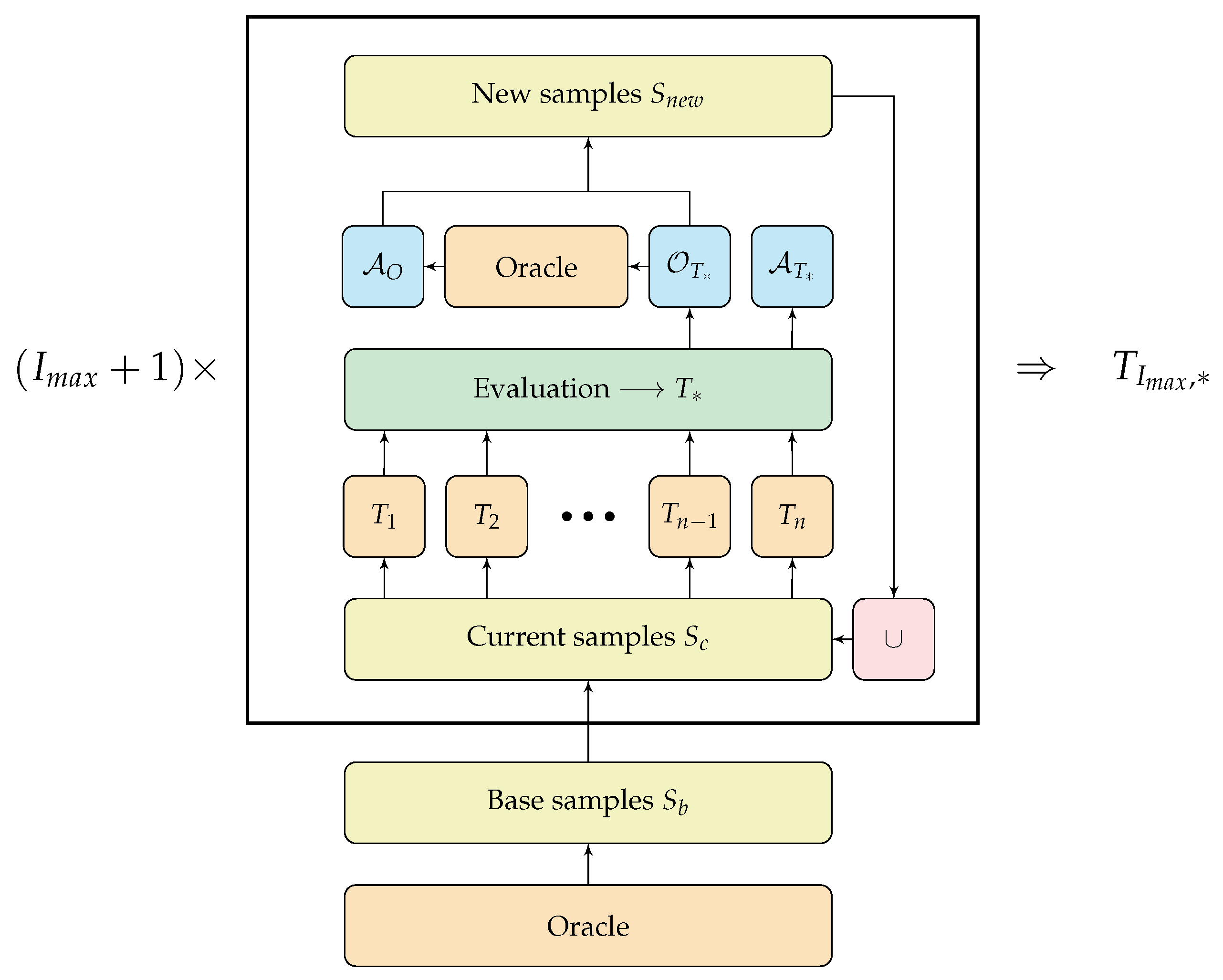
3.4.3. Iterative Training of Explainable RL Models (ITER)

The DTs in [1] were trained solely based on samples from the oracle episodes. In the iterative algorithm, ITER, the tree with the best performance (from all iterations so far) is used as a generator for new observations.
The procedure is shown in Algorithm 1 and can be described as follows: The initial tree is trained on samples of oracle evaluation episodes. We use these initial samples to fit the tree to the oracle’s predictions and use the tree’s current, somewhat imperfect decision-making to generate observations in areas the oracle maybe does not access anymore. Often, the points in the observation space that are essential for the formation of a successful tree lie in regions adjacent to the oracle trajectories, as will be shown in Section 4.1. The imperfect decision-making is demonstrated in the figures of Section 4.1 as well with the low return R ¯ in early iterations. Generating samples next to the oracle trajectories with a not yet fully trained tree allows the next iteration’s tree to fit its decisions to these previously unknown areas.
Algorithm 1 Iterative Training of Explainable RL Models (ITER)
Require:  Oracle policy π O , maximum iteration I m a x , number n b of base samples, number
      of trees T m a x , evaluation episodes n e p s , DT depth d, number of samples added in each
      iteration n s a m p . O : observations, A : actions.
 1: S c ( O b , A b ) ▹ collect n b samples by running π O in environment
 2: M ▹ the set M collects triples for each tree
 3: for  i = 0 , , I m a x   do
 4:     for  j = 1 , , T m a x  do
 5:          T i , j train _ tree ( S c , d ) ▹ tree T i , j
 6:          M j T i , j , eval _ tree ( T i , j , n e p s ) ▹ triple M j (eval_tree returns O T i , j , R T i , j )
 7:          M . append ( M j )
 8:     end for
 9:      T i , * , O T i , * , R T i , * pick _ best ( M ) ▹ pick triple M j with highest reward R T i , j
10:      O ^ T i , * choice O T i , * , n s a m p ▹ pick n s a m p random observations
11:      S n e w O ^ T i , * , π O ( O ^ T i , * )
12:      S c S c S n e w
13: end for
14: return  T I m a x , * ▹ return the best tree from all iterations
After each iteration, the generated observations from the so-far best tree are labeled with the oracle’s predictions. The tree will likely revisit the region of these observations in the future, and therefore has to know the correct predictions at these points in the observation space. Finally, the selected samples are joined with the previous ones, and the next iteration begins. After a predetermined number of iterations, the overall best tree is returned. A flowchart of the iterative generation of samples for a given tree depth is shown in Figure 1.
A possible variant is to include in line 11 of Algorithm 1 only samples for which the action of the tree A T and of the oracle differ; while this potentially reduces the training set for the DTs, both the oracle’s and the DT’s predictions are still required for comparison. Since our tests showed no noticeable difference in performance, we do not delve into this variant further.

3.5. Experimental Setup

All algorithms for sample generation presented in Section 3.4 are evaluated on all environments of Section 3.1 and for all tree depths d = 1 , , 10 . Each such trial is called an experiment. For every experiment, the return R ¯ is obtained by averaging over 100 evaluation episodes. Each experiment is repeated for 10 runs with different seeds, and both mean μ and standard deviation σ of the return R ¯ are calculated.
Whenever we create an OPCT, we actually create T m a x = 10 trees and pick the one with the highest return R ¯ . This method was chosen due to the high fluctuation of OPCTs depending on the random seeds that initialized the oblique cuts in the observation space (see implementation in [29]).
In algorithms EPS and BB, we use n s = 30,000 samples. In ITER (Algorithm 1), we set n b = 20,000 and n s a m p = 1000 to have the same total number of samples across our tested algorithms. The ratio between n b and n s a m p or the total number of samples n s are hyperparameters that have not yet been tuned to optimal values. It could be that other values would lead to significantly higher sample efficiency. Future work should address the multi-objective optimization task of reducing n s (high sample efficiency) while maintaining or even increasing the high return of DTs. The other tunable parameter I m a x is set to 10. Adding more than 10 iterations merely resulted in samples generated from a tree that had already been adapted to the oracle. In general, the return experiences its most prominent increase in the first few iterations and no significant improvement is observed for iterations above 10 (see Figure 4). Therefore, we choose this value I m a x = 10 for all our experiments below.

4. Results

In this section, we discuss the results and computational complexity, and highlight the advantages of shallow DTs in terms of additional insights and explainability.

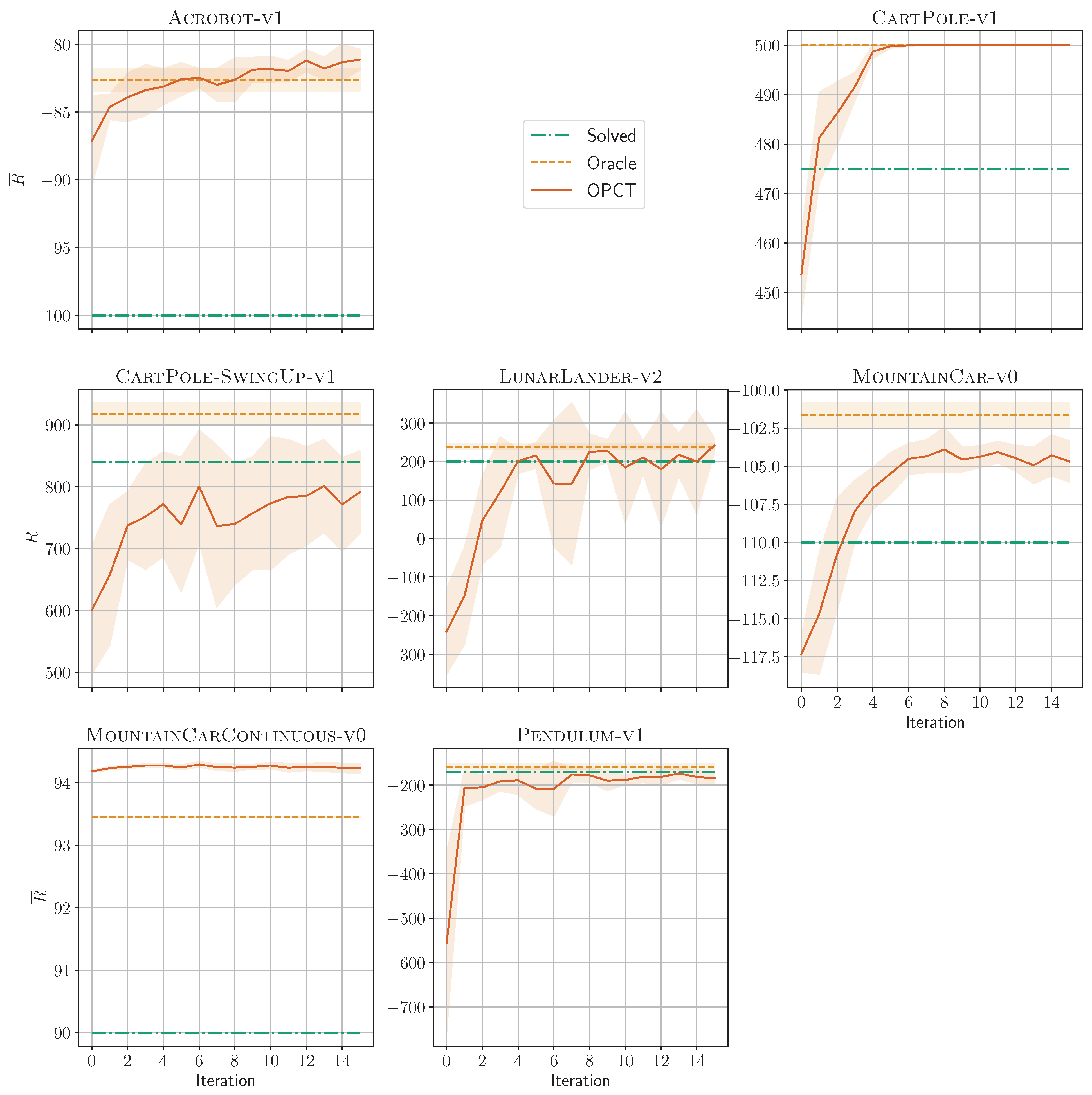
4.1. Solving Environments

Figure 2 shows our main result: For all environments and all presented algorithms, we plot the return R ¯ as a function of DT depth d. ITER usually reaches the solved-threshold (dash-dotted green line) at lower depths than the other two algorithms. It is the only one to solve all investigated environments (at depths up to 10). For each environment, we select one of the successful DRL agents (see Table 2).
Table 2a shows these results in compact quantitative form: which is the minimum depth needed to reach the solved-threshold of an environment? (Note that these numbers can be deceptive; a 10 + might be from a tree being below the threshold only by a tiny margin or a 5 might hide the fact that a depth-4 tree is only slightly below the threshold.) As can be seen, ITER outperforms the other algorithms. Its sum of depths is roughly half of the other algorithms’ sums. Depth ( 1 ) for MountainCarContinuous + BB has been put in brackets because it is somewhat unstable. At depths 2 and 3 the performance is below the threshold, as can be seen from Figure 2. Additionally, Table 2 shows algorithms EPS and ITER for CART as baseline experiments. In both cases, CART does not reach the performance of OPCT, at least not for shallow depths.
Figure 2 shows another remarkable result: DTs can often even surpass the performance of the DRL agents they originate from (the oracles, dashed orange lines). In Table 2b, we report the minimum depths at which DT performances exceeds the oracle’s performance. While these numbers can be deceptive too (CartPole-SwingUp + ITER almost reaches oracle performance at depth 8), they show that there is not necessarily a trade-off between model complexity and performance. DTs require orders of magnitude fewer parameters (see Section 4.4.1) and can exhibit higher performance. Again, ITER is the best-performing algorithm in this respect. In Section 4.3 and Section 5, we discuss why such a performance better than the oracle’s can occur.
Figure 3 and Figure 4 demonstrate the evolution of OPCT performance in algorithm ITER. The first iterations provide samples in new regions of the observation space (Figure 3, as compared to the regions visited by the oracle) and they are marked by a sharp increase in performance R ¯ (Figure 4).

4.2. Computational Complexity

The algorithms presented here differ significantly in computing time, as shown in Table 3. All experiments were performed on a CPU device (i7-10700K 8 × 3.8 GHz). To ensure methodological consistency, we let each algorithm generate the same total number of samples, namely n s = 30,000.
In every algorithm, we average over 10 trees for each depth d = 1 , , 10 due to fluctuations, and to represent the time needed in t O P C T . Additionally, ITER performs I m a x + 1 iterations for all depths. Hence, a single run takes 10 · t O P C T time for both EPS and BB while taking 10 · ( I m a x + 1 ) · t O P C T time for ITER. (Here, the time t O P C T reflects the performance of an algorithm in the particular environment, depending on whether more or less time is required for a desired result.) However, the most time-consuming part of a run is the evaluation of the trees, i.e., the generation of samples by running 100 evaluation episodes in the environment. According to these observations, ITER takes the most time to complete.

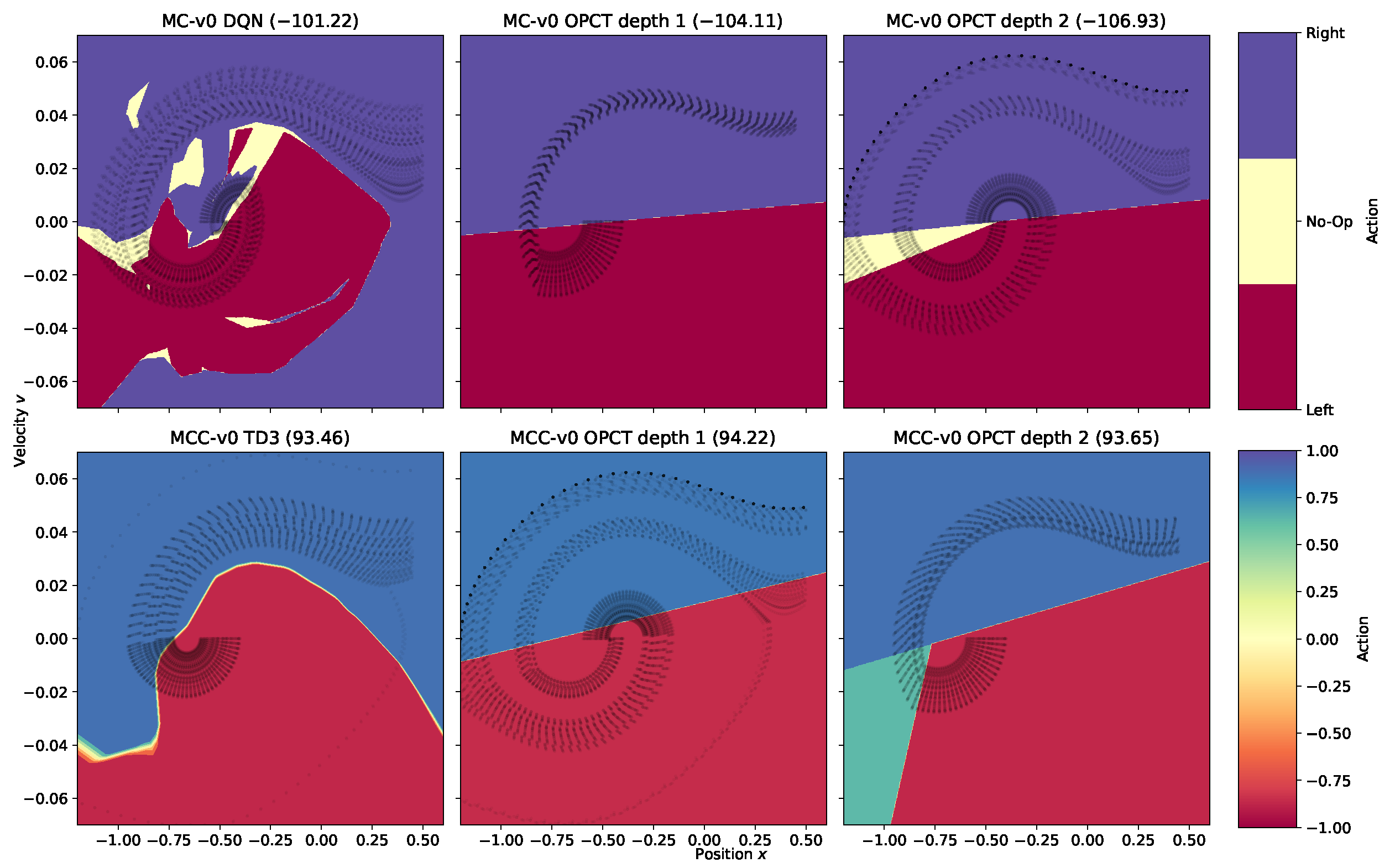
4.3. Decision Space Analysis

Two-dimensional observation spaces offer the possibility of visual inspection of the agents’ decision-making. This can provide additional insights and offer explanations of bad results in certain settings. Figure 5 shows the decision surfaces of DRL agents and OPCTs for MountainCar in the discrete (top row) and continuous (bottom row) versions. DRL agents can often learn a needlessly complicated partitioning of the observation space, as can be seen prominently in the top left plot, e.g., by yellow patches of “no-acceleration” in the upper left or the blue “accelerate right” area in the bottom right, which are never visited by oracle episodes. This poses a problem for the BB algorithm because it samples, e.g., from the blue bottom right area and therefore, DTs learn in part “wrong” actions, resulting in poor performance. Thus, the inspection of the oracle’s decision space reveals the reason for the partial failure of the BB algorithm in the case of MountainCar at low depths.
On the other hand, algorithm ITER will not be trained with samples from regions never visited by oracle or tree episodes. Hence, it has no problem with the blue bottom right area. It delivers more straightforward rules at depth d = 1 or d = 2 (shown in columns 2 and 3 of Figure 5), and yields returns slightly better than the oracle because it generalizes better given its fewer degrees of freedom.

4.4. Explainability for Oblique Decision Trees in RL

Explainability is significantly more difficult to achieve for agents operating in environments with multiple time steps than in those with single time steps (by “single time step” we mean that a decision follows directly in response to a single input record, e.g., classification or regression). This is because the RL agent has to execute a possibly long sequence of action decisions before collecting the final return (also known as the credit assignment problem [30,31]).
Given their simple, transparent nature, DTs offer interesting options for explainability in such environments with multiple time steps, which are not immediately applicable to opaque DRL models. This section will illustrate steps towards explainability in RL through shallow DTs.

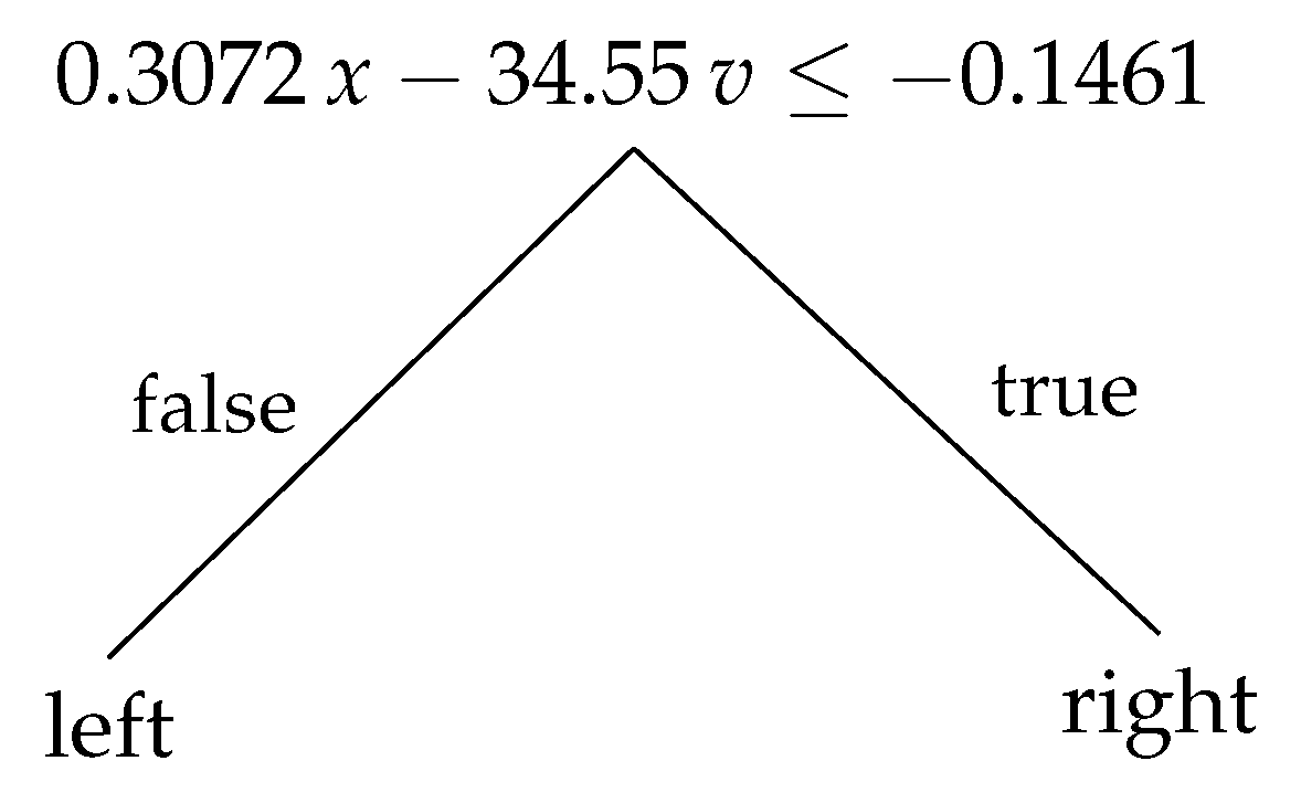
4.4.1. Decision Trees: Compact and Readable Models

Trees are useful for XAI since they are usually much more compact than DRL models and consist of a set of explicit rules, which are simple in that they are linear inequalities in the input features (for oblique DTs). As an example of the models’ simplicity, Figure 6 shows a very compact OPCT of depth 1 for the MountainCar challenge. On the other hand, DRL models have many trainable parameters and form complex, nonlinear features from the input observations. Table 4 shows the number of trainable weights for all our SB3 oracles (DRL models) which are, in all cases, orders of magnitude larger than the number of trainable tree parameters.
The number of parameters in the oracle can be computed from the architecture of the respective policy network. For example, in MountainCar with input dimension D = 2 , the DQN consists of 2 networks: a Q- and a target network. Each has D + 1 = 2 + 1 inputs (including bias), 3 action outputs, and a ( 256 , 256 ) hidden layer architecture (we do not use overly complex DRL architectures but keep the default parameters suggested by the SB3 methods [26]), which results in
2 · ( 2 + 1 ) · 256 + ( 256 + 1 ) · 256 + 256 · 3 = 134 , 656   weights .
The number of parameters in the tree is a function of the tree’s depth and the input dimension. For example, in LunarLander with input dimension D = 8 , the oblique tree of depth d = 2 (as obtained by, e.g., ITER) has 2 d 1 = 3 = 1 + 2 split nodes and 2 d = 4  leaf nodes. Each split node has D + 1 = 9 parameters (one weight for each input dimension + threshold), and each leaf node has one adjustable output parameter (the action), resulting in
3 · 9 + 4 = 31   parameters .
However, it should be emphasized that all our DTs have been trained with the guidance of a DRL oracle. At least so far, we could not find a procedure to construct successful DTs solely from interaction with the environment. Such direct tree learning is left for future work. In this paper, we rely on the guidance of the oracle, whose samples demonstrate reasonable solutions to the tree and facilitate learning.
In a sense, the DT “explains” the oracle by offering a simpler surrogate action model. The surrogate is often nearly as good as or even better than the DRL model in terms of mean reward.
It is a surprising result of our investigations that trees of small depth delivering such high rewards could be found at all. Most prominently, for the environments Acrobot and LunarLander with their higher input dimensions 6 and 8, it was not expected beforehand to find successful trees of depth 1 and 2, respectively.

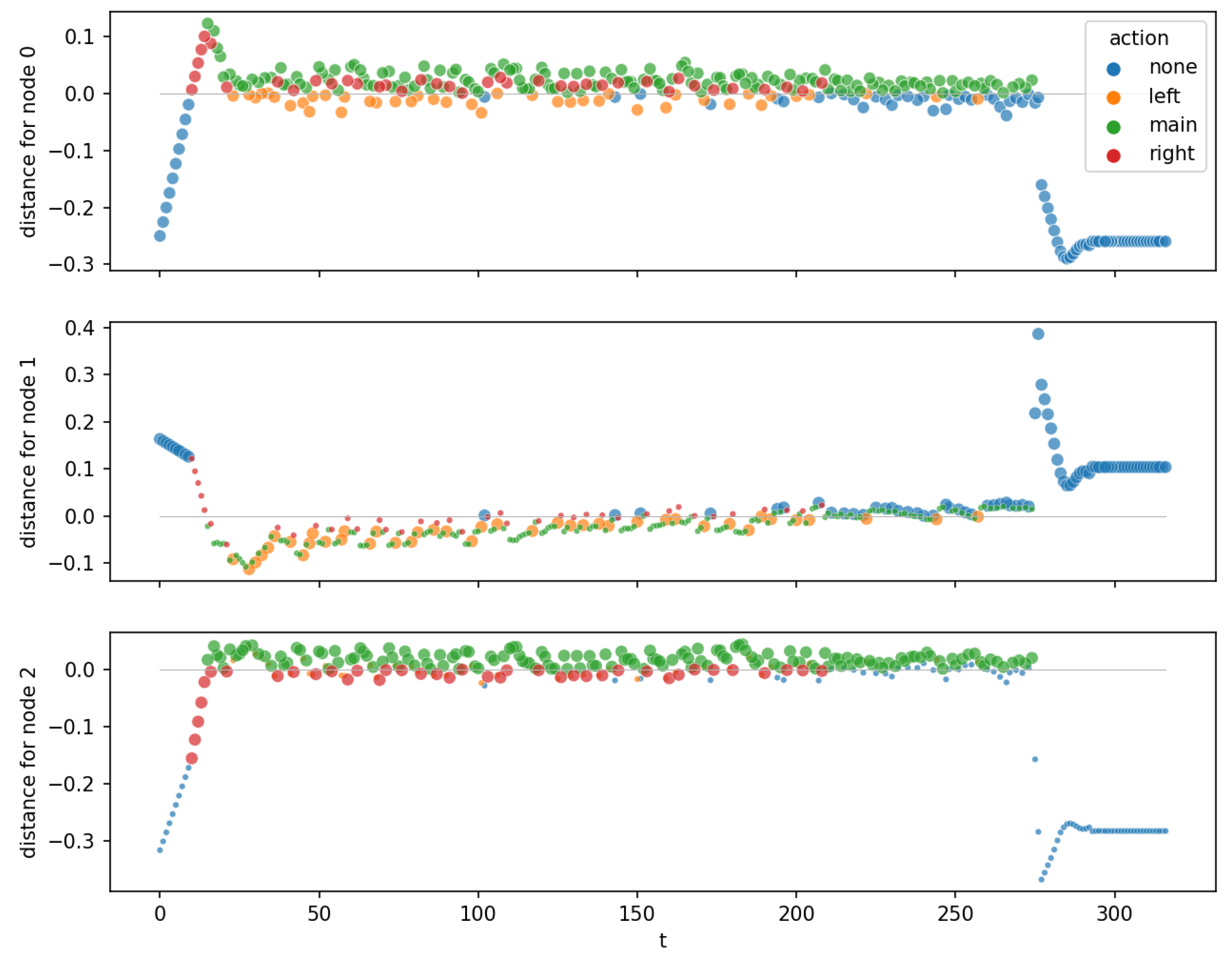
4.4.2. Distance to Hyperplanes

Further insights that help to explain a DT can be gained by visualizing the distance to hyperplanes of the nodes of a DT. According to Equation (1), each split node has an associated hyperplane in the observation space so that observations above or below this hyperplane take a route to different subtrees (or leaves) of this node.
Although hyperplanes in higher dimensions are difficult to visualize and interpret, the distance to each hyperplane is easy to visualize, regardless of the dimension of the observation space. It can be shown that even an anisotropic scaling of the observation space leaves the relations between all distances to a particular hyperplane intact, i.e., they are changed only by a common factor (see Appendix B).
Figure 7 shows the distance plots for the three nodes 0 , 1 , 2 of the ITER OPCT for LunarLander. A distance plot shows the distances of the observations to the node’s hyperplane for a specific episode as a function of time step t. Each observation is colored by the action the DT has taken. It is seen in Figure 7 that after a short transient period ( t 40 ), the distances for every node stay small while the lander sinks. At about time step t 280 , the lander touches the ground and the distances increase (because all velocities are forced to be zero, all positions and angles are forced to certain values prescribed by the shape of the ground), which is, however, irrelevant for the control of the lander and the success of the episode. All nodes are attracting nodes (points are attracted to the respective hyperplane), which bring the ship to an equilibrium (a sinking position with constant v y ) that guarantees a safe landing.
Another example is shown in Figure 8 for the three nodes 0 , 1 , 2 of the ITER OPCT for Pendulum. These are the three upper nodes of a tree with depth 3 and, therefore, seven split nodes. Node 0 is an attracting one (“equilibrium node”) because the distances approach zero (here: for t 64 ). Nodes 1 and 2 do not exhibit a zero distance in the equilibrium state; instead, they are “swing-up nodes” responsible for bringing energy into the system through appropriate action switching.
The lower left plot (“distance to equilibrium”) of Figure 8 shows the distance of each observation to the unstable equilibrium point ( cos θ , sin θ , ω ) = ( 1 , 0 , 0 ) (the desired goal state). Interestingly, at  t = 64 (vertical gray line), where the distance to node 0 is already close to zero, the distance to the equilibrium point is not yet zero (but soon will be). This is because the hyperplane is oriented in such a way that for small angle θ , the angular velocity ω is approximately ω = 5.3 sin ( θ ) (read off from the node’s parameters). The hyperplane tells us on which path the pole approaches the equilibrium point. The control strategy is to raise ω for points below the hyperplane and to lower ω for points above. This amounts to the fact that a tilted pole obtains an ω (corresponding to a certain kinetic energy) such that the pole will come to rest at θ = 0 . The exact physical equation requires that the kinetic energy has the same value as the necessary change in potential energy,
E k i n ( ω ) = Δ E p o t ( θ ) 1 6 m l 2 ω 2 = m g 2 m g 2 cos ( θ ) ,
leading to the angular velocity
ω = 3 g 2 ( 1 cos θ ) 5.5 sin ( θ / 2 ) ( for   g = 10 , = 1 )
which is not too far from the control strategy found by the node.
Similar patterns (equilibrium nodes + swing-up nodes) can be observed in those environments where the goal is to reach or maintain certain (unstable) equilibrium points (CartPole-SwingUp, CartPole). Environments like MountainCar(Continuous) or Acrobot, which do not have an equilibrium state as goal, consist only of swing-up nodes as shown in Figure 9 for Acrobot.
In summary, the distance plots show us two characterizing classes of nodes:
  • Equilibrium nodes (or attracting nodes): nodes with distance near to zero for all observation points after a transient period. These nodes occur only in those environments where an equilibrium has to be reached.
  • Swing-up nodes: nodes that do not stabilize at a distance close to zero. These nodes are responsible for swing-up, for bringing energy into a system. The trees for environments MountainCar, MountainCarContinuous, and Acrobot consist only of swing-up nodes because, in these environments, the goal state to reach is not an equilibrium.

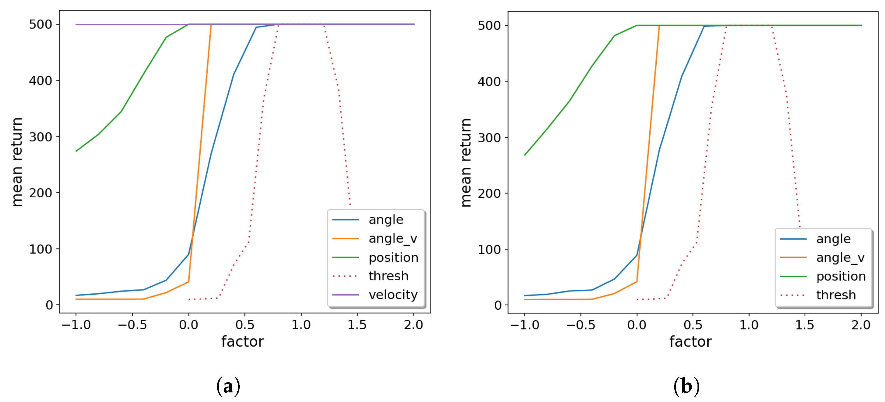
4.4.3. Sensitivity Analysis

An individual rule of an oblique tree is simple in mathematical terms (it is a linear inequality). It is, nevertheless, difficult to interpret for humans. This is because the individual input features (usually different physical quantities) are multiplied with weights and added up, which has no direct physical interpretation.
For example, the single-node tree of CartPole has the rule
4.904 x 0.1829 v s . + 19.1497 θ + 1.5203 ω 0.0003
w x x + w v v s . + w θ θ + w ω ω τ
which does not directly tell which input features are important for success and is as such difficult to interpret. However, due to the simple mathematical relationship, we may vary each weight w i or the threshold τ individually and measure the effect on the reward. This is shown in Figure 10. The weights are varied in a wide range of [ 100 % , 200 % ] of their nominal value, the threshold τ (being close to 0) is varied in the range τ w ¯ + [ 0 % , 200 % ] · w ¯ , where w ¯ is the mean of all weight magnitudes | w i | of the node.
From Figure 10a, we learn that the angle θ is the most important input feature. If w θ is below its nominal value, performance starts to degrade, while a higher w θ keeps the optimal reward. The most important parameter is the threshold τ , which has to be close to 0; otherwise, performance quickly degrades on both sides. This makes sense because the essential control strategy for the CartPole is to react to slightly positive or negative θ with the opposite action.
On the other hand, the weight for velocity v is the least important parameter; varying it in Figure 10a does not change the reward, and setting its weight w v to 0 and varying the other weights leads to essentially the same picture in Figure 10b.
One could object that these sensitivity analyses results could have also been read off directly from Equation (2) because θ has the largest, and v has the most negligible weight in magnitude. However, this is only an accidental coincidence. For many other nodes that we examined using sensitivity analysis, the most/least important feature in terms of mean return did not coincide with the largest/smallest weight.
Suppose an OPCT has more than one node, e.g., for LunarLander at depth d = 2 with its three split nodes. In that case, we can perform a sensitivity analysis for each node separately, or vary the respective weights and thresholds for all nodes simultaneously. The latter is shown in Figure 11. We see that strengthening their weights (setting them to higher values than nominal ones) only leads to slow degradation for all input features. A faster degradation occurs when lowering the weight for a certain input feature. The features v y , θ , and  v x (in this order) are the most important in that respect. On the other hand, the legs (boolean variables signaling the ground-contact of the lander’s legs), are least important. The curves in Figure 11b only change slightly if the legs are removed from the decisions by setting their weights to zero. This makes sense because the legs have a constant no-contact value during the majority of episode steps (and when the legs do reach ground-contact, the success or failure of an episode is usually already determined).
Note that the sensitivity analysis shown here is, in a sense, more detailed than a Shapley value analysis [32] because it allows us to disentangle the effects of intensifying or weakening an input feature. In contrast, the Shapley value only compares the presence or absence of a feature. (It is of course also less detailed, because it does not take coalitions of features into account as Shapley does.) It is also computationally less intensive; measuring the Shapley value for RL problems by computing the mean reward over many environment episodes and many coalitions would be, in most cases, prohibitively time-consuming.
Our sensitivity analysis has some similarity to the layer-wise relevance propagation (LRP) investigated by Bach, Montavon, and others [33,34]. LRP has been developed in particular for (deep) neural networks, but the concept of input feature relevance is similar.

5. Discussion

For a broader perspective, we want to point out a number of issues related to our findings.
  • To align our work in the context of XAI, we may use the guidance of the taxonomy proposed by (Schwalbe and Finzel [35], Section 5):
    • The problem definition: The task consists of a classification or regression (for discrete or continuous actions, respectively) of tabular, numerical data (observations). We intend a post hoc explanation of DRL oracles, by finding decision trees described that are inherently transparent and simulatable in that a human can follow the simple mathematical and hierarchical structure of a DT’s decision-making process.
    • Our algorithm as an explanator requires a model (the oracle and also the environment’s dynamics) as input, while still being portable by not relying on a specific type of oracle. The output data of our algorithm are shallow DTs as surrogate models mimicking the decision-making process of the DRL oracles. This leads to a drastic reduction of model parameters (see Table 4). Given their simple and transparent nature, DTs lend themselves to rule-based output and to further explanations by example or by counterfactuals, and analysis of feature importance (as we showed in Section 4.4.3).
    • As the fundamental functionally grounded metric of our algorithm, we compare the DT’s average return in the RL environment with the oracle’s performance. This measures the fidelity to the oracle in the regions relevant to successfully solve the environment and the accuracy with respect to the original task of the environment. We do not evaluate human-grounded metrics. (Human-grounded metrics are defined by Schwalbe and Finzel [35] as metrics involving human judgment of the explainability of the constructed explanator (here: DT): how easy is it for humans to build a mental model of the DT, how accurately does the mental model approximate the explanator model, and so on.) Instead, we trust that the simple structure and mathematical expressions used in the DTs generated by our algorithms, as well as the massively reduced number of model parameters, lead to an interpretability and effectiveness of predictions that could not be achieved with DRL models. In Section 4.4, we have explained aspects connected to this in more detail.
  • Can we understand why the combination ITER + OPCT is successful, while the combination EPS + OPCT is not? We have no direct proof, but from the experiments conducted, we can share these insights: Firstly, equilibrium problems such as CartPole or Pendulum exhibit a severe oversampling of some states (i.e., the upright pendulum state). If, as a consequence, the initial DT is not well-performing, ITER allows to add the correct oracle actions for problematic samples and to improve the tree in critical regions of the observation space. Secondly, for environment Pendulum we observed that the initial DT was “bad” because it learned only from near-perfect oracle episodes. It had not seen any samples outside the near-perfect episode region and hypothesized the wrong actions in the outside regions (see Figure 3). Again, ITER helps; a “bad” DT is likely to visit these outside regions and then add samples combined with the correct oracle actions to its sample set.
    We conclude that algorithm ITER is successful because it strikes the right balance between being too exploratory, like algorithm BB (which might sample from constraint-violating regions or from regions unknown to the oracle), and not exploratory enough, like algorithm EPS (which might sample only from the narrow region of successful oracle trajectories). Algorithm ITER solves the sampling challenges mentioned in Section 1. It works well based on its iterative nature, which results in self-correction of the tree. At every iteration, the trajectories generated by the tree form a dataset of state–action pairs. The oracle corrects the wrong actions, and the tree can improve its behavior based on the enlarged dataset.
  • We investigated another possible variant of an iterative algorithm. In this variant, observations were sampled while the oracle was training (and probably also visited unfavorable regions of the observation space). After the oracle had completed its training, the samples were labeled with the action predictions of the fully trained oracle. These labeled samples were presented to DTs in a similar iterative algorithm as described above. However, this algorithm was not successful.
  • A striking feature of our results is that DTs (predominantly those trained with ITER) can outperform the oracle they were trained from. This seems paradoxical at first glance, but the decision space analysis for MountainCar in Section 4.3 has shown the likely reason. In Figure 5, the decision spaces of the oracles are overly complex (similar to overfitted classification boundaries, although overfitted is not the proper term in the RL context). With their significantly reduced degrees of freedom, the DTs provide simpler, better generalizing models. Since they do not follow the “mistakes” of the overly complex DRL models, they exhibit a better performance. It fits to this picture that the MountainCarContinuous results in Figure 2 are best at d = 1 (better than oracle) and slowly degrade towards the oracle performance as d increases; the DT obtains more degrees of freedom and mimics the (slightly) non-optimal oracle better and better. The fact that DTs can be better than the DRL model they were trained on is compatible with the reasoning of Rudin [20], who stated that transparent models are not only easier to explain but often also outperform black box models.
  • We applied algorithm ITER to OPCTs. Can CARTs also benefit from ITER? The solved-depths shown in column ITER + CART of Table 2a add up to 35 + , which is nearly as bad as EPS + CART ( 38 + ). Only the solved-depth for Pendulum improved somewhat from 10 + to 7. We conclude that the expressive power of OPCTs is important for being successful in creating shallow DTs with ITER.
  • What are the limitations of our algorithms? In principle, the three algorithms EPS, BB, and ITER are widely applicable since they are model-agnostic concerning the DRL and DT methods used and applicable to any RL environment. However, the limitation of the current work is that, so far, we have only tested environments with one-dimensional action spaces (discrete or continuous). There is no principled reason why the algorithms should not be applicable to multi-dimensional action spaces (OPCTs can be trained for multi-dimensional outputs as well). Still, the empirical demonstration of successful operation in multi-dimensional action spaces is a topic for future work. One obvious limitation of the three algorithms is that they need a working oracle. A less obvious limitation is that algorithm EPS only needs static, pre-collected samples from oracle episodes (in other applications, these might be “historical” samples). In contrast, the algorithms BB and ITER really need an oracle function to query for the right action at arbitrary points in the observation space. Which points are needed is not known until the algorithms BB and ITER are run.
  • A last point worth mentioning is the intrinsic trustworthiness of DTs. They partition the observation space in a finite (and often small) set of regions, where the decision is the same for all points. (This feature includes smooth extrapolation to yet-unknown regions.) DRL models, on the other hand, may have arbitrarily complex decision spaces. If such a model predicts action a for point x, it is not known which points in the neighborhood of x will have the same action.

6. Conclusions

In this article we have shown that a considerable range of classic control RL problems can be solved with DTs. Even higher-dimensional problems (Acrobot and LunarLander) can be solved with surprisingly simple trees. We have presented three algorithms for generating training data for DTs. The training data are composed of the RL environment’s observations and the corresponding DRL oracle’s decisions.
These algorithms differ in the way the points of the observation space are selected. In EPS, all samples visited by the oracle during evaluation episodes are used, BB means that random samples from a hyperrectangle in the observation space are taken, while ITER is an algorithm that takes points in the observation space visited by previous iterations of trained DTs. Our experiments show how DTs derived with these algorithms can generally not only solve the challenges posed by classic control problems at very moderate depths but also reach or even surpass the performance of the oracle. ITER produces good results on all tested environments with equal or lower DT depths than the other two algorithms. Furthermore, we discuss the advantages of transparent DT models with very few parameters, especially compared to DRL networks, and show how they allow to gain insights that would otherwise be hidden by opaque DRL decision-making processes.
However, our algorithms still require DRL agents as a prerequisite for creating successful DTs.
Future work should test our algorithms on increasingly complex RL environments. ITER still requires fine-tuning of parameters, such as the number of base samples and number of samples per iteration, to optimize sample efficiency and performance.
Our work is intended to provide helpful arguments for simple, transparent RL agents and to advance the knowledge in the field of explainable RL.

Author Contributions

Conceptualization, R.C.E., M.L., L.W. and W.K.; investigation, R.C.E., M.O. and W.K.; methodology, R.C.E., M.O., M.L., L.W. and W.K., project administration, R.C.E., M.O. and W.K.; software, R.C.E., M.O. and W.K.; supervision, L.W. and W.K.; validation, R.C.E., M.O. and W.K.; visualization, R.C.E., M.O. and W.K.; writing—original draft, R.C.E., M.O. and W.K.; writing—review & editing, R.C.E., M.O., M.L., L.W. and W.K. All authors have read and agreed to the published version of the manuscript.

Funding

This research was supported by the research training group “Dataninja” (Trustworthy AI for Seamless Problem Solving: Next Generation Intelligence Joins Robust Data Analysis) funded by the German federal state of North Rhine-Westphalia.

Data Availability Statement

The experiments presented in this article are openly available in our Github repository https://github.com/MarcOedingen/Iterative-Oblique-Decision-Trees (accessed on 25 May 2023).

Conflicts of Interest

The authors declare no conflict of interest. The funders had no role in the design of the study; in the collection, analyses, or interpretation of data; in the writing of the manuscript; or in the decision to publish the results.

Appendix A. Reproduction of PIRL via NDPS Results

Verma et al. [13] provide policies found by their method for the classic control problems Acrobot, CartPole (in the shorter version v0), and MountainCar in ([13], Appendix B, Figures 8–10) as well as returns obtained by optimal policies found by two versions of their algorithm in rows Ndps-SMT and Ndps-BOPT of ([13], Appendix A, Table 6). We implemented the provided policies in Python and evaluated them on 100 episodes in each respective environment. (In the case of MountainCar, there must have been a typographic error as the reported policy produced the lowest possible return of R ¯ = 200 ± 0 . Therefore, we switched the actions, leading to the results reported below).
As shown in Table A1, our results differ from the reported ones for two of the three environments. Compatible results could only be reproduced for Acrobot.
Table A1. Results of two versions of NDPS (SMT and BOPT) as published in [13], and the average return R ¯ and standard deviation of our implementations of the reported policies in 100 episodes.
Verma et al. [13]Our Reproduction
Environment R ¯ SMT , R ¯ BOPT R ¯ ± σ R ¯ solved
Acrobot-v1 0 84.16 , 127.21 −93.29 ± 25.19 100
CartPole-v0 183.15 , 143.21 46.66 ± 15.34 195
MountainCar-v0 108.06 , 143.86 −163.02 ± 3.48 110

Appendix B. Effect of Observation Space Normalization on the Distances to Hyperplane

In a D-dimensional observation space every point is given by x = ( x 1 , x 2 , , x D ) . Every decision hyperplane is defined by
x · w = x 1 · w 1 + x 2 · w 2 + + x D · w D = b
with weight vector w T = ( w 1 , w 2 , , w D ) and bias b.
The distance d of a point x to a given hyperplane is computed by
d = | i = 1 D x i · w i b | i = 1 D w i 2
Now we perform an anisotropic scaling of the observables by subtracting a dimension-specific constant μ i and by dividing with another dimension-specific constant σ i for i = 1 , 2 , , D :
x i = x i μ i σ i
The hyperplane in the scaled space is defined by
x · w = b
Substituting (A3) in (A4) leads to
x 1 μ 1 σ 1 · w 1 + x 2 μ 2 σ 2 · w 2 + + x n μ D σ D · w D = b
x 1 w 1 σ 1 μ 1 σ 1 w 1 + x 2 w 2 σ 2 μ 2 σ 2 w 2 + + x D w D σ D μ D σ D w D = b
Comparison of coefficients with (A1) results in
w i = w i σ i
b = b + i = 1 D μ i σ i w i
or, respectively,
w i = w i · σ i
b = b i = 1 D μ i σ i w i σ i = b i = 1 D μ i w i
The distance in the scaled space is
d = | i = 1 D x i · w i b | i = 1 D w i 2
Substituting (A3), (A9), and (A10)
d = | i = 1 D x i μ i σ i · w i σ i b + i = 1 D μ i w i | i = 1 D ( w i σ i ) 2
= | i = 1 D ( x i μ i ) w i b + i = 1 D μ i w i | i = 1 D ( w i σ i ) 2
= | i = 1 D ( x i w i μ i w i ) b + i = 1 D μ i w i | i = 1 D ( w i σ i ) 2
= | i = 1 D x i w i i = 1 D μ i w i b + i = 1 D μ i w i | i = 1 D ( w i σ i ) 2
= | i = 1 D x i w i b | i = 1 D ( w i σ i ) 2
Finally a comparison with (A2) results in
d = d i = 1 D w i 2 i = 1 D ( w i σ i ) 2 = d i = 1 D w i 2 i = 1 D w i 2 = d | | w | | | | w | |
Thus, we have shown that anisotropic scaling changes the distances of all points to a given hyperplane only by a common factor (unlike point-to-point distances, which usually change by different factors depending on the direction of the vector connecting these points).

Abbreviations

The following abbreviations are used in this manuscript:
BBBounding Box algorithm
CARTClassification and Regression Trees
DRLDeep Reinforcement Learning
DQNDeep Q-Network
DTDecision Tree
EPSEpisode Samples algorithm
ITERIterative Training of Explainable RL models
OPCTOblique Predictive Clustering Tree
PPOProximal Policy Optimization
RLReinforcement Learning
SB3Stable-Baselines3
TD3Twin Delayed Deep Deterministic Policy Gradient

References

  1. Engelhardt, R.C.; Lange, M.; Wiskott, L.; Konen, W. Sample-Based Rule Extraction for Explainable Reinforcement Learning. In Proceedings of the Machine Learning, Optimization, and Data Science, Certosa di Pontignano, Italy, 18–22 September 2022; Nicosia, G., Ojha, V., La Malfa, E., La Malfa, G., Pardalos, P., Fatta, G.D., Giuffrida, G., Umeton, R., Eds.; Springer: Cham, Switzerland, 2023; Volume 13810, pp. 330–345. [Google Scholar] [CrossRef]
  2. Adadi, A.; Berrada, M. Peeking inside the black-box: A survey on explainable artificial intelligence (XAI). IEEE Access 2018, 6, 52138–52160. [Google Scholar] [CrossRef]
  3. Molnar, C.; Casalicchio, G.; Bischl, B. Interpretable Machine Learning—A Brief History, State-of-the-Art and Challenges. In Proceedings of the ECML PKDD 2020 Workshops, Ghent, Belgium, 14–18 September 2020; Koprinska, I., Kamp, M., Appice, A., Loglisci, C., Antonie, L., Zimmermann, A., Guidotti, R., Özgöbek, Ö., Ribeiro, R.P., Gavaldà, R., Eds.; Springer: Cham, Switzerland, 2020; pp. 417–431. [Google Scholar] [CrossRef]
  4. Molnar, C. Interpretable Machine Learning: A Guide for Making Black Box Models Explainable. 2022. Available online: https://christophm.github.io/interpretable-ml-book (accessed on 25 May 2023).
  5. Puiutta, E.; Veith, E.M.S.P. Explainable Reinforcement Learning: A Survey. In Proceedings of the Machine Learning and Knowledge Extraction, Dublin, Ireland, 25–28 August 2020; Holzinger, A., Kieseberg, P., Tjoa, A.M., Weippl, E., Eds.; Springer: Cham, Switzerland, 2020; pp. 77–95. [Google Scholar] [CrossRef]
  6. Heuillet, A.; Couthouis, F.; Díaz-Rodríguez, N. Explainability in deep reinforcement learning. Knowl.-Based Syst. 2021, 214, 106685. [Google Scholar] [CrossRef]
  7. Milani, S.; Topin, N.; Veloso, M.; Fang, F. A survey of explainable reinforcement learning. arXiv 2022, arXiv:2202.08434. [Google Scholar] [CrossRef]
  8. Lundberg, S.M.; Erion, G.; Chen, H.; DeGrave, A.; Prutkin, J.M.; Nair, B.; Katz, R.; Himmelfarb, J.; Bansal, N.; Lee, S.I. From local explanations to global understanding with explainable AI for trees. Nat. Mach. Intell. 2020, 2, 56–67. [Google Scholar] [CrossRef] [PubMed]
  9. Liu, G.; Schulte, O.; Zhu, W.; Li, Q. Toward Interpretable Deep Reinforcement Learning with Linear Model U-Trees. In Proceedings of the Machine Learning and Knowledge Discovery in Databases, Dublin, Ireland, 10–14 September 2018; Berlingerio, M., Bonchi, F., Gärtner, T., Hurley, N., Ifrim, G., Eds.; Springer: Cham, Switzerland, 2019; Volume 11052, pp. 414–429. [Google Scholar] [CrossRef] [Green Version]
  10. Mania, H.; Guy, A.; Recht, B. Simple random search of static linear policies is competitive for reinforcement learning. In Advances in Neural Information Processing Systems; Bengio, S., Wallach, H., Larochelle, H., Grauman, K., Cesa-Bianchi, N., Garnett, R., Eds.; Curran Associates, Inc.: New York, NY, USA, 2018; Volume 31. [Google Scholar]
  11. Coppens, Y.; Efthymiadis, K.; Lenaerts, T.; Nowé, A.; Miller, T.; Weber, R.; Magazzeni, D. Distilling deep reinforcement learning policies in soft decision trees. In Proceedings of the IJCAI 2019 Workshop on Explainable Artificial Intelligence, Macao, China, 10–16 August 2019; pp. 1–6. [Google Scholar]
  12. Frosst, N.; Hinton, G.E. Distilling a Neural Network Into a Soft Decision Tree. In Proceedings of the First International Workshop on Comprehensibility and Explanation in AI and ML, Bari, Italy, 16–17 November 2017. [Google Scholar]
  13. Verma, A.; Murali, V.; Singh, R.; Kohli, P.; Chaudhuri, S. Programmatically Interpretable Reinforcement Learning. In Proceedings of the 35th International Conference on Machine Learning, Stockholm, Sweden, 10–15 July 2018; Proceedings of Machine Learning Research; Dy, J., Krause, A., Eds.; PMLR: New York, NY, USA, 2018; Volume 80, pp. 5045–5054. [Google Scholar]
  14. Qiu, W.; Zhu, H. Programmatic Reinforcement Learning without Oracles. In Proceedings of the Tenth International Conference on Learning Representations, ICLR, Virtual, 25–29 April 2022. [Google Scholar]
  15. Ross, S.; Gordon, G.; Bagnell, D. A Reduction of Imitation Learning and Structured Prediction to No-Regret Online Learning. In Proceedings of the Fourteenth International Conference on Artificial Intelligence and Statistics, Ft. Lauderdale, FL, USA, 11–13 April 2011; Proceedings of Machine Learning Research; Gordon, G., Dunson, D., Dudík, M., Eds.; PMLR: New York, NY, USA, 2011; Volume 15, pp. 627–635. [Google Scholar]
  16. Bastani, O.; Pu, Y.; Solar-Lezama, A. Verifiable Reinforcement Learning via Policy Extraction. In Advances in Neural Information Processing Systems; Bengio, S., Wallach, H., Larochelle, H., Grauman, K., Cesa-Bianchi, N., Garnett, R., Eds.; Curran Associates, Inc.: New York, NY, USA, 2018; Volume 31. [Google Scholar]
  17. Zilke, J.R.; Loza Mencía, E.; Janssen, F. DeepRED—Rule Extraction from Deep Neural Networks. In Proceedings of the Discovery Science, Bari, Italy, 19–21 October 2016; Calders, T., Ceci, M., Malerba, D., Eds.; Springer: Cham, Switzerland, 2016; Volume 9956, pp. 457–473. [Google Scholar] [CrossRef]
  18. Schapire, R.E. The strength of weak learnability. Mach. Learn. 1990, 5, 197–227. [Google Scholar] [CrossRef] [Green Version]
  19. Freund, Y.; Schapire, R.E. A Decision-Theoretic Generalization of On-Line Learning and an Application to Boosting. J. Comput. Syst. Sci. 1997, 55, 119–139. [Google Scholar] [CrossRef] [Green Version]
  20. Rudin, C. Stop explaining black box machine learning models for high stakes decisions and use interpretable models instead. Nat. Mach. Intell. 2019, 1, 206–215. [Google Scholar] [CrossRef] [PubMed] [Green Version]
  21. Brockman, G.; Cheung, V.; Pettersson, L.; Schneider, J.; Schulman, J.; Tang, J.; Zaremba, W. OpenAI Gym. arXiv 2016, arXiv:1606.01540. [Google Scholar] [CrossRef]
  22. Lovatto, A.G. CartPole Swingup—A Simple, Continuous-Control Environment for OpenAI Gym. 2021. Available online: https://github.com/0xangelo/gym-cartpole-swingup (accessed on 25 May 2023).
  23. Schulman, J.; Wolski, F.; Dhariwal, P.; Radford, A.; Klimov, O. Proximal Policy Optimization Algorithms. arXiv 2017, arXiv:1707.06347. [Google Scholar] [CrossRef]
  24. Mnih, V.; Kavukcuoglu, K.; Silver, D.; Graves, A.; Antonoglou, I.; Wierstra, D.; Riedmiller, M. Playing Atari with Deep Reinforcement Learning. arXiv 2013, arXiv:1312.5602. [Google Scholar] [CrossRef]
  25. Fujimoto, S.; van Hoof, H.; Meger, D. Addressing Function Approximation Error in Actor-Critic Methods. In Proceedings of the 35th International Conference on Machine Learning, Stockholm, Sweden, 10–15 July 2018; Proceedings of Machine Learning Research; Dy, J., Krause, A., Eds.; PMLR: New York, NY, USA, 2018; Volume 80, pp. 1587–1596. [Google Scholar]
  26. Raffin, A.; Hill, A.; Gleave, A.; Kanervisto, A.; Ernestus, M.; Dormann, N. Stable-Baselines3: Reliable Reinforcement Learning Implementations. J. Mach. Learn. Res. 2021, 22, 12348–12355. [Google Scholar]
  27. Breiman, L.; Friedman, J.H.; Olshen, R.A.; Stone, C.J. Classification And Regression Trees; Routledge: New York, NY, USA, 1984. [Google Scholar]
  28. Pedregosa, F.; Varoquaux, G.; Gramfort, A.; Michel, V.; Thirion, B.; Grisel, O.; Blondel, M.; Prettenhofer, P.; Weiss, R.; Dubourg, V.; et al. Scikit-learn: Machine Learning in Python. J. Mach. Learn. Res. 2011, 12, 2825–2830. [Google Scholar]
  29. Stepišnik, T.; Kocev, D. Oblique predictive clustering trees. Knowl.-Based Syst. 2021, 227, 107228. [Google Scholar] [CrossRef]
  30. Alipov, V.; Simmons-Edler, R.; Putintsev, N.; Kalinin, P.; Vetrov, D. Towards practical credit assignment for deep reinforcement learning. arXiv 2021, arXiv:2106.04499. [Google Scholar] [CrossRef]
  31. Woergoetter, F.; Porr, B. Reinforcement learning. Scholarpedia 2008, 3, 1448. [Google Scholar] [CrossRef]
  32. Roth, A.E. (Ed.) The Shapley Value: Essays in Honor of Lloyd S. Shapley; Cambridge University Press: Cambridge, UK, 1988. [Google Scholar] [CrossRef]
  33. Bach, S.; Binder, A.; Montavon, G.; Klauschen, F.; Müller, K.R.; Samek, W. On pixel-wise explanations for non-linear classifier decisions by layer-wise relevance propagation. PLoS ONE 2015, 10, e0130140. [Google Scholar] [CrossRef] [Green Version]
  34. Montavon, G.; Binder, A.; Lapuschkin, S.; Samek, W.; Müller, K.R. Layer-Wise Relevance Propagation: An Overview. In Explainable AI: Interpreting, Explaining and Visualizing Deep Learning; Samek, W., Montavon, G., Vedaldi, A., Hansen, L.K., Müller, K.R., Eds.; Springer: Cham, Switzerland, 2019; pp. 193–209. [Google Scholar] [CrossRef]
  35. Schwalbe, G.; Finzel, B. A comprehensive taxonomy for explainable artificial intelligence: A systematic survey of surveys on methods and concepts. Data Min. Knowl. Discov. 2023, 1–59. [Google Scholar] [CrossRef]
Figure 1. Flowchart of ITER (Algorithm 1).
Algorithms 16 00282 g001
Figure 2. Return R ¯ as a function of DT depth d for all environments and all presented algorithms. The solved-threshold is shown as dash-dotted green line, the average oracle performance as dashed orange line, and the DTs performances as solid lines with average and ± 1 σ of ten repetitions as shaded area. Note: (i) For Acrobot we show two plots to include the BB curve. (ii) Good performance in CartPole leads to overlapping curves: oracle, BB, and ITER are all constantly at R ¯ = 500 .
Algorithms 16 00282 g002
Figure 3. Evolution of the training dataset with iterations for OPCT of depth 5 for Pendulum (observables mapped back to 2D). The plots show from left to right the observations added to the dataset in each iteration (by the oracle in iteration 0 and by the tree in iterations 1–3).
Algorithms 16 00282 g003
Figure 4. Evolution of OPCT performance with iterations. Shown are mean ± 1 σ of 10 repetitions. Generally, the return increases notably in the first few iterations. For most environments, a significant improvement after 10 iterations is not observed. (The OPCTs’ depths are chosen according to Table 2a.)
Algorithms 16 00282 g004
Figure 5. Decision surfaces for MountainCar (MC, discrete actions) and MountainCarContinuous (MCC, continuous actions). Column 1 shows the DRL agents. The OPCTs in column 2 (depth 1) and column 3 (depth 2) were trained with algorithm ITER. The number in brackets in each subplot title is the average return R ¯ . The black dots represent trajectories of 100 evaluation episodes with same starting conditions across the different agents. They indicate the regions actually visited in the observation space.
Algorithms 16 00282 g005
Figure 6. OPCT of depth 1 obtained by ITER solving MountainCar with a return of R ¯ = 107.47 in 100 evaluation episodes.
Algorithms 16 00282 g006
Figure 7. Distance to hyperplanes for LunarLander. The diagrams show root node, left child, and right child from top to bottom. Small points: node is “inactive” for this observation (the observation is not routed through this node). Big points: node is “active”.
Algorithms 16 00282 g007
Figure 8. Distance plots for Pendulum. Three of the diagrams show the distance to the hyperplanes of root node 0, left child node 1, and right child node 2. The lower left plot shows the distance to the equilibrium point ( 1 , 0 , 0 ) in observation space. The vertical line at t = 64 marks the step where the distance for node 0 approaches zero.
Algorithms 16 00282 g008
Figure 9. Distance plot for Acrobot. The tree has only one node.
Algorithms 16 00282 g009
Figure 10. OPCT sensitivity analysis for CartPole: (a) including all weights, (b) with velocity weight w v set to zero. Parameter angle is the most important, velocity is least important.
Algorithms 16 00282 g010
Figure 11. OPCT sensitivity analysis for LunarLander: (a) including all weights, (b) with the weights for the legs set to zero. v y is most important, the ground-contacts of the legs are least important.
Algorithms 16 00282 g011
Table 1. Overview of environments used. A task is considered solved when the average return in 100 evaluation episodes is R s o l v e d . Environments with an undefined official threshold R s o l v e d have been assigned a reasonable one. This number is then reported in parenthesis.
EnvironmentObservation Space ( O )Action Space ( A ) R solved
Acrobot-v1First angle cos ( θ 1 ) [ 1 , 1 ] ,
First angle sin ( θ 1 ) [ 1 , 1 ] ,
Second angle cos ( θ 2 ) [ 1 , 1 ] ,
Second angle sin ( θ 2 ) [ 1 , 1 ] ,
Angular velocity θ 1 ˙ = ω 1 [ 4 π , 4 π ] ,
Angular velocity θ 2 ˙ = ω 2 [ 9 π , 9 π ]
a Apply torque{-1 (0),
0 (1),
1 (2)}
100
CartPole-v1Position cart x [ 4.8 , 4.8 ] ,
Velocity cart v ( , ) ,
Angle pole θ [ 0.42 , 0.42 ] ,
Velocity pole ω ( , )
a Accelerate{left (0),
right (1)}
475
CartPole-
SwingUp-v1
Position cart x [ 2.4 , 2.4 ] ,
Velocity cart v ( , ) ,
Angle pole cos ( θ ) [ 1 , 1 ] ,
Angle pole sin ( θ ) [ 1 , 1 ] ,
Angular velocity pole ω ( , )
a Accelerate{left (0),
not (1),
right (2)}
undef.
( 840 )
LunarLander-v2Position x [ 1.5 , 1.5 ] ,
Position y [ 1.5 , 1.5 ] ,
Velocity v x [ 5 , 5 ] ,
Velocity v y [ 5 , 5 ] ,
Angle θ [ π , π ] ,
Angular velocity θ ˙ = ω [ 5 , 5 ] ,
Contact center leg l l { 0 , 1 } ,
Contact right leg l r { 0 , 1 }
a Fire{not (0),
left engine (1),
main engine (2),
right engine (3)}
200
MountainCar-v0Position x [ 1.2 , 0.6 ] ,
Velocity v [ 0.07 , 0.07 ]
a Accelerate{left (0),
not (1),
right (2)}
110
MountainCar
Continuous-v0
Same as MountainCar-v0 a Accelerate [ 1 , 1 ] 90
Pendulum-v1Angle cos ( θ ) [ 1 , 1 ] ,
Angle sin ( θ ) [ 1 , 1 ] ,
Angular velocity ω [ 8 , 8 ]
a Apply torque [ 2 , 2 ] undef.
( 170 )
Table 2. The numbers show the minimum depth of the respective algorithm for (a) solving an environment and (b) surpassing the oracle. ( ) + means no DT of investigated depths could reach the threshold. See main text for explanation of (1) or (3). Bold numbers mark the best result(s) in each row.
(a) Solving an environment
Algorithms
EPSEPSBBITERITER
EnvironmentModelCARTOPCTOPCTCARTOPCT
Acrobot-v1DQN11 10 + 11
CartPole-v1PPO33131
CartPole-SwingUp-v1DQN10 + 10 + 10 + 10 + 7
LunarLander-v2PPO10 + 10 + 210 + 2
MountainCar-v0DQN33531
MountainCarContinuous-v0TD311(1)11
Pendulum-v1TD310 + 9675
Sum38 + 37 + 35 + 35 + 18
(b) Surpassing the oracle
Acrobot-v1DQN33 10 + 21
CartPole-v1PPO561(3)1
CartPole-SwingUp-v1DQN 10 + 10 + 10 + 10 + 10 +
LunarLander-v2PPO 10 + 10 + 2 10 + 3
MountainCar-v0DQN35634
MountainCarContinuous-v0TD3 10 + 1421
Pendulum-v1TD3 10 + 98106
Sum 51 + 44 + 41 + 40 + 26 +
Table 3. Computation times of our algorithms for some environments (we selected those with different observation space dimensions D). Shown are the averaged results from 10 runs. t r u n : average time elapsed for one run covering all depths d = 1 , , 10 . t O P C T : average time elapsed to train and evaluate 10 OPCTs. n s : total number of samples used. Note how the bad performance of BB in the Acrobot environment leads to longer episodes and therefore longer evaluation times t O P C T .
Environmentdim DAlgorithm t run [ s ] t OPCT [ s ] n s
Acrobot-v16EPS124.82 ± 1.9611.71 ± 0.9530,000
BB477.70 ± 7.8947.56 ± 2.9230,000
ITER1189.14 ± 28.7010.76 ± 1.0230,000
CartPole-v14EPS187.39 ± 3.6418.06 ± 2.2930,000
BB202.65 ± 1.2619.11 ± 1.1330,000
ITER2040.16 ± 21.4618.50 ± 1.6430,000
MountainCar-v02EPS85.39 ± 1.507.93 ± 0.5730,000
BB104.92 ± 2.0510.27 ± 0.5430,000
ITER849.90 ± 19.797.68 ± 0.6130,000
Table 4. Oracle and tree complexity. (D denotes the dimension of the observation space).
Number of Parameters
EnvironmentDim DModelOracleITERDepth d
Acrobot-v16DQN136,71091
CartPole-v14PPO915571
CartPole-SwingUp-v15DQN534,5348907
LunarLander-v28PPO9797312
MountainCar-v02DQN134,65651
MountainCarContinuous-v02TD3732,40651
Pendulum-v13TD3734,8061565
Disclaimer/Publisher’s Note: The statements, opinions and data contained in all publications are solely those of the individual author(s) and contributor(s) and not of MDPI and/or the editor(s). MDPI and/or the editor(s) disclaim responsibility for any injury to people or property resulting from any ideas, methods, instructions or products referred to in the content.

