Article

JointContrast: Skeleton-Based Interaction Recognition with New Representation and Contrastive Learning †

1
School of Software, North University of China, Taiyuan 030051, China
2
College of Computer Science and Technology, Nanjing University of Aeronautics and Astronautics, Nanjing 210016, China
3
Research Center for Big Data Intelligence, Zhejiang Lab., Hanghzou 310058, China
4
School of Computer and Information, Anhui Normal University, Wuhu 241000, China
5
School of Computer Science and Engineering, Anhui University of Science and Technology, Huainan 232001, China
*
Authors to whom correspondence should be addressed.
Extension of the paper published in the 19th Pacific Rim International Conference on Artificial Intelligence (PRICAI’22), Shanghai, China, 10–13 November 2022.
Algorithms 2023, 16(4), 190; https://doi.org/10.3390/a16040190
Submission received: 16 February 2023 / Revised: 21 March 2023 / Accepted: 21 March 2023 / Published: 30 March 2023
(This article belongs to the Special Issue Machine Learning in Pattern Recognition)

Abstract

:
Skeleton-based action recognition depends on skeleton sequences to detect categories of human actions. In skeleton-based action recognition, the recognition of action scenes with more than one subject is named as interaction recognition. Different from the single-subject action recognition methods, interaction recognition requires an explicit representation of the interaction information between subjects. Recalling the success of skeletal graph representation and graph convolution in modeling the spatial structural information of skeletal data, we consider whether we can embed the inter-subject interaction information into the skeletal graph and use graph convolution for a unified feature representation. In this paper, we propose the interaction information embedding skeleton graph representation (IE-Graph) and use the graph convolution operation to represent the intra-subject spatial structure information and inter-subject interaction information in a uniform manner. Inspired by recent pre-training methods in 2D vision, we propose unsupervised pre-training methods for skeletal data as well as contrast loss. In SBU datasets, JointContrast achieves 98.2 % recognition accuracy. in NTU60 datasets, JointContrast respectively achieves 94.1 % and 96.8 % recognition accuracy under Cross-Subject and Cross-View evaluation metrics.

1. Introduction

Action recognition detects a number of predefined human action categories and has a wide range of applications, including video surveillance, human-computer interaction and sports health. Various kinds of data are available for action recognition, such as RGB video, depth map sequences, and skeleton data. Compared to other kinds of data, skeletal data is insensitive to changes in appearance, background, and perspective, which records the motion trajectory of certain joints [1,2,3]. In skeleton-based action recognition, the recognition of action scenes with multi-subjects is named as interaction recognition, and it is observed that many scenes in the study are mutual actions, such as handshakes, hugs, etc. While there are a large number of generic methods available for skeleton-based action recognition, it is not the case for interaction recognition, where there are considerably fewer methods and studies. Additionally, recent research [4,5,6,7,8,9] has revealed that generic action recognition methods are not always effective for interaction recognition tasks. These generic recognition methods for interaction recognition can be categorized into two groups: (1) using only the primary subject of the skeleton data for spatial information representation, and (2) utilizing all subjects of the skeleton data for feature representation, with feature fusion performed at a certain stage. However, these methods cannot produce accurate feature representations for interaction recognition because: (1) mutual action involves more than one key subject, and the interaction information between the key subjects must be explicitly represented, and (2) the spatial structure of intra-subject joints is influenced by inter-subject interaction, hence the spatial structure and interaction information should be represented in a unified manner. Previous studies defined the spatial structure information in skeletal data as dependencies between joints, but in a multi-subject scenario, dependencies between inter-subject joints should be defined as interaction information. Recalling the success of skeletal graph representation and graph convolution in modeling the spatial structural information of skeletal data, we propose the interaction information embedding graph representation (IE-Graph) and use the graph convolution to represent the intra-subject spatial structure information and inter-subject interaction information in a uniform manner. In contrast to the skeleton graph where only joint-adjacent edges exist, we incorporate subject-adjacent edges in the proposed IE-Graph to represent the interaction information between subjects.
In addition, inspired by recent pre-training methods in 2D vision, we propose unsupervised pre-training methods for skeletal data. As we all known, the representation learning is one of the main driving forces of deep learning research. Pre-trained on a rich source dataset, the model is able to learn generalized and useful weight parameters for downstream tasks. After fine-tuning on the target dataset, the model can obtain performance gains on specific tasks. The success of pre-training in natural language processing [10,11] and computer vision [12,13,14,15] has proven its effectiveness and advancement. Especially when the pre-training phase is unsupervised, it is possible to utilize a practically infinite train set size in pre-training. However, training from scratch on the target dataset is still the dominant approach in skeleton-based tasks. The aim of this work is to advance the representation of skeletal data through the study of unsupervised pre-training. To this end, we propose an unsupervised pre-training framework for skeletal data, as well as a contrastive loss for the pre-training pretext task. The proposed contrastive loss uses the features of corresponding joints from different viewpoints as contrast elements to learn more generalized weight parameters by backward propagation.
We validate our method on the SBU and NTU RGB-D datasets and the experimental results demonstrate the effectiveness of the method. In addition, we demonstrate whether the proposed IE-Graph and pre-training framework enhance the performance of the model and whether they can be applied to other methods through ablation experiments. Our contributions can be summarized as follows:
  • We propose an innovative interaction information embedding graph representation (IE-Graph), which represents interaction information as subject-adjacent edges and helps in the representation of interaction and better feature fusion;
  • With the help of IE-Graph, the model can use graph convolution to represent the intra-subject spatial information and inter-subject interaction information in a uniform manner, which allows us to generalize the single-subject action recognition methods to interaction recognition easily;
  • We propose a contrastive loss as well as an unsupervised pre-training framework for skeletal data;
  • We perform experiments on three popular benchmarks, including SUB, NTU60, and NTU120, and the results show that JointContrast achieves competitive results in comparison with several popular baseline methods.

2. Related Works

2.1. Skeleton-Based Action Recognition

Different from the grid structure data, e.g., RGB iamge and video, the skeleton data has an irregular structure. Generally, the 3D skeletal data is converted to pseudo-images in order to meet the needs of CNN based methods [2,16]. It is necessary to carefully design the joint traversal so that the CNN model can learn the dependencies between joints, however, this is not easy. As an extension of convolution on graph structure, graph convolution networks (GCN) have been successfully applied to skeletal data. The GCN-based method extracts the human body as a skeleton graph, where the joints are the nodes, and the bones are the edges. During the graph convolution operation, each node first constructs the set of neighboring nodes by joint-adjacent edges, and then updates its own feature representation by learning the dependencies with the joints in the neighboring set. With the stacking of GCNs, each node has a larger receptive field and learns the dependencies with more nodes. ST-GCN [17] proposes a spatial-temporal graph to represent the skeleton data. Intra-subject and inter-frame edges respectively link body joints and the same joints between consecutive frames, which model the spatial and temporal information. then the model based on GCN learn spatial-temporal features and co-occurrence between them. Previous approaches relied on hand-crafted traversal rules to reflect the dependencies between joints, which is limited in terms of performance and generality. Li, M. et al. [18] identify inconsistencies between latent dependencies and physical connections between joints, for which this work proposes a data-driven approach to construct skeleton maps to represent action-specific latent dependencies. Recently, The success of Transformer in natural language processing and vision tasks has led to widespread interest in self-attentive mechanisms. Attention-based methods have been successfully applied to skeletal data tasks and learn latent dependencies between joints more efficiently. DEST-Net [19] introduces a attention block for adaptive modeling spatial and temporal dependencies between joints, which does not require manual design of joint traversal rules. KA-AGTN [20] models the spatial dependencies between joints by the multi-head self-attention, and the proposed Temporal Kernel Attention (TKA) block generates a channel-level attention score using temporal features to enhance temporal motion correlation. However, self-attentive-based models are difficult to train because it takes a long time for attention to move from the global to a specific few points.

2.2. Interaction Recognition

Early works [21,22,23,24,25] on interaction recognition is based on hand-crafted features. Yun, K. et al. [22] utilize joints relation of inter-subject, intra-subject, inter-frames and intra-frames as feature representation, and then feed them to SVM for recognition. Li, M. et al. [26] propose a novel graph model to encode class-specific person–person interaction patterns in each single-view case and then combine the features of each single-view case for interaction recognition. Recent works [6,9,27,28,29,30,31] focus on deep learning. M. et al. [4] introduce Relational Network (RN) for interaction recognition, which utilize pair-wise joints as input to learn the relationship information of joint pairs. Yang. et al. [5] enhances the action recognition mothod ST-GCN so that it can represent the interaction information between multiple subjects to solve the interaction recognition problem.

2.3. Contrastive Learning

Because of its great unsupervised potential, Contrastive learning [15,32,33] has attracted the attention of many researchers. The essence of contrastive learning is to maximize the similarity of representations between positive samples while encouraging the discrimination of negative samples [34]. Recent works [35,36] have also utilized contrastive learning for unsupervised representation learning and pre-training. However, in skeleton-based tasks, scratch training over the target dataset is still the dominant approach .

3. Methods

3.1. Preliminaries

Deep learning methods have been used to model and represent graph data. Traditional neural networks are limited to processing Euclidean data. By using representational learning, graph neural networks have generalized deep learning models to show good performance on structured graph data [37]. Graph neural network (GNN) models have been shown to be a powerful family of networks that learn representations by aggregating features of entities and neighbors [38], The extension of neural networks to data with graph structures is a new topic in deep learning research, and the application of convolutional and recurrent neural networks to graph is widely mentioned. Graph Convolutional Network (GCN), as an extension of convolutional neural networks to graph structures, is a general and effective framework for learning graph-structured data representations. In skeletal data action recognition, the human body is considered as a hinge system consisting of joints and bones and is represented as a skeletal graph. We use G t = ( V t , A t ) to denote the skeleton data at t frame, where V t = { V t i } i = 1 N represents the set of all N joints and A t represents the joint-adjacency edges set. Define the neighboring set of V t i as N ( V t i ) = { V t j | d ( V t i , V t j ) D } , where d ( V t i , V t j ) is the shortest path distance from V t i to V t j . In addition, A predefined labelling function l : V t { 1 , 2 , , k } sets the label { 1 , 2 , , K } for each node V t i V t in the graph, which divides the neighboring set N ( V t i ) into a fixed number of K subsets. The graph convolution is calculated in the form of
Y ( V t i ) = V t i N ( V t i ) 1 Z t i ( V t i ) X ( V t j ) W ( l ( V t j ) )
where X ( V t j ) denotes the feature representation of node V t j , W ( · ) is the weight parameters assigned by the weight function according to the label of each node. Z t i ( V t i ) is the number of elements in the subset where the node is located, which is used to normalize the feature representation. The representation of V t i after the graph convolution is denoted as Y ( V t i ) . Using the adjacency matrix, the Equation (1) can be expressed as:
Y ( V t i ) = k = 1 K Λ k 1 2 A k Λ k 1 2 X W k
where A k is the adjacency matrix formed by the nodes labeled k { 1 , 2 , , K } in the spatial configuration and λ k i i = j A k i j is the degree matrix of the adjacency matrix.
In our work, we partition the neighboring sets of nodes based on the shortest path distance between them, which is similar to the relative distance used in convolutional neural networks. The partition function can be expressed as l t i ( V t j ) = d ( V t i , V t j ) . When the neighbouring set is defined as the shortest path less than 2, it is possible to give a matrix representation of each subset after partitioning in a simpler way, such as [17]. In this paper, we give how to generate the adjacency matrix representation of the partitioned subsets under arbitrary distance settings. We define the polynomial of the adjacency matrix A t as ϕ k ( A t ) , where k is the number of highest terms. When k = 0 , we have ϕ k ( A t ) = I for the unit matrix, indicating that the neighboring nodes of each joint are only itself; when k = 1 , we have ϕ k ( A t ) = A t indicating that the neighboring nodes of each joint are constructed according to the body structure A t . It is important to note that in a single-subject action scene, A t is represented by the adjacency matrix of the skeletal graph constructed by only one subject, but in our work, we focus on scenes with multi-subjects actions, so A t represents the adjacency edges of multiple independent skeletal graphs constructed by multiple subjects in one frame. When the highest number of polynomials k > 2 , according to the definition of the distance partitioning strategy we have
[ Φ k ( A ) ] i , j = 1 i f d i s t ( V t i , V t j ) = k 0 e l s e
Equation (3) shows that we have [ Φ k ( A ) ] i , j = 1 only if the shortest path distance between V t i and V t j is equal to k, where i , j denote the row and column coordinates of the matrix, respectively. When k > 2 , we can compute the value of each position in the matrix Φ k ( A ) by traversing all nodes, but the time complexity of doing so is quadratic. Recall the meaning of multiplying adjacency matrices, i.e., each element in A t k represents the number of paths from i to j that pass through exactly k edges. To this end, we can obtain Φ k ( A t ) by A t k and Φ j ( A t ) , j < k :
Φ k ( A t ) = I , i f k = 0 A t , i f k = 1 I ( A t k I ( i = 0 k 1 ϕ i ( A t ) ) ) , e l s e
where I ( x ) is a function whose output is zero or one:
I ( x ) = 0 , i f x = 0 1 , e l s e
The partitioning strategy based on distance can avoid dividing the same points into different subsets, while the partitioning strategy has a hierarchical structure that can learn finer-grained local features and learn the dependencies between nodes at longer distances as the network deepens, which is consistent with the idea and practice of convolutional neural networks.

3.2. Interaction Embedding Graph

Because graph convolution is used for spatial domain feature extraction, a predefined graph structure for the graph convolution is required, and the traditional graph structure cannot meet the requirements of accurate interaction recognition for modeling interaction information. Since only the coordinates of joints are used as known data in the skeletal data, the interaction between subjects can be understood as a feature representation of the implicit relationship between different subject joints. While graph convolution can model the relationship between joints within a single subject, it can also model interaction information. The problem is that multiple subjects form multiple independently connected graphs, but information cannot be propagated between them, which is why single-subject action recognition methods cannot achieve superior performance in interaction recognition.
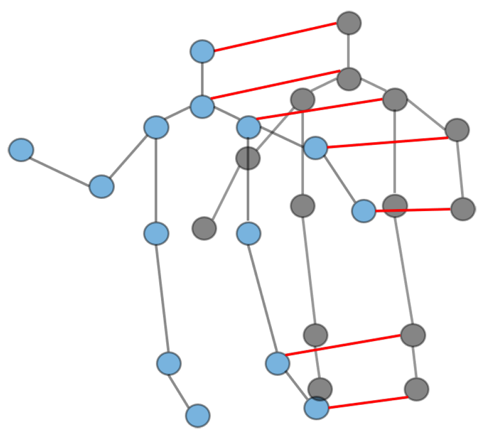
First we need to construct a graph representation of each subject, which is the same as the traditional skeleton graph representation, except that there are multiple subjects in the scene, and secondly, we introduce another kind of edge to model the interaction information. To distinguish between these two kinds of edges, we call the naturally connected edge within a subject a joint edge—which connects neighboring joints within the same subject—and call the other kind of edge that connects the same joints between different subjects a subject edge. As shown in Figure 1, we use blue and black nodes to represent the joints of the different subjects, and the corresponding colored edges to represent the joint edges within the different subjects. In addition, we use subject edges to connect the skeleton graphs of different subject constructions. For brevity, we do not label all subject edges in the figure. Intuitively, the subject edge converts the independent skeletal graphs composed of multiple subjects into a unified connected graph, which enables modeling of interaction information and feature fusion between multiple subjects after graph convolution; Objectively, the addition of subject edges increases the number of neighbors of each joint, and as mentioned above, the increase of neighbors in the graph convolution means the increase of the receptive field, which means that each joint can not only learn the feature representation within the same subject, but also obtain useful information from other subjects.
Because joint edges and subject edges are discriminatively constructed for modeling spatial structure features and interaction features, we use two different adjacency matrices for separate representations. We also use A t R M N to denote the adjacency matrix composed of joint edges, where M and N are the number of subjects and the number of joints per subject, respectively. In general, the joints of each target labeled by the dataset are the same, so A t is a diagonal matrix consisting of the joint adjacency matrix of each subject. In addition, we use the adjacency matrix B t R M N to store our predefined subject edges. Another reason we use two matrices for separate representations is that we use two different matrices of learnable parameters in the network to model joint and subject edges separately, one for learning spatial information and the other for interaction information. However, pre-defined subject edges are not sufficient, as they are less helpful for modeling relationships between joints at longer distances. Inspired by the edge-learnable weight matrix in graph convolution, we propose the subject edge-learnable matrix B , which has the same dimension size as B t . Any graph convolution operation performed with a predefined subject edge B T is accompanied by a B to learn the relational representation between distant joints. With the addition of predefined target edges and dynamic subject edges, the graph convolution operation also needs to be changed accordingly to complete the representation of the interaction information features, and the improved graph convolution can be expressed as:
Y ( V t i ) = 1 K 1 k = 0 k 1 1 D k 1 ϕ k ( A t ) X t W k + 1 K 2 k = 1 K 2 1 D k ϕ k ( B t ) X t W k
Equation (6) adds a new term to the Equation (2), which completes the modeling of the interaction information. K 2 is similar to K 1 as a hyperparameter controlling the neighbouring set of each node defined by the subject edge. D k is the degree matrix of Φ k ( B t , A t ) , which serves to perform normalization of the features by eliminating the influence of the number of neighboring joints on the output, which can be calculated by [ D k ] i j = j ( [ Φ k ( B t , A t ) ] i j ) . W k R C × C is a matrix of learnable parameters formed by superimposing the weight vectors of multiple output channels, where C and C represent the input and output feature dimensions, respectively. Similar to the definition of Φ k ( A t ) , we define ϕ k ( B t , A t ) as a polynomial of the adjacency matrix B t and A t .
ϕ [ k ] ( B t , A t ) = B t , i f k = 1 I ( B t A t k 1 I ( i = 1 k 1 ϕ i ( B t , A t ) ) )
The definition of I ( x ) is the same as its definition in Φ k ( A t ) . In the neighborhood defined by the joint edges, we use a distance partitioning strategy to partition the neighboring joints into K 1 subsets, and use the learnable weights W k in each subset to model the influence of the joints in each subset on the central joint to update the features so that it aggregates structural information from the other joints. We also partition the neighboring joints defined by the subject edges into K 2 subsets according to the distance partitioning strategy, and model the influence of the joints in each subset on the centroid using the learnable weights W k , but in this case the graph convolution operation models the interaction information between the subjects. While it is possible to simply increase K 2 to make distant joints also neighbors of the central node, there are several drawbacks to such an approach: (1) increased receptive fields increase the model memory and inference time cost; (2) excessively large K 2 can result in loops that make the model represent redundant joint dependencies. Therefore, we introduce a data-driven dynamic subject edge. In the implementation, we represent it as a learnable matrix B with the same dimensions as B t , accompanied by B t at each occurrence of ϕ [ k ] ( B t , A t ) and denoted as ϕ [ k ] ( B t , A t ) + B . Note that B is shared in each graph convolution operation and is initialized to an all-zero matrix.

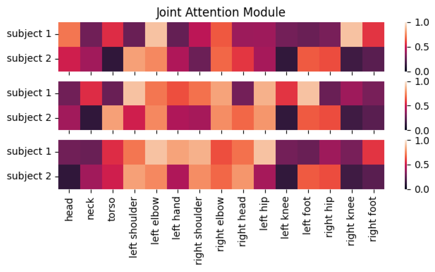
3.3. Joint Attention Module

Most graph convolution methods use graph representations to represent skeletal data and model the relationships between joints using learnable weights in the networks. However, there is no network or operation that can be used to enhance key joint features throughout the process. We thus introduce an attention mechanism. Unlike previous work [39] that introduced attention weights in graph convolutional networks, our JAM has three distinct advantages: (1) the module is designed independently of the backbone network, so it can be used by other backbone networks; (2) the independently designed JAM utilizes both temporal and spatial domain information, and these spatio-temporal features can help it learn more robust attention weights; (3) with the feature map of the whole skeletal sequence as input, the module can learn the importance of each joint in a global view.
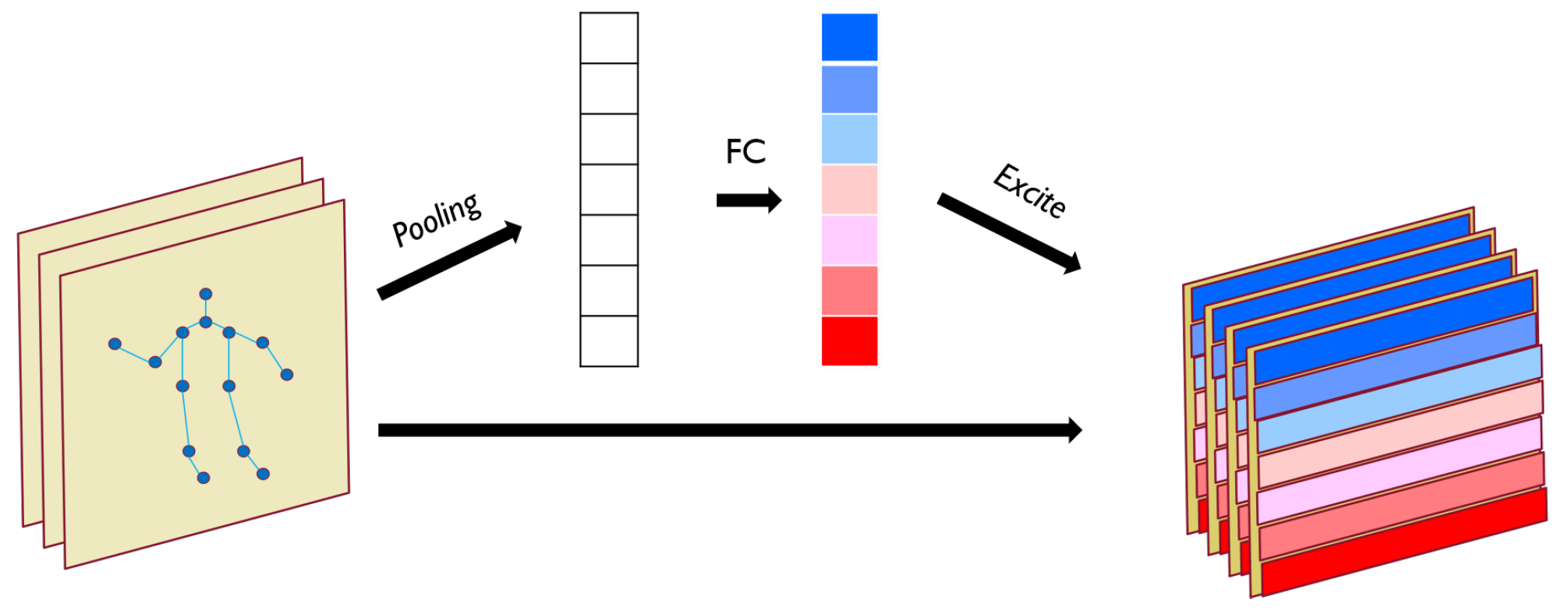
The JAM learns from the spatio-temporal information feature map output from the previous layer and arranges different attention weights for different joints. As shown in Figure 2, for a given input feature map with dimensions ( C , N , T ) , the entire feature map first undergoes a pooling operation, which generates a joint description feature map by aggregating the feature maps in the temporal dimension. The role of joint description feature map is to generate embeddings corresponding to the global distribution of each joint feature, allowing the global information from the network to be used by later network layers. Following the feature aggregation is the excitation, which takes the global distribution embedding as input to generate modulation weights for each joint. These weights are then applied to the original input feature map to produce the output of the entire JAM.
Specifically, the JAM is a computational unit that maps the input X R C × N × T to the feature map X R C × N × T . We define X = { x 1 , , x N } , where x i R C × T is the feature representation corresponding to the joint i. The signal in each output feature map is obtained by a locality operation, so that each cell of the transformed output feature map cannot make use of information from the context outside that region. Therefore, we use a pooling operation to convert the input features associated with the global temporal domain into a joint description feature map, which is achieved by performing a global average pooling. Formally, the joint description feature map Z = z 1 , , z 2 is generated by collapsing the temporal dimension T. For example, the description feature z i R C of the i joint is computed as follows
z i = 1 T t = 1 T x i [ : , j ]
To take advantage of the information aggregated in the pooling operation, we follow the activation operation with the aim of obtaining joint attention weights. To achieve this target, the activation operation must satisfy two requirements: (1) it must be flexible enough to learn nonlinear interactions between joints, and (2) it needs to learn non-reciprocal relationships, since we want to allow the existence of multiple key joints, rather than emphasizing only one of them. Therefore, we select to use a gated network with a S i g m o i d activation function.
s = σ ( W 2 δ ( W 1 z ) )
where σ and δ are the S i g m o i d and R e L U activation functions, respectively, W 1 R C a × C , W 2 R 2 × C a . To limit the size and complexity of the JAM, we implement the gate mechanism through a bottleneck structure that consists of two fully connected strata and two nonlinear activation functions. The number of channels of the middle-state feature map in the bottleneck structure is determined by the scaling factor a, and then the feature dimension is reduced to 1 by the R e L U activation function and the fully-connected layer. The final output of JAM is the modulated feature map.
X ^ = s X
where the dimension of X ^ is the same as X . The JAM can be integrated into our backbone network. In addition, the flexibility of the block means that it can be applied to other networks.

3.4. Pre-Training and Contrastive Loss

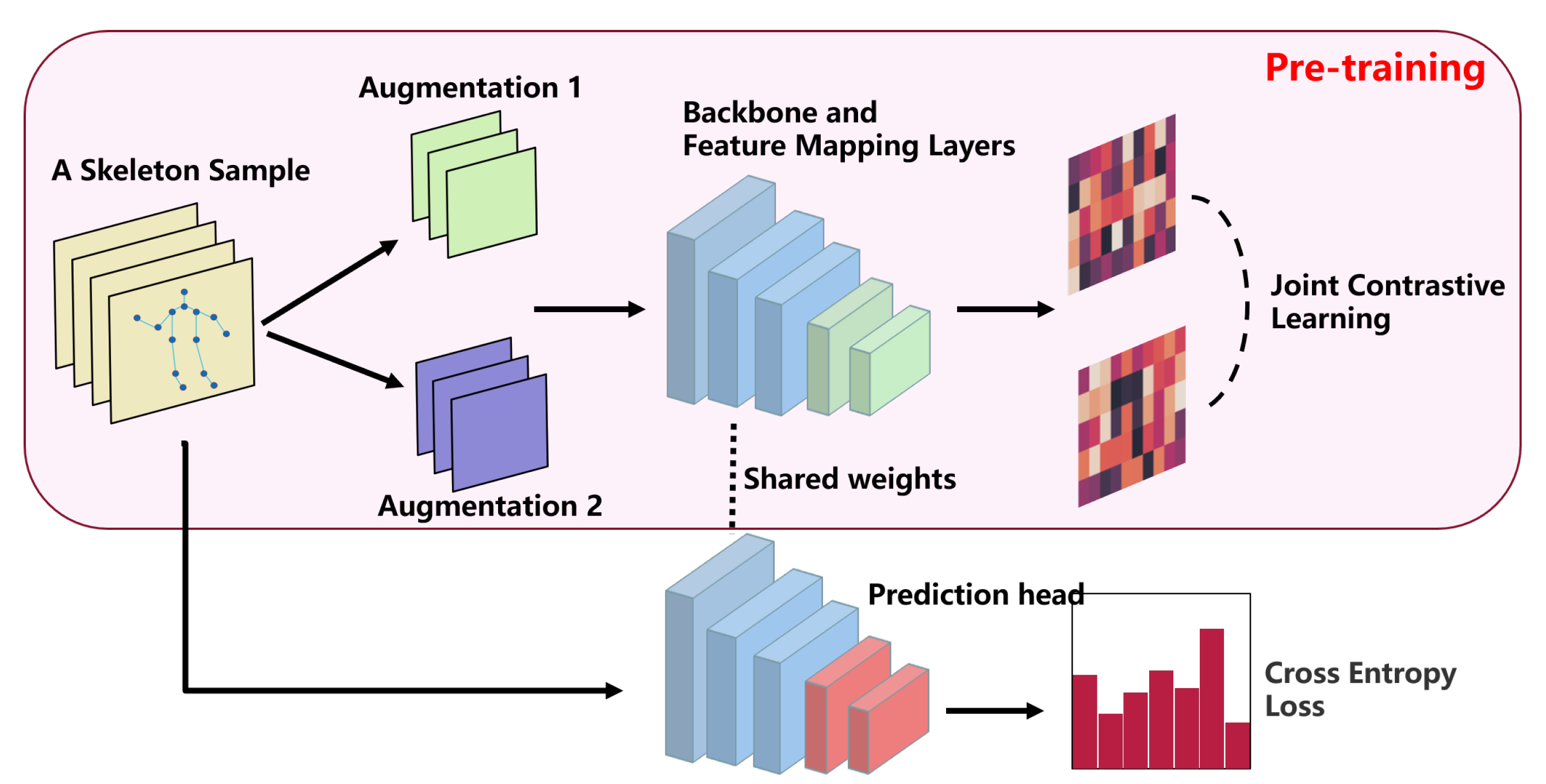
A well-designed pretext task for pre-training aims to learn network weights that are universally applicable and useful to multiple downstream tasks. In terms of architecture, speed of inference is a major consideration in some tasks where the network used is a lightweight network. In contrast, the success of pre-training relies on networks with an excess of parameters. In terms of data, a sufficiently large amount of data is one of the keys to successful pre-training, so a dataset like NTU60 or NTU120 is needed. Finally, in terms of loss design, a contrast loss function needs to be designed according to the pretext task. In Figure 3, we conclude the pre-training framework we explore in this paper, and call the pre-training framework JointContrast. Specifically, given a skeletal sample S , we first generate two new samples S 1 and S 2 aligned in the same world coordinate system by common data augmentation, including random flips, rotations, translations, and scaling. We then feed the samples S 1 and S 2 to the shared backbone network to extract spatio-temporal feature representations F 1 and F 2 . Finally, a contrast loss applied to these two spatio-temporal features is defined: we minimize the feature distance between corresponding joints and maximize the feature distance between non-corresponding joints.
InfoNCE, proposed in [40], is used by most of the unsupervised representational learning methods applied to scene understanding. By treating contrast learning as a dictionary query process, InfoNCE views contrast learning as a classification problem of classifying positive sample pairs into the same class and negative sample pairs into different classes, with a concrete implementation using S o f t M a x loss. Our proposed contrast loss function based on corresponding joints is an improvement on the original InfoNCE.
L = ( i , j ) P l o g e x p ( f 1 I · F 2 j / γ ) ( · , k ) P e x p ( F 1 i · F 2 k / γ )
where P is the set of all positive joint pairs. In this form, we only consider joints that have at least one corresponding joint and do not use additional non-corresponding joints as negative. For a positive joint pair ( i , j ) P , the joint feature F 1 i will be used as the query and F 2 j will be used as the positive key. In addition, we use all joint features F 2 k where ( · , k ) P and k j as the set of negative keys. We summarize the above pre-training process as Algorithm 1.
Algorithm 1 Joint contrast learning algorithm.
  • Require: Backbone NN
  • Require: Skeleton dataset X = { x i }
  • Require: Channels for feature maps D
  • Ensure: Pre-training parameters of the backbone network
  • for Each skeletal sample in the dataset x do
                 Generate two views from x , x 1 and x 2
                 Sampling two transformations T 1 , T 2
                 Compute the features of the skeletal data f 1 , f 2 R N × D by f 1 = N N ( T 1 ( x 1 ) ) and f 2 = N N ( T 2 ( x 2 ) )
                 Compute the loss and update the parameters of the network NN by back propagation using the contrast loss function L ( f 1 , f 2 ) on the corresponding joints
  • end for

3.5. Backbone and Fine-Tuning

In this paper, we use the Graph Convolutional embedding LSTM (GC-LSTM) network as the backbone, which is originally designed in [39] that achieved significant improvement over prior methods. Specifically, we utilize one LSTM layer as joint encoder to model joint representation, and then three GC-LSTM blocks with proposed JAM model discriminative spatialtemporal features. Finally, temporal average pooling is the implementation of average pooling in the temporal domain, and we use the global feature of all joints to predict the class of human action. The graph convolution operation embedded in GC-LSTM enables memory cells to process graph-structured data. By combining our proposed interaction information embedding graph representation, it is capable of representing the joint dependencies between different subjects.
In the previous section we use the correspondence between joints and complete unsupervised pre-training using contrast learning to obtain the pre-trained network parameters. The effects are (1) to make the features corresponding to each joint more dispersed in the feature space and to highlight the unique role played by each joint in the action; (2) to close the feature distance between samples of the same category, making the model more robust. After unsupervised pre-training of the model using data from the source dataset, we initialize the network using the pre-trained parameters and then fine-tune it on the target training set. Unsupervised pre-training work requires a large amount of data, even if that data is unlabeled. We chose NTU120 as the pre-training dataset, which is the largest dataset related to skeletal data with a rich sample of action classes and inter-class diversity.

4. Experiments

4.1. Datasets and Metrics

4.1.1. SBU Dataset

SBU dataset [22] contains the RGB-D sequences of mutual actions, which is constructed by Kinect. There are 282 samples divided into eight categories, which is completed by 7 participants in an experimental environment. Each skeleton sequence contains three-dimensional coordinate information of 15 body joints.

4.1.2. NTU RGB-D Dataset

NTU60 [41] contains a sample of 56,880 actions classified into 60 classes, and the 60 classes are divided into three categories: everyday actions, mutual actions, and health-related actions. Eleven of the classes are interaction actions. All action samples are completed by 40 different experimental participants, which ensures the diversity of each action. Each sample in this dataset is captured simultaneously by three Kinect cameras at different viewing perspectives. In addition to the skeletal data, the dataset also provides RGB video, depth map sequence data. The strengths of this dataset are the richness of the action classes, the sufficiently large number of samples and the diversity of camera views. Recently, the researchers have released an extended version of NTU60, NTU120 [42]. This dataset adds an additional 60 action classes and 57,600 skeletal samples to the original dataset, i.e., NTU120 contains 120 action classes, 26 of which are interactive actions, which makes NTU120 the largest skeletal dataset, and one of the most challenging.

4.1.3. Performance Metrics

The performance of the model is mainly measured using recognition accuracy in the SBU dataset. In NTU60 and NTU120 datasets, there are two ways to evaluate the recognition accuracy: (1) Cross-Subject (CS) accuracy evaluation, the action samples performed by different subjects are divided into the training set and test set; (2) Cross-View (CV) evaluation, the action samples collected by different cameras are divided into the training set and test set.

4.2. Experimental Setup

In each skeleton data, we fix the number of subjects in each scene to 2. For scenes in which only a single person appears, we perform zero padding. For scenes with more than two SUBJECTS, we first calculate the motion distance of all joints of each subject and rank them, and then select the top two subjects with the longest motion distance. Depending on the dataset, we first graphically represent the skeletal data using the proposed IE-Graph to construct joint connection matrices A t and B t to represent the natural connections between joints and our predefined connections between subjects, respectively. To fix the length of the temporal dimension of the skeletal data, we split each skeletal sequence into T subsequences of fixed length and sample a random frame from each subsequence, after sampling, the length of each skeletal sequence is fixed to T. For skeletal samples with original sequence length less than T, we use zero vectors for padding. In addition, we convert the joint coordinates from the camera coordinate system to the human coordinate system according to the parameters inside and outside the camera provided in the dataset, and the purpose of this operation is to eliminate the influence of the camera viewpoint on the data modeling. Specifically, we use the midpoint of the spine as the origin of the human coordinate system, and the new X-axis is the unit vector from the left shoulder to the right shoulder; the new Y-axis is the unit vector from the midpoint of the spine to the vertex of the spine; and the new Z-axis is the direction of increasing depth of field. We use the proposed GC-LSTM which is originally designed in [39] and our JAM to construct the backbone network. We first pre-train this backbone network by the proposed pre-training procedure and contrast loss function to obtain the corresponding parameters. Then the training is performed on the corresponding target training set regarding the action recognition task. In Table 1, we summarily show the hyperparameter settings in this experiment. In addition, the temperature hyperparameter γ for the contrast loss used in pretraining is set to 0.1 . The feature mapping layer is composed of two linear layers, which serve to compare the joint features output from the backbone network. The learnable parameters obtained in the pre-training phase are used to initialize the network in the fine-tuning phase, and the feature mapping layer is discarded in the fine-tuning phase and replaced by a new untrained category prediction head. In the pre-training and training pipeline, we used the AdamW optimizer and set the learning rate to 1 × 10 4 and 1 × 10 3 .

4.3. Results and Discussion

4.3.1. SBU Dataset

Due to the limited data in the SBU dataset, we implemented data augmentation on this dataset where we introduced Gaussian noise in all joint coordinates to enhance the realism of the data and to provide more training samples than the number of the original dataset. In addition, the coordinates of the joints in each skeletal data are performed to be normalized and then fed to the joint feature extraction network. In this dataset, we used three layers of GC-LSTM and a PROPOSED JAM as the backbone network. The feature dimensions of the GC-LSTM are 16, 32, and 32, respectively, and the JAM is set as the last layer of the backbone network. The backbone network is followed by a classification head with full connectivity and an activation function
The results are presented in Table 2. We compare ours with several existing major methods, including LSTM-IRN, VA-LSTM, and GCA-LSTM. Our method achieves similar accuracy as LSTM-IRM. Our method achieves the best performance similar to LSTM-IRM under the accuracy evaluation of SBU dataset. LSTM-IRN introduces Relational Network (RN) in action recognition, which can accomplish feature representation and class prediction by fetching dependencies between joint pairs. Unlike graph convolutional networks, which represent skeletal data as graph structures, this network takes all inter- and intra-target joint pairs as input. the advantage of the representation adopted by LSTM-IRN is that it takes into account the dependencies between all joints. However, such a data representation method introduces redundant information to some extent, because the information complexity of the input features is proportional to the quadratic. Especially in multi-person scenarios, the redundancy of information is further increased. Our proposed method does not introduce redundant information and is equivalent to achieving the same performance as LSTM-IRN based on simplified input features.

4.3.2. NTU60 and NTU120 Datasets

Despite the large number of samples in this dataset, we performed the data augmentation due to the satisfactory performance we achieved with this on the SBU dataset. Reproducing the compared works on our machine, we find that the recognition accuracy of interaction actions is similar to the average accuracy of all actions. This phenomenon indicates that most methods do not fully use the interaction information in the interaction actions.
We report the interaction recognition accuracy on NTU60 and NTU120 in Table 3, where we classify the baseline methods into LSTM-based, CNN-based, GCN-based, and attention-based methods. From the table, we can see that the proposed method achieves the best performance of 94.1 % and 96.8 % under the two evaluation metrics of NTU60, respectively. Most recent work is based on graph convolution or attention network, where they rely not only on manual data representation methods, but also explore implicit dependencies between joints through a data-driven approach. Unlike these approaches, which explore the rich dependency information between joints within a target, we take the understanding of the whole scene and the interaction information between targets as the key information to explore. This is because it is the lack of representation of interaction information that makes it difficult for single-subject action recognition methods to perform well in multi-subjects action settings. However, in addition to predefining some edges in the graph representation, we also share with these methods the learning of dynamic joint dependencies through a data-driven approach. This also brings our approach one step closer and shows better performance. For the 11 interaction action classes in this dataset, our JointContrast respectively achieves 94.1 % and 96.8 % recognition accuracy under Cross-Subject and Cross-View evaluation metrics, which is the best among the baseline methods. In addition to our method itself taking into account the discriminative features required for interaction recognition (including: intra-subject spatial structure information, temporal information, and inter-subjects interaction information), our pre-training with fine-tuning strategy also plays a great help. We will focus on this in our ablation experiments.
As an extended version of the NTU60 dataset, the skeletal data in NTU120 are similar to NTU60 in terms of data form and distribution, but with the increase in the number of classes of actions and samples, the inter-class similarity and intra-class diversity have changed, making the dataset more challenging and posing a greater challenge to the accurate prediction of the models. From the recognition accuracy results presented in Table 3, we can see that the recognition accuracy of all methods decreases under different evaluation metrics, which is in line with expectations. However, again, we can see that the proposed method is the best performing among the compared methods in terms of both Cross-Subject and Cross-View evaluation metrics, achieving 88.2 % and 88.9 % , respectively.
In Figure 4, we show the comparison of the recognition accuracy of our method with ST-TR and MS-G3D methods under the Cross-Subject evaluation accuracy on the NTU60 dataset. We are able to see that the recognition accuracy of our method is better than both ST-TR and MF-F3D in 11 interaction action classes, due to the modeling of spatial, temporal and interaction information and the exploration of the co-occurrence between these features in our method.

4.3.3. Hyper-Parameters Analysis

The performance comparison of hyperparameters K 1 , K 2 is shown in Table 4. K 1 , K 2 do not affect the number of parameters of the model, but have a certain impact on the inference speed of the model. Models (a) and (b) illustrate that performance can be improved by increasing K 2 when K 1 is in a certain region; Comparing models (a) and (c), we improve the performance of the model by increasing the receptive field controlled by K 1 . However, K 1 and K 2 are coupled, and the redundant features increase as K 1 and K 2 increase, which leads to no performance improvement of model (d).

4.4. Ablation Study

4.4.1. Pre-Traning with Contrastive Learning

The finding that pre-training a network on a rich source set can help boost performance once fine-tuned on the target set has been key to the success of many applications. To evaluate the impact of pre-training process on model performance, we select ST-GCN and ST-GCN as the baseline for further ablation study. As shown in Figure 5, for all baselines, the performance of the scratch-trained model lags behind that of pre-trained. From the table, we can see that pre-trained models require more training to achieve optimal performance than models trained from scratch. A recent study suggests the gap between pre-trained and scratch-trained can be closed simply by training more epochs. To this end, We perform additional experiments, training the network with 2× and 3× epochs. We notice that the recognition accuracy does not improve with more extended training, probably because both baselines suffer from over-fitting. The results illustrate the effectiveness of pre-training and the advantages over scratch training.
We pre-train the model with the joint level contrastive loss, bringing corresponding joint features closer and pushing the non-corresponding features farther apart, and Figure 6 shows affinity matrices between joints after pre-training. Most of the previous work uses an attention mechanism to distinguish the specificity of the joint. However, we focus on the uniqueness of the joint and embed it in the features of the joint itself. Joint features more dispersed in the feature space help predict heads to obtain more distinguishable high-order representations for classification.

4.4.2. Interaction Embedding Graph

The proposed IE-Graph models both intra- and inter-subjects relationships within a unified graph structure. To illustrate the broad applicability and validity of proposed IE-Graph, we select two GCN-based methods, GCN-LSTM and ST-GCN, as the baselines which trained from scratch for ablation study. As shown in Table 5, the accuracy of ST-GCN w/ IE-Graph improves by 5.2% compared to one w/o IE-Graph, and GC-LSTM w/ IE-Graph improved by 5.5%. Although the number of corresponding parameters has increased by 10%, we believe the performance improvement is more impressive. This result shows that the proposed IE-Graph adequately extracts the interaction information between subjects and enables the interaction recognition accuracy of the model to be improved. In addition, IE-Graph has wide applicability to most GCN-based methods.
Another interesting phenomenon is that when the baseline uses IG, the recognition accuracy of all actions lags behind mutual actions. We believe that since mutual actions have richer information, the design of IG is more conducive to information embedding. For non-mutual actions, the IG is more like adding a new feature space. Therefore, although the accuracy of all-category action has been improved, the proportion of improvement lags behind mutual action.

4.4.3. Joint Attention

To illustrate the impact of joint attention modules, we compare the performance of models with different numbers of joint attention modules. We fix the position of the joint attention module at the last block of each stage of the model and remove joint attention module from the first to the last stage step-by-step. As shown in Table 6, the baseline GLIA(3A) achieves the highest accuracy. Meanwhile, We found that the joint attention module which is closer to the prediction head is more likely to affect the performance of recognition. Qualitative, the early attention weight will be gradually forgotten by the network, only by constantly reminding the network of the importance of different joints can the network learn a stable attention weights, which is also the reason why GLIA(3A) is the best. Quantitative, We visualize the heatmap of joint attention at different positions as shown in Figure 7. We find that the early attention module is less effective than the deeper ones. From the perspective of the skeleton graph, GCN assigns different weights to edges, and the Joint attention module assigns different weights to vertices, which makes the model stronger and more robust

4.4.4. Bones Information

Numerous experiments show that prior knowledge can improve the performance of the model. For action recognition, bones information is widely used to build 2-stream models. As shown in Table 7, the performance of JointContrast(both) outperforms the joint-stream and bones-stream ones. This phenomenon shows that bones information is beneficial to our JointContrast, because 2-stream contains position information and orientation information. Therefore, our JointContrast is a 2-stream model.

5. Conclusions

Considering the key limitations of the previous works in representation learning and interaction information modeling for interaction recognition, we propose a new representation for skeleton data, named Interactive information Embedding Graph (IE-Graph). With the help of IE-Graph, the model can use graph convolution to represent the intra-subject spatial information and inter-subject interaction information in a uniform manner, which allows us to generalize the single-subject action recognition methods to interaction recognition easily. In addition, we propose a contrastive loss as well as an unsupervised pre-training framework for skeletal-based tasks. Our proposed IE-Graph and pre-training pretext tasks achieve impressive experimental results, but there are still some limitations: (1) compared to data-driven representations, IE-Graph may ignore a few joint dependencies; (2) Limited improvement in model performance from pre-training. Our future works will focus on (1) more flexible and efficient representation of skeleton data and (2) more effective pre-training pretext tasks.

Author Contributions

Conceptualization, J.Z.; methodology, J.Z. and X.J.; software, J.Z. and Z.W.; validation, J.Z., X.J. and Z.W.; formal analysis, Y.L.; investigation, F.C.; resources, G.Y. and L.Z.; data curation, J.Z. and X.J.; writing—original draft preparation, X.J., J.Z. and Z.W.; writing—review and editing, All Authors; visualization, J.Z. and X.J.; supervision, J.Z.; project administration, J.Z.; funding acquisition, J.Z. All authors have read and agreed to the published version of the manuscript.

Funding

This research is partially supported by National Science Foundation of China (No. 62172372, 62272006, 61972438), and Zhejiang Provincial Natural Science Foundation (No. LZ21F030001).

Data Availability Statement

Not applicable.

Conflicts of Interest

The authors declare no conflict of interest.

References

  1. Liu, J.; Shahroudy, A.; Xu, D.; Wang, G. Spatio-temporal lstm with trust gates for 3d human action recognition. In Computer Vision—ECCV 2016; Springer: Berlin/Heidelberg, Germany, 2016; pp. 816–833. [Google Scholar]
  2. Ke, Q.; Bennamoun, M.; An, S.; Sohel, F.; Boussaid, F. A new representation of skeleton sequences for 3d action recognition. In Proceedings of the IEEE Conference on Computer Vision and Pattern Recognition, Honolulu, HI, USA, 21–26 July 2017; pp. 3288–3297. [Google Scholar]
  3. Han, F.; Reily, B.; Hoff, W.; Zhang, H. Space-time representation of people based on 3D skeletal data: A review. Comput. Vis. Image Underst. 2017, 158, 85–105. [Google Scholar] [CrossRef] [Green Version]
  4. Perez, M.; Liu, J.; Kot, A.C. Interaction relational network for mutual action recognition. IEEE Trans. Multimed. 2021, 24, 366–376. [Google Scholar] [CrossRef]
  5. Yang, C.L.; Setyoko, A.; Tampubolon, H.; Hua, K.L. Pairwise adjacency matrix on spatial temporal graph convolution network for skeleton-based two-person interaction recognition. In Proceedings of the 2020 IEEE International Conference on Image Processing (ICIP), Abu Dhabi, United Arab Emirates, 25–28 October 2020; pp. 2166–2170. [Google Scholar]
  6. Nguyen, X.S. Geomnet: A neural network based on riemannian geometries of spd matrix space and cholesky space for 3d skeleton-based interaction recognition. In Proceedings of the IEEE/CVF International Conference on Computer Vision, Montreal, BC, Canada, 11–17 October 2021; pp. 13379–13389. [Google Scholar]
  7. Khaire, P.; Kumar, P. Deep learning and RGB-D based human action, human–human and human–object interaction recognition: A survey. J. Vis. Commun. Image Represent. 2022, 86, 103531. [Google Scholar] [CrossRef]
  8. Gao, F.; Xia, H.; Tang, Z. Attention Interactive Graph Convolutional Network for Skeleton-Based Human Interaction Recognition. In Proceedings of the 2022 IEEE International Conference on Multimedia and Expo (ICME), Taipei, Taiwan, 18–22 July 2022; pp. 1–6. [Google Scholar]
  9. Kasprzak, W.; Piwowarski, P.; Do, V.K. A lightweight approach to two-person interaction classification in sparse image sequences. In Proceedings of the 2022 17th Conference on Computer Science and Intelligence Systems (FedCSIS), Sofia, Bulgaria, 4–7 September 2022; pp. 181–190. [Google Scholar]
  10. Devlin, J.; Chang, M.W.; Lee, K.; Toutanova, K. Bert: Pre-training of deep bidirectional transformers for language understanding. arXiv 2018, arXiv:1810.04805. [Google Scholar]
  11. Radford, A.; Wu, J.; Child, R.; Luan, D.; Amodei, D.; Sutskever, I. Language models are unsupervised multitask learners. OpenAI Blog 2019, 1, 9. [Google Scholar]
  12. Bachman, P.; Hjelm, R.D.; Buchwalter, W. Learning representations by maximizing mutual information across views. Adv. Neural Inf. Process. Syst. 2019, 32, 15535–15545. [Google Scholar]
  13. Tian, Y.; Krishnan, D.; Isola, P. Contrastive multiview coding. In Proceedings of the European Conference on Computer Vision, Glasgow, UK, 23–28 August 2020; pp. 776–794. [Google Scholar]
  14. He, K.; Fan, H.; Wu, Y.; Xie, S.; Girshick, R. Momentum contrast for unsupervised visual representation learning. In Proceedings of the IEEE/CVF Conference on Computer Vision and Pattern Recognition, Seattle, WA, USA, 13–19 June 2020; pp. 9729–9738. [Google Scholar]
  15. Misra, I.; van der Maaten, L. Self-supervised learning of pretext-invariant representations. In Proceedings of the IEEE/CVF Conference on Computer Vision and Pattern Recognition, Seattle, WA, USA, 13–19 June 2020; pp. 6707–6717. [Google Scholar]
  16. Li, B.; Dai, Y.; Cheng, X.; Chen, H.; Lin, Y.; He, M. Skeleton based action recognition using translation-scale invariant image mapping and multi-scale deep CNN. In Proceedings of the 2017 IEEE International Conference on Multimedia & Expo Workshops (ICMEW), Hong Kong, China, 10–14 July 2017; pp. 601–604. [Google Scholar]
  17. Yan, S.; Xiong, Y.; Lin, D. Spatial temporal graph convolutional networks for skeleton-based action recognition. In Proceedings of the Thirty-Second AAAI Conference on Artificial Intelligence, New Orleans, LA, USA, 2–7 February 2018. [Google Scholar]
  18. Li, M.; Chen, S.; Chen, X.; Zhang, Y.; Wang, Y.; Tian, Q. Actional-structural graph convolutional networks for skeleton-based action recognition. In Proceedings of the IEEE/CVF Conference on Computer Vision and Pattern Recognition, Long Beach, CA, USA, 15–20 June 2019; pp. 3595–3603. [Google Scholar]
  19. Shi, L.; Zhang, Y.; Cheng, J.; Lu, H. Decoupled spatial-temporal attention network for skeleton-based action-gesture recognition. In Proceedings of the Asian Conference on Computer Vision, Kyoto, Japan, 30 November 30–4 December 2020. [Google Scholar]
  20. Liu, Y.; Zhang, H.; Xu, D.; He, K. Graph transformer network with temporal kernel attention for skeleton-based action recognition. Knowl.-Based Syst. 2022, 240, 108146. [Google Scholar] [CrossRef]
  21. Ji, Y.; Cheng, H.; Zheng, Y.; Li, H. Learning contrastive feature distribution model for interaction recognition. J. Vis. Commun. Image Represent. 2015, 33, 340–349. [Google Scholar] [CrossRef]
  22. Yun, K.; Honorio, J.; Chattopadhyay, D.; Berg, T.L.; Samaras, D. Two-person interaction detection using body-pose features and multiple instance learning. In Proceedings of the 2012 IEEE Computer Society Conference on Computer Vision and Pattern Recognition Workshops, Providence, RI, USA, 16–21 June 2012; pp. 28–35. [Google Scholar]
  23. Ouyed, O.; Allili, M.S. Group-of-features relevance in multinomial kernel logistic regression and application to human interaction recognition. Expert Syst. Appl. 2020, 148, 113247. [Google Scholar] [CrossRef]
  24. Ji, Y.; Ye, G.; Cheng, H. Interactive body part contrast mining for human interaction recognition. In Proceedings of the 2014 IEEE International Conference on Multimedia and Expo Workshops (ICMEW), Chengdu, China, 14–18 July 2014; pp. 1–6. [Google Scholar]
  25. Liu, B.; Ju, Z.; Liu, H. A structured multi-feature representation for recognizing human action and interaction. Neurocomputing 2018, 318, 287–296. [Google Scholar] [CrossRef] [Green Version]
  26. Li, M.; Leung, H. Multiview skeletal interaction recognition using active joint interaction graph. IEEE Trans. Multimed. 2016, 18, 2293–2302. [Google Scholar] [CrossRef]
  27. Ito, Y.; Morita, K.; Kong, Q.; Yoshinaga, T. Multi-Stream Adaptive Graph Convolutional Network Using Inter-and Intra-Body Graphs for Two-Person Interaction Recognition. IEEE Access 2021, 9, 110670–110682. [Google Scholar] [CrossRef]
  28. Pang, Y.; Ke, Q.; Rahmani, H.; Bailey, J.; Liu, J. IGFormer: Interaction Graph Transformer for Skeleton-based Human Interaction Recognition. In Proceedings of the European Conference on Computer Vision, Tel Aviv, Israel, 23–27 October 2022; pp. 605–622. [Google Scholar]
  29. Jia, X.; Zhang, J.; Wang, Z.; Luo, Y.; Chen, F.; Xiao, J. JointContrast: Skeleton-Based Mutual Action Recognition with Contrastive Learning. In Proceedings of the PRICAI 2022: Trends in Artificial Intelligence: 19th Pacific Rim International Conference on Artificial Intelligence, PRICAI 2022, Shanghai, China, 10–13 November 2022; Part III. pp. 478–489. [Google Scholar]
  30. Chiu, S.Y.; Wu, K.R.; Tseng, Y.C. Two-Person Mutual Action Recognition Using Joint Dynamics and Coordinate Transformation. In Proceedings of the CAIP 2021: The 1st International Conference on AI for People: Towards Sustainable AI, CAIP 2021, Bologna, Italy, 20–24 November 2021; p. 56. [Google Scholar]
  31. Yang, H.; Yan, D.; Zhang, L.; Sun, Y.; Li, D.; Maybank, S.J. Feedback graph convolutional network for skeleton-based action recognition. IEEE Trans. Image Process. 2021, 31, 164–175. [Google Scholar] [CrossRef] [PubMed]
  32. Chen, T.; Kornblith, S.; Norouzi, M.; Hinton, G. A simple framework for contrastive learning of visual representations. In Proceedings of the International Conference on Machine Learning, PMLR, Virtual Event, 13–18 July 2020; pp. 1597–1607. [Google Scholar]
  33. Chen, T.; Kornblith, S.; Swersky, K.; Norouzi, M.; Hinton, G.E. Big self-supervised models are strong semi-supervised learners. Adv. Neural Inf. Process. Syst. 2020, 33, 22243–22255. [Google Scholar]
  34. Singh, A.; Chakraborty, O.; Varshney, A.; Panda, R.; Feris, R.; Saenko, K.; Das, A. Semi-supervised action recognition with temporal contrastive learning. In Proceedings of the IEEE/CVF Conference on Computer Vision and Pattern Recognition, Nashville, TN, USA, 20–25 June 2021; pp. 10389–10399. [Google Scholar]
  35. Radford, A.; Kim, J.W.; Hallacy, C.; Ramesh, A.; Goh, G.; Agarwal, S.; Sastry, G.; Askell, A.; Mishkin, P.; Clark, J.; et al. Learning transferable visual models from natural language supervision. In Proceedings of the International Conference on Machine Learning, PMLR, Online, 6–14 December 2021; pp. 8748–8763. [Google Scholar]
  36. Qian, R.; Meng, T.; Gong, B.; Yang, M.H.; Wang, H.; Belongie, S.; Cui, Y. Spatiotemporal contrastive video representation learning. In Proceedings of the IEEE/CVF Conference on Computer Vision and Pattern Recognition, Nashville, TN, USA, 20–25 June 2021; pp. 6964–6974. [Google Scholar]
  37. Zamini, M.; Reza, H.; Rabiei, M. A Review of Knowledge Graph Completion. Information 2022, 13, 396. [Google Scholar] [CrossRef]
  38. Guo, L.; Wang, W.; Sun, Z.; Liu, C.; Hu, W. Decentralized knowledge graph representation learning. arXiv 2020, arXiv:2010.08114. [Google Scholar]
  39. Si, C.; Chen, W.; Wang, W.; Wang, L.; Tan, T. An attention enhanced graph convolutional lstm network for skeleton-based action recognition. In Proceedings of the IEEE/CVF Conference on Computer Vision and Pattern Recognition, Long Beach, CA, USA, 15–20 June 2019; pp. 1227–1236. [Google Scholar]
  40. Oord, A.v.d.; Li, Y.; Vinyals, O. Representation learning with contrastive predictive coding. arXiv 2018, arXiv:1807.03748. [Google Scholar]
  41. Shahroudy, A.; Liu, J.; Ng, T.T.; Wang, G. Ntu rgb+ d: A large scale dataset for 3d human activity analysis. In Proceedings of the IEEE Conference on Computer Vision and Pattern Recognition, Las Vegas, NV, USA, 27–30 June 2016; pp. 1010–1019. [Google Scholar]
  42. Liu, J.; Shahroudy, A.; Perez, M.; Wang, G.; Duan, L.Y.; Kot, A.C. Ntu rgb+ d 120: A large-scale benchmark for 3d human activity understanding. IEEE Trans. Pattern Anal. Mach. Intell. 2019, 42, 2684–2701. [Google Scholar] [CrossRef] [Green Version]
  43. Zhu, W.; Lan, C.; Xing, J.; Zeng, W.; Li, Y.; Shen, L.; Xie, X. Co-occurrence feature learning for skeleton based action recognition using regularized deep LSTM networks. In Proceedings of the AAAI Conference on Artificial Intelligence, Phoenix, AZ, USA, 12–17 February 2016; Volume 30. [Google Scholar]
  44. Zhang, P.; Lan, C.; Xing, J.; Zeng, W.; Xue, J.; Zheng, N. View adaptive recurrent neural networks for high performance human action recognition from skeleton data. In Proceedings of the IEEE International Conference on Computer Vision, Venice, Italy, 22–29 October 2017; pp. 2117–2126. [Google Scholar]
  45. Liu, J.; Wang, G.; Duan, L.Y.; Abdiyeva, K.; Kot, A.C. Skeleton-based human action recognition with global context-aware attention LSTM networks. IEEE Trans. Image Process. 2017, 27, 1586–1599. [Google Scholar] [CrossRef] [PubMed] [Green Version]
  46. Wu, F.; Souza, A.; Zhang, T.; Fifty, C.; Yu, T.; Weinberger, K. Simplifying graph convolutional networks. In Proceedings of the International Conference on Machine Learning, PMLR, Long Beach, CA, USA, 9–15 June 2019; pp. 6861–6871. [Google Scholar]
  47. Cho, S.; Maqbool, M.; Liu, F.; Foroosh, H. Self-attention network for skeleton-based human action recognition. In Proceedings of the IEEE/CVF Winter Conference on Applications of Computer Vision, Seattle, WA, USA, 13–19 June 2020; pp. 635–644. [Google Scholar]
  48. Zhang, P.; Lan, C.; Xing, J.; Zeng, W.; Xue, J.; Zheng, N. View adaptive neural networks for high performance skeleton-based human action recognition. IEEE Trans. Pattern Anal. Mach. Intell. 2019, 41, 1963–1978. [Google Scholar] [CrossRef] [PubMed] [Green Version]
  49. Plizzari, C.; Cannici, M.; Matteucci, M. Spatial temporal transformer network for skeleton-based action recognition. In Proceedings of the International Conference on Pattern Recognition, Milan, Italy, 10–15 January 2021; pp. 694–701. [Google Scholar]
  50. Cheng, K.; Zhang, Y.; He, X.; Chen, W.; Cheng, J.; Lu, H. Skeleton-based action recognition with shift graph convolutional network. In Proceedings of the IEEE/CVF Conference on Computer Vision and Pattern Recognition, Seattle, WA, USA, 13–19 June 2020; pp. 183–192. [Google Scholar]
  51. Liu, Z.; Zhang, H.; Chen, Z.; Wang, Z.; Ouyang, W. Disentangling and unifying graph convolutions for skeleton-based action recognition. In Proceedings of the IEEE/CVF Conference on Computer Vision and Pattern Recognition, Seattle, WA, USA, 13–19 June 2020; pp. 143–152. [Google Scholar]
Figure 1. IE-Graph Representation: The joint edge (black) links the joints within the same subject, and the subject edge (red) links the joints of the same kind between different subjects, which models the interactive information. For brevity, we show only a portion of the subject edges in the figure.
Algorithms 16 00190 g001
Figure 2. The Joint Attention Module first pools the spatial-temporal feature map, and then uses the linear layer and Softmax to obtain the attention weight, which is used to perform element multiplication with the original feature map. Finally, each joint receives different attention in the feature map.
Algorithms 16 00190 g002
Figure 3. Our framework consists of two parts: pre-training and fine-tuning. In pre-training, two training samples are generated from each raw data by common data augmentation. With the help of IE-Graph, we feed the samples to the network to extract joint features and update the parameters using the proposed contrastive loss. In fine-tuning, the pre-trained weights are used as the initialization and are further refined on the target downstream task. In addition, we add a prediction head to complete the recognition.
Algorithms 16 00190 g003
Figure 4. The interaction recognition accuracy on the NTU60 dataset: ST-TR, MS-G3D and our JointContrast.
Algorithms 16 00190 g004
Figure 5. Comparison in terms of interaction recognition accuracy of models w/ and w/o pre-training on the NTU60 dataset. schedules means the training epochs.
Algorithms 16 00190 g005
Figure 6. The affinity matrices between joints after pre-training, where the numbers represent the different joints.
Algorithms 16 00190 g006
Figure 7. Attention visualization for the handshake action, where the top ones corresponds to the shallow layer of the network. The attention weights are normalized.
Algorithms 16 00190 g007
Table 1. The hyperparameter settings in this experiment.
DatasetTMN K 1 K 2
SBU4021521
NTU60 & NTU12030022521
Table 2. The interaction recognition accuracy on the SBU dataset, accmeans recognition accuracy.
Methodsacc
CFDM [21]89.4%
ST-LSTM [1]93.3%
Co-occurrence LSTM [43]90.4%
VA-LSTM [44]97.2%
2sGCA-LSTM [45]94.9%
SGCConv [46]94.0%
LSTM-IRN [4]98.2%
JointContrast (ours)98.2%
Table 3. The interaction recognition accuracy under Cross-Subject (CS) and Cross-View (CV) accuracy evaluation on NTU60 and NTU120.
NTU60NTU120
MethodsCS acc (%)CV acc (%)CS acc (%)CV acc (%)
ST-LSTM [1]83.087.363.066.6
LSTM-IRN [4]90.593.577.779.6
AGC-LSTM [39]89.295.073.073.3
SAN [47]88.293.5--
VACNN [48]88.994.7--
ST-GCN [17]83.388.7--
AS-GCN [18]87.695.282.983.7
ST-TR [49]90.896.585.787.1
2sshift-GCN [50]90.396.086.186.7
MS-G3D [51]91.796.1--
2sKA-AGTN [20]90.496.186.788.2
JointContrast (ours)94.196.888.288.9
Table 4. Comparison in terms of interaction recognition accuracy of K 1 , K 2 .
MethodsK1K2CS acc (%)
(a)2193.3
(a)2293.8
(b)3194.1
(c)3294.1
Table 5. Comparison in terms of interaction recognition accuracy of the models w/ and w/o IE-Graph on the NTU60 dataset.
MethodsCS acc (%)CV acc (%)IE-GraphParameters ( 10 7 )
ST-GCN83.388.7w/o1.2
ST-GCN88.592.1w/1.3
GC-LSTM89.295.0w/o1.17
GC-LSTM93.796.1w/1.28
Table 6. Comparison in terms of interaaction recognition accuracy of Joint Attention Module.
MethodsCS acc (%)Decrease (%)
GLIA(3-A)93.7-
GLIA(2-A)93.10.6
GLIA(1-A)91.71.4
GLI(non-A)89.02.7
Table 7. Comparison in terms of interaction recognition accuracy of joint-, bone- and both-stream.
MethodsJointBoneCS acc (%)
JointContrast (joints)yes-93.3
JointContrast (bones)-yes92.8
JointContrast (both)yesyes94.7
Disclaimer/Publisher’s Note: The statements, opinions and data contained in all publications are solely those of the individual author(s) and contributor(s) and not of MDPI and/or the editor(s). MDPI and/or the editor(s) disclaim responsibility for any injury to people or property resulting from any ideas, methods, instructions or products referred to in the content.

