
Pushing the Limits of Clingo’s Incremental Grounding and Solving Capabilities in Practical Applications
1
Elemental Cognition, Inc., New York, NY 10169, USA
2
Department of Decision & System Sciences, Erivan K. Haub School of Business, Saint Joseph’s University, Philadelphia, PA 19131, USA
*
Author to whom correspondence should be addressed.
Algorithms 2023, 16(3), 169; https://doi.org/10.3390/a16030169
Submission received: 16 February 2023
/
Revised: 15 March 2023
/
Accepted: 18 March 2023
/
Published: 20 March 2023
(This article belongs to the Special Issue Hybrid Answer Set Programming Systems and Applications)
Abstract
:Incremental techniques aim at making it possible to improve the performance of the grounding and solving processes by reusing the results of previous executions. Clingo supports both incremental grounding and incremental solving computations. In order to leverage incremental computations in clingo, the incremental fragments of ASP programs must satisfy certain safety-related conditions. In a number of problem domains and reasoning tasks, these conditions can be satisfied in a fairly straightforward way. However, we have observed that in certain practical applications, satisfying the conditions becomes more challenging, to the point that it is sometimes unclear how or even if it is possible to leverage incremental computations. In this paper, we report our findings, and ultimate success, with the use of incremental grounding and solving techniques in one of these challenging cases. We describe the domain, which is linked to a large practical application, discuss the challenges we faced in attempting to leverage incremental computations, and then describe the techniques that we developed, in particular at the level of methods for encoding the domain knowledge and of algorithms supporting the intended interleaving of grounding and solving. We believe that our findings may provide valuable information to practitioners facing similar challenges and ultimately increase the adoption of clingo’s incremental capabilities for complex practical applications.
1. Introduction
Answer Set Programming (ASP) [1,2] provides a convenient paradigm for tackling complex modeling and reasoning tasks. In many cases, the performance of ASP-based solutions is also sufficient for practical applications, as demonstrated by a healthy stream of publications (see, e.g., [3]).
Since the first demonstration of the viability of ASP for practical, industry-sized applications [4], the community has experienced a constant alternation between more challenging application domains, more sophisticated modeling constructs, and correspondingly more powerful solving technologies.
Typically, the computation of the answer sets of ASP programs is performed in two steps, the grounding step and the solving step, discussed later. In recent years, the clingo solver [5] introduced support for incremental (or “multi-shot”) computations in both grounding and solving [6,7,8]. As long as the conditions of the Module Theorem are satisfied [9,10], the computation of answer sets of an ASP program can be performed incrementally. This often leads to substantial performance improvements, since one can leverage and build upon the results of previous, computationally smaller, runs.
In our use of ASP for practical applications, we recently found ourselves faced with the task of computing the evolution of the state of a dynamic domain [11,12], and while the use of ASP for such a task is not new, our situation was complicated by a number of factors. At its core, our application [13,14] formalized and reasoned about policies [15] aimed at determining an individual’s readiness to perform activities (work, school, sports, etc.) during the peak of the COVID-19 pandemic. At that time, the task of easing COVID-19 lockdown restrictions was complicated due to a variety of factors, including the uncertainty about the way in which the virus spread and the challenges in adapting pre-existing environments that were not meant to limit the spread of such an aggressive airborne virus. A practice commonly used with the aim of reducing risks consisted in adopting policies that determined an individual’s fitness to access an environment or perform an activity. For instance, for an employee to be granted access an office environment on a given day, the person may be required to have been symptom-free for the past 24 h and not have been in contact with sick individuals for the past 7 days. A student returning to campus from another state may be required to have tested negative for COVID-19 in the past 5 days or he/she would have to quarantine for 14 days; then again, in some policies it was possible to shorten such quarantines under certain very specific conditions (e.g., a particular battery of tests providing the necessary results), but it was also possible that the quarantine would need to be extended if other conditions became true (e.g., having certain symptoms). Policies often became very complex to both describe and understand. Due to how rapidly conditions and recommendations were changing, and to the many ramifications of resuming regular activities or not, it was paramount to have tools that simplified the task of developing and enforcing policies. Particularly, it was essential to enable (1) the rapid development of policies, (2) trust that the implementation of the policies reflected the original intent, and (3) transparency of the decisions made by such implementations. From the perspective of an application aimed at serving as a decision-support system for sizable communities such as universities or large companies, each with its own policies:
- Modeling the policies involved capturing potentially complex interactions among time-delayed ramifications of observations;
- Histories of observations may have to be considered for each individual;
- The application needed to address a continuous stream of observations about both current moments as well as past time periods, due to testing and communication backlogs;
- Past observations may cause the withdrawal of previously held expectations, and thus have to be addressed non-monotonically;
- Because the system was intended to be accessed not only by administrators through their workstations but also by community members directly on their smartphones, the system had to be capable of producing a snapshot of a user’s readiness state weeks into the future in real time;
- Finally, the system was ultimately intended to be hosted on a large cloud infrastructure where computation may need to be moved from one node to another on very short notice. As a result, it had to be possible to conduct all computations in a stateful manner, so that the state of the computation could be saved and reloaded when execution was moved from a node to another.
Consequently, there were a number of important requirements imposed on the reasoning component: the component had to be able to generate and reason about trajectories often exceeding 100 discrete time steps and expected to be 3–5 times longer after deployment; the domain involved the need to represent wall-clock time and durative aspects, either in the form of actions with duration or of (default) fluents with duration; the reasoning component had to be capable of producing a full trajectory in no more than 5 s on average.
Preliminary experiments showed that single-shot computation with clingo was problematic, since the execution times for representative examples were frequently well over 5 s and in approximately 20–25% of cases were above the timeout threshold of 1 h. While the use of incremental computations to speed up the computation was attractive, it was made complicated by the fact that straightforward encodings led to the violation of the conditions of the Module Theorem, making it impossible to apply the current incremental technologies.
In this paper, we report on an approach whose development was prompted by the application described above. The approach leverages incremental techniques for the computation of long (100 or more discrete time steps) trajectories of a dynamic domain in the presence of durative actions or fluents. The approach leverages an incremental, fix-point computation, which not only ensures the satisfaction of the conditions of the Module Theorem and the applicability of clingo’s incremental API, but also yields substantial performance improvements over the non-incremental alternatives. In our experiments, the computations never timed out and the average time was well within the 5 s threshold even on household hardware. This confirms the exceptional capabilities of clingo’s support for incremental computations and demonstrates that certain restrictions on the use of such features can be overcome with suitable representation techniques and algorithms.
Specifically, the contributions of this paper are: (a) an approach for representing knowledge about the durative aspects of dynamic domains that is suitable for processing with incremental techniques; (b) a set of algorithms that leverage clingo’s incremental computation capabilities while avoiding problems related to the conditions of the Module Theorem and substantially improve performance compared to non-incremental approaches; (c) another set of algorithms that build upon the core ones to provide features useful for use in user-facing applications and in cloud-based execution platforms.
The paper is organized as follows. We begin by providing an introduction on necessary background concepts. That is followed by Section 3, where we describe our approach to representing knowledge in a way that is suitable for incremental computations. In the following two sections, we discuss the algorithms we developed for leveraging clingo’s support for incremental computations. In Section 6, we report on our experimental evaluation of the approach. Section 7 and Section 8 discuss extensions of the approach that are geared toward practical use in user-facing applications. We close the paper by summarizing our work and drawing conclusions.
2. Preliminaries
ASP is a declarative programming paradigm based on logic programming under the answer set semantics. An ASP program is a set of rules of the following form:
where c, ’s, and ’s are first-order literals and do represent (default) negation.Intuitively, a rule states that if s are believed to be true and none of the s are believed to be true, then c must be true. c is called the head of the rule and is its body. Additionally, given a rule r, and , respectively, called the positive and negative body, denote the sets and . If the body of a rule is absent, the rule is called fact, its head is always true, and the ← symbol is omitted. If the head of a rule is absent, then the rule is called constraint (or denial), and its body is never allowed to be satisfied.
A rule that contains first-order variables is called non-ground and it is considered to be a shortcut for the set of its ground instances, i.e., the ground rules that can be obtained by replacing the variables by all possible ground terms of the language. The semantics of ASP programs, discussed next, is thus given in terms of ground programs, i.e., sets of ground rules.
Let be a ground program. An interpretation I of is a set of ground literals occurring in . The body of a rule r is satisfied by I if and . A rule r is satisfied by I if the body of r is satisfied by I implies . When c is absent, r is a constraint and is satisfied by I if its body is not satisfied by I. I is a model of if it satisfies all rules in .
For an interpretation I and a program , the reduct of with regard to I (denoted by ) is the program obtained from by deleting (i) each rule r such that , and (ii) all expressions of the form in the bodies of the remaining rules. Given an interpretation I, observe that the program is a program with no occurrence of . An interpretation I is an answer set of if I is the least model (with regard to ⊆) of .
Several extensions have been introduced to simplify the use of ASP. In this paper, we make use of a restricted form of the aggregate of clingo, where an expression is true if v is equal to the minimum (numerical) value of X such that are true. We also use the shorthand to denote the set of rules and .
While for our application we rely on action languages [11] for a compact and high-level representation of policies, for simplicity of presentation in this paper we represent the behavior of the domain directly using ASP rules. We follow the typical approach for such a representation—see, e.g., [4]. Let be a set of actions and be a set of fluents, where a fluent is a (Boolean) property of the domain whose truth value may change over time. Let be a set of integers intuitively corresponding to discrete time steps in the evolution of the state of the domain. A fluent literal is a fluent f or its (classical) negation . A state is a complete and consistent set of fluent literals from . (Without loss of generality, for sake of simplicity we adopt a simpler definition than that of [2]). A literal of the form (resp., ) indicates that fluent f is true (or false) at time step t. A literal indicates that action a occurs at time step t. A literal indicates that t belongs to . A literal states that are immediately consecutive steps from , in the sense that there is no other time step such that . The set of laws (often called action description) that affect the evolution of the state of the domain is represented by means of ASP rules. For example, a dynamic causal law stating that pushing a button b of a given light bulb l to light up may be captured by a rule:
A state constraint stating that, when the light bulb is on, it is also hot, may be captured by a rule:
The description of the behavior of the system (at least in simple cases) is completed by the inertia axioms [16,17], which intuitively state that things tend to stay as they are. They can be compactly represented in ASP with rules such as
A thorough discussion on dynamic domains and on their representation in ASP is beyond the scope of this paper. We refer the interested reader to [11] for details.
Next, we provide a basic introduction on the support for incremental computations in clingo. Due to the complexity of the topic, we limit the scope of the discussion to only what is strictly necessary for the description of our approach, and refer the interested reader to [6,7] for a thorough discussion. Additionally, we focus our discussion to the incremental computation facilities provided by clingo 5.4.0, the version of the solver available at the time of the development of our approach.
Incremental ASP programs. For incremental computations, an ASP program is conceptually partitioned into one or more modules. Each module is identified by a directive of the form:
where is a unique identifier for the module (in practice, clingo allows for repeated directives, but all rules labeled by such directives are internally combined into the same, unique module) and is a potentially empty list of constant symbols acting as parameters of the module. Such parameters are allowed to occur in the rules of the module in any place that is syntactically valid for a constant symbol. The only module that clingo processes by default is the module, which takes no parameters. All other modules can be dynamically added to the computation by the programmer. When that happens, the programmer will also specify the values of the module’s parameters, if any. If the module has parameters, then what is added to the computation is the instance of the module with regard to the parameter values provided, where instance in this case refers to the set of rules obtained by replacing, in all rules of the module, all parameters’ constant symbols by their corresponding values.
Clingo allows a programmer to label certain literals as external. Such a label indicates to clingo that the truth value of those literals may be determined by rules added to the program at a later time, or even by direct truth assignment by the programmer via the and API functions. In terms of internal handling of rules, clingo treats external literals as module inputs, which prevents those literals and the rules that contain them from being simplified away when their truth value is undefined. External literals are declared by directives of the form:
where , and ’s are sequences of ASP variables, is the (non-ground) literal being declared external, and are a potentially empty set of conditions refining of which the subset of the ground instances of is to be declared external. For practical purposes, one can view the role of the elements of the directive to be similar to those of a rule of the form , although of course an directive has no bearing on the truth value of . External declarations are convenient, in combination with and , for enabling and disabling parts of a module, or of a module as a whole, because they act together in dynamically asserting that a literal, which may be in the body of a rule, is true or false. The recommended practice [7] for designing a set of rules that can be removed from a program being processed in an incremental fashion is to introduce suitable external literals in their bodies. When the external literals are set to true (via ), the rules are enabled and used by the solver. When the rules are to be removed from the program, the external literals that control their application are set to false and released by means of . When that happens, one should also call clingo function , which adjusts the internal state of grounder and solver after information has been retracted.
Incremental computations in clingo. As we mentioned earlier, clingo supports both incremental grounding and incremental solving. Incremental grounding refers to the ability to ground modules in separate stages. When a module is grounded (or an instance of a module, when the module has parameters), it is added to the set of ground rules that clingo maintains. Incremental solving refers to clingo’s ability to store and update the state of the search process across multiple solving calls. When a new call is performed by a programmer, clingo uses the current state of the search process as the starting point of the computation. This approach can potentially yield substantial time savings. As a (trivial) example, consider the case in which one has already grounded and solved a large ASP program and is now interested in adding a new rule. As long as the rule satisfies certain properties, clingo can simply update the truth values of the literals affected by the new rule and avoid repeating the computations linked with the initial program. To make this possible, clingo allows for incremental grounding and solving steps to be interleaved, making it possible for one to ground and solve part of a program, then ground an additional module with respect to the set of ground literals determined by the previous grounding and solving run. As a result, the grounding of the new module may be substantially smaller and cheaper to compute than if the initial program and the new module had been grounded in a single operation.
The Module Theorem. The conditions under which modules can incrementally added to an existing program are given by the Module Theorem [9,10]. We provide here a summary of this topic adapted from [7]. A module is a triple consisting of a ground logic program P along with sets I and O of ground input and output literals such that:
- ,
- , and
where is the set of heads from all rules of P and . A set X of ground literals is an answer set of a module if X is an answer set of . Two modules and are compositional if
- , and
- or for every strongly connected component C of .
The join of and is the module defined as:
According to the Module Theorem, if and are compositional, then (a) their join is defined and (b) its answer sets can be obtained from the answer sets of and as follows:
A set X of ground literals is an answer set of iff for answer sets and of and respectively, such that .
Two very important ramifications of the definition of compositionality and of its role in the Module Theorem are that (i) all rules defining a (ground) literal must belong to the same module, and that (ii) all positive rule cycles must remain confined within individual modules. These requirements impose significant restrictions on the applicability of incremental computations in clingo. Consider for instance the following program:
Furthermore, consider the sequence of clingo calls , which intuitively grounds and solves the module, and then attempts to ground module . The second call to the function will trigger an error, because s is defined in multiple modules.
3. Domain Representation
As we mentioned earlier, durative elements are an important component of the kinds of dynamic domains our application was tasked to tackle. For example, according to certain policies, an individual that had come in contact with sick individuals was not allowed to return to work for 7 days from the contact. If they happened to come in contact again with sick individuals during that period, the period would be extended correspondingly. Information received on positive and negative tests, as well as the types of tests, would also impact one’s readiness to return to their regular activities.
Another important aspect of the domains we considered is the fact that a number of their properties appear to lend themselves to be naturally represented as default fluents, i.e., fluents whose truth value will default to a set one unless actively changed by other laws. Assuming that inertial and default fluents are partitioned by a suitable type relation, e.g., , the inertia axioms shown in Section 2 can be easily restricted to inertial fluents by adding a condition , and the behavior of default fluents can be captured by a rule such as
Some researchers further distinguish between positively defined default fluents and negatively defined default fluents depending on their default truth value, and while in practice we did make this distinction, we disregard this detail for the sake of simplicity of presentation, and only consider default fluents whose truth value defaults to false.
We should mention here that in the rest of this paper we make the assumption that action descriptions are deterministic, i.e., they yield no more than one trajectory from any initial state considered (see, e.g., [18] for a discussion on syntactic conditions that ensure determinism of action descriptions), and are strongly consistent, in the sense that they yield at least one trajectory from any initial state considered.
In the context of the domains we tackled, default durative fluents play a critical rule. For instance, in the example above, by default one was allowed to go to work, but was disallowed to do so for 7 days from an exposure (or, to be precise, from the latest exposure). While some of the aspects of durative fluents can be captured by means of actions with duration, in our application domain durative fluents provide a more natural representation. As it will become clear later, the results discussed in this paper apply both to durative fluents and to actions with duration. Thus, without loss of generality, we focus our discussion on durative fluents.
The representation of the duration of these fluents also requires the ability to reason about “wall-clock” time. Mechanisms for handling “wall-clock” time in the context of action languages and ASP-based domain representations have been explored with a certain degree of success, see, e.g., [19]. These approaches make it possible to model complex continuous and non-linear dynamics by leveraging Constraint ASP (CASP) [20], which combines ASP solving with numerical constraint solving. On the other hand, our preliminary evaluation showed that they also introduce a fair amount of complexity in the representation and do not appear to solve the performance problems inherent in the handling of trajectories with 100 or more discrete time steps. We also considered additive fluents [21] for the representation, but once again they seemed to tackle a somewhat different problem from ours and did not seem to solve the performance challenges we were facing.
As a result, we opted for a more direct representation of (default) durative fluents and of “wall-clock” time. In our approach, the numerical value of time steps is associated with the corresponding “wall-clock” time from a given reference time, while the time resolution of such time steps is application-dependent. In our case, time steps were associated with the time elapsed in seconds from the reference time. The amount of time left before a fluent f returns to its default value is formalized by a literal , intuitively expressing that there are l time units left (or seconds in our case), at time t, before f returns to its default (negative) value. Suitable defaults make it possible to calculate the amount of time left at any time step of interest. Simple extensions of the laws we discussed in Section 2 reset the amount of time left when necessary, e.g., if an observation is received that the subject was exposed to a sick individual and, as a result, the isolation is extended.
This approach makes it necessary for the extension of relation to be determined by the rules of the program, and based on observed needs. Note that this is different from typical approaches for reasoning about dynamic domains in ASP, where one relies on the relation to be defined as part of the input. Consider a case in which a certain set of conditions that are true at time t causes default fluent f to become true and remain true for duration d. In our approach, this is captured by the following set of rules:
The first two rules modify the truth value of the fluent and set the amount of time left before the fluent reverts to its default value. The third rule is responsible for extending the timeline: it states that a time step should be added to the timeline if not already present. (The role of the first argument will become clear later). The timeline is extended in order to allow for the reasoning component to reason about the point at which the default will revert to its default value (that is, unless of course other causes intervene to prevent that).
The formalization of the behavior of durative fluents is thus given by (9) together with:
The first four rules of (11) ensure that the amount of time left is correctly updated from one time step to the next. The last rule captures the inertial behavior of default fluents while they are set to true for a certain amount of time.
Due to our use of a sparse representation of the timeline, we also need to refine the definition of relation , which is accomplished by the rule:
Note the use of clingo’s aggregate to identify the time step that immediately follows T.
The ASP-based reasoning component of our application is designed to take in input a set of observations about the truth value of fluents. In practice, the observations encode the results and types of tests, information about close contacts and travel, self-reported or observed symptoms, etc. Following the approaches from the related literature (e.g., [22]), we represent observations by means of statements of the form
where l is a fluent literal and t is a time step. Intuitively, the statement says that the fluent from which l is formed is true or false, depending on the form of l, at time t. The reasoning component may also be provided an additional set of time steps for which the component needs to calculate the corresponding state information. This set of time steps is intended to be used to allow for the application to query about the state of the domain at times of interest to the user, which may not necessarily correspond to the time steps for which observations are provided. In our application, we make the simplifying assumption that observations are correct, and thus link observations to the state of the domain by means of
A more sophisticated approach is that of using Awareness Axioms [22]. However, such an approach is outside of the scope of the reasoning task considered here.
The goal of the reasoning component is to provide the user-facing application with a trajectory. By trajectory in this context we mean a sequence of states where a state s corresponding to a time step t occurs in if-and-only-if (a) t is one of the time steps provided in input to the reasoning component, or (b) the action description entails a literal for some , intuitively meaning that the action description has requested the introduction of time step t. It is worth noting that, in application domains in which actions play a role in the evolution of the domain, the notion of trajectory can be easily extended to include actions, thus aligning it with the traditional notion (e.g., [23]). In the rest of the paper, we assume the existence of a function whose value is the time step of state s.
4. Incremental Computation: Approach
Algorithm Basic (Algorithm 1), shown below, provides a very simple, non-incremental method for the calculation trajectories. The algorithm takes as input the pre-determined set of time steps discussed above (i.e., from observations and queries), as well as a set of observations. Program used by the algorithm contains the action description and the supporting rules covered earlier. Finally, Basic returns a set of literals that encodes the trajectory that was computed.
| Algorithm 1 Algorithm Basic |
|
In spite of its non-incremental nature, in that the solver is executed multiple times without reusing any knowledge from the prior runs, the algorithm succeeds in making it possible to extend the timeline as needed, based on the information provided by the rules of (10), and to only introduce the time steps that are critical for capturing the evolution of the domain.
While more efficient than naïve approaches, Algorithm 1 involves redundant computations: at every call to the solver, the state of the domain at all time steps from is computed from scratch. In order to leverage incremental computations, we adopt an approach in which we recompute the state of the domain only for the time steps that are newly introduced.
For this purpose, the ASP program is separated into modules:
- Module base, which contains the rules that are time-independent, such as rules defining class hierarchies and domain predicates;
- Module time-dependent, which contains the rules that are time-dependent and should be evaluated incrementally, such as the rules from (10);
- Module output, which contains any rules that are time-dependent and should be evaluated at the end of the entire computation, i.e., for the purpose of producing output suitable by user interfaces.
The base and output modules are declared using directives and , respectively. The time-dependent module is declared by the directives:
where t is the module’s parameter. Parameter t represents the time step starting from which the state of the domain must be computed. This enables a detailed control on the parts of the timeline on which the computation occurs. In order to make this possible, all rules of time-dependent must include special conditions that make it possible to control when they should be applied and when they should be retracted. With one exception, discussed below, every rule of time-dependent must be extended to include the condition:
where T represents the time step at which the rule is triggered. Intuitively, this condition checks that the time step T considered by the solver in the grounding of the rule is part of the fragment of the timeline on which the computation is being performed. For example, the rules of the form (10) are modified as follows:
Note that the inertia axioms and the rules that capture the semantics of durative fluents are modified in a similar way. The rule defining is extended in a slightly different way, as follows:
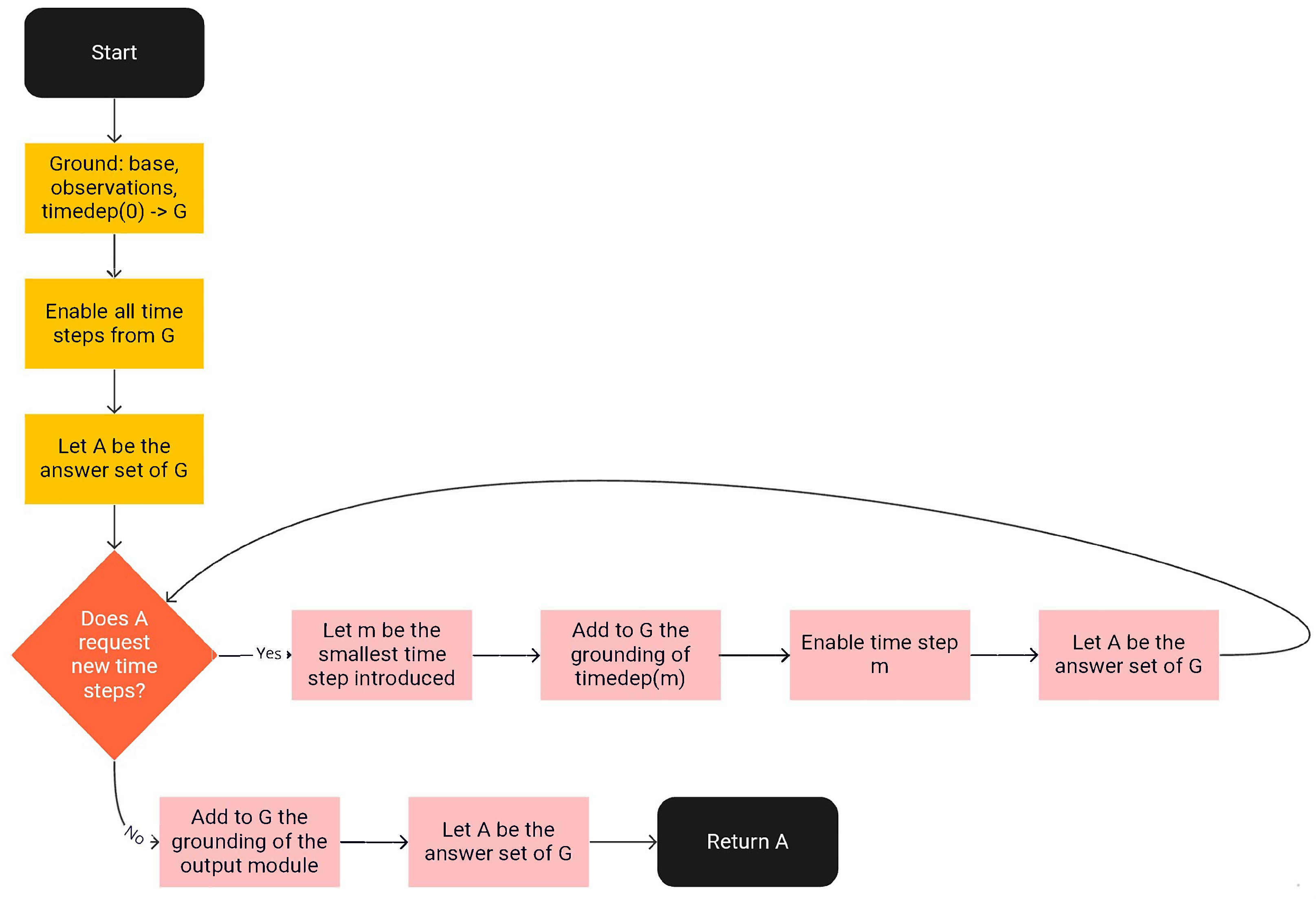
That is, is defined only if belongs to the part of timeline being considered. The above program is processed by Algorithm Incremental (Algorithm 2). A graphical depiction of the steps of the algorithm is also provided in Figure 1.
The algorithm leverages a fix-point computation to calculate a trajectory in an incremental fashion. The intuition is as follows. The algorithm takes as input a set of pre-determined time steps, e.g., corresponding to time steps that a user or external application would like to query about or about which observations are provided. Step 2 produces the grounding, G, of , p, O, and . Due to the fact that p defines the pre-determined time steps, ground instances of the rules of , which are time-dependent, are generated. Ground instances of external are also generated for every time step defined by p. Let us recall that externals are false by default: step 3 changes this by asserting all externals from G true via the corresponding clingo primitive. At step 4, the answer set A of G is computed. If A does not contain any request for new time steps, then A encodes the trajectory that Incremental aims at computing. Thus, all that is left is to ground incrementally (step 16) and return the answer set of the updated grounding (step 17).
| Algorithm 2 Algorithm Incremental |
|
On the other hand, if the answer set computed at step 4 contains requests for new times steps, then those requests need to be satisfied. Let us recall that the introduction of a new time step may affect the calculation of the state of the domain at the time steps that follow it. For this reason, the algorithm first finds the minimum requested time step, m (step 7). Next, step 9 adds the requested time step to G. Step 10 adds to G the groundings of all rules that compute the state of the domain at time steps m and later. Step 11 asserts and step 12 calculates the updated answer set A of G. At this point, the algorithm verifies whether A contains any requests for new time steps and the process repeats.
Let us now focus on the soundness and completeness of Algorithm Incremental with regard to the corresponding non-incremental way of computing the trajectory. To begin, we define the single-shot version of the program used by , which is obtained from by (a) removing all declarations, and (b) adding to each program the following rules:
The first statement assigns value 0 to constant t, thereby making all conditions of the form (from the pair of conditions ) trivially satisfied. The second statement ensures that every request for the introduction of a time step is immediately satisfied. The third statement ensures that all conditions of the form are satisfied whenever T represents a time step. We denote the single-shot version of a program by .
The soundness and completeness of Algorithm Incremental is thus given by the following theorem.
Theorem 1.
Given a program Π, set p of pre-determined time steps, and set O of observations, the trajectory encoded by Incremental coincides with the trajectory encoded by the answer set of clingo.
Proof.
Recall that the action descriptions considered are deterministic and strongly consistent, which means that clingo is guaranteed to return a single answer set. The claim can be proven by induction.
For the base case, one can note that, if the while loop of Incremental is never executed, then the computation carried out by Incremental is essentially equivalent to that carried out by clingo and thus the trajectories coincide. Along the same lines, if the set produced by clingo does not contain any literal formed by relation , then the while loop of Incremental is never executed and, once again, the trajectories encoded by the results of the two computations coincide.
For the inductive case, let us assume that the trajectories produced by the two algorithms share a (non-empty) prefix π and let us show that the next state in both trajectories (a) is associated with the same time step in both trajectories and (b) is the same in both cases. Let us begin with (a). Let and denote the time steps associated with the state that follows π, respectively, in the trajectory produced by Incremental and in that produced by clingo. Note that there must exist an iteration of the while loop of Incremental in which at step 7. By contradiction, suppose that . If that were the case, it would mean that the bodies of some rules of Π were satisfied at one or more time steps from π, and caused clingo to conclude for some t. Due to the fact that π is the shared prefix, then the bodies of same rules would have been satisfied during one of Incremental’s calls, yielding as well. However, if that were the case, would coincide with , which causes contradiction. Reasoning in a similar way, we can conclude that it is impossible that . Hence, . Furthermore, because the two time steps coincide, it is easy to see that the corresponding states must also be the same. □
5. Efficiency and Finity of Computations
One may notice that the incremental computation performed by Algorithm Incremental has a potential for being rather wasteful. In fact, of all the time steps that may have been potentially identified for addition, step 7 only takes one, essentially disregarding other requests for the addition of time steps that, if satisfied, could speed up the process rather substantially. In particular, it is not difficult to see that the number of iterations of the while loop is bound to be proportional to the length of the trajectory returned, which is undesirable when long trajectories are computed.
Additionally, one should note that action descriptions that contain durative fluents may sometimes yield infinite trajectories. To see how this may happen, consider fluents f, g and the corresponding information:
- f and g are default fluents;
- if f holds, then g holds for a duration of n units of time;
- if g is false, then f holds.
Suppose that f is observed to hold at step 0. Statement 2 causes g to hold until time step n. At step , g defaults to false and the condition of statement 3 becomes satisfied, causing f to hold. Again, item 2 causes g to hold until time step . At step , g defaults to false again and statement 3 causes f to hold. The same occurs again at . It is not difficult to see that the process repeats indefinitely, producing an infinite trajectory. Correspondingly, the Algorithm Incremental will yield infinite computations in these cases.
Central to overcoming this issue is the following simple but important observation on Algorithm Incremental:
Theorem 2.
Let be the value of m at step 7 of Incremental during a certain iteration of the while loop. At every subsequent iteration, the value of m is guaranteed to be no smaller than .
This property motivated the development of Incremental (Algorithm 3), shown below. Incremental aims at reducing the number of iterations necessary to compute a trajectory (at least in the average case) by taking into account a larger portion of the requests for the introduction of new time steps. Additionally, the algorithm takes as input an additional parameter h, which acts as a time horizon for the computation. Intuitively, the new algorithm terminates when all requests for new time steps at a given iteration are for time steps greater than h. Theorem 2 ensures that no requests for time steps smaller than h are missed in doing so.
The intuition is as follows. The algorithm takes as input a set of pre-determined time steps, e.g., corresponding to time steps that a user or external application would like to query about or about which observations are provided. Step 2 produces the grounding, G, of , p, and . Due to the fact that p defines the pre-determined time steps, ground instances of the rules of , which are time-dependent, are generated. Ground instances of external are also generated for every time step defined by p. Recall that externals are false by default: step 3 changes this by asserting all externals from G true via the corresponding clingo primitive. At step 4, the answer set A of G is computed. If A does not contain any request for new time steps, then A encodes the complete trajectory that Incremental aims at computing. Thus, all that is left is to ground incrementally (step 22) and return the answer set of the updated grounding (step 23).
On the other hand, if the answer set computed at step 4 contains requests for new times steps, then those requests need to be satisfied. Recall that the introduction of a new time step may affect the calculation of the state of the domain at the time steps that follow it. For this reason, the algorithm must retract all rules that are related to those time steps. This process begins with step 8, which finds the minimum requested time step, m.
If m is greater than the requested time horizon h, then the iterations terminate (step 10) and the computation is finalized (steps 22–23). Step 10 ensures the finity of the returned trajectories and, correspondingly, of the computation.
If , then step 10 removes from G the groundings of all rules that produce information about the state of the world at step m or greater. This is accomplished by setting the corresponding externals to false, which causes those rules to become inapplicable, and by releasing the externals. By releasing the externals, we ensure that, at steps 11 and 12, clingo will completely remove from G the groundings of all rules that have become inapplicable.
| Algorithm 3 Algorithm Incremental |
|
It is important to note that this retraction phase is a fundamental step in ensuring the satisfaction of the Module Theorem in Incremental. Without the retraction phase, it is not difficult to see that rules triggered during the following expansion phase may yield (ground) literals that are already derived by rules triggered at earlier time steps. This phenomenon is due to the presence of durative aspects in the action descriptions. If the language is restricted to traditional inertial and default fluents, then the retraction phase is not necessary.
Next, step 15 adds the requested time steps to G. Step 16 adds to G the groundings of all rules that compute the state of the world at time steps m and later. Step 17 asserts all externals from G true and step 18 calculates the updated answer set A of G. At this point, the algorithm verifies whether A contains any requests for new time steps and the process repeats.
One may want to notice that steps 10 and 17 result in the enabling of all time steps , i.e., of all newly introduced time steps as well as every time step that previously existed. The reason for enabling the latter set is that the retraction phase removes all information about the state of the domain at m and later time steps. During the following solving phase, the information must thus be recomputed. One may be tempted to think that this recomputation is unnecessary. However, this is not the case, because the state of domain at a previously existing time step t may be affected by changes occurring at a newly introduced time step that precedes t.
In comparing step 2–4, 10–12, and 16–18, one may observe that, when time steps greater than m are already present in the grounding at the time of steps 2–4, the corresponding rules are grounded and solved once at steps 2–4, then retracted at steps 10–12, and later regrounded and solved at steps 16–18. Undoubtedly, this process involves some degree of potential recomputation, but is necessary to ensure the satisfaction of the conditions of the Module Theorem. Retracting the rules is necessary to ensure that the necessary conditions are satisfied during the following expansion phase.
Rather than using , one may be tempted to introduce new time steps by means of a relation and correspondingly modified rule from (17):
However, this rule may in some cases lead to the violation of the conditions of the Module Theorem. To understand how this may happen, consider time steps greater than t and such that and are enabled (i.e., and both hold), and rules at both time steps require the introduction of time step (i.e., and both hold). Suppose that a retraction phase occurs (steps 8–12) to a time step m such that . In the following expansion phase (steps 15–18), the ASP program will effectively consist of two modules: a module containing ground rules corresponding to time steps 0 through , and a module containing ground rules corresponding to time steps m and greater. It is not difficult to see that each module contains a ground instance of the above definition of that defines . This violates the condition of the Module Theorem according to which . The use of relation in place of prevents this from happening, because module defines and module defines a different literal .
The soundness and completeness of Incremental are given by the following theorem.
Theorem 3.
Given a program Π, set p of pre-determined time steps, set O of observations, and time horizon h. If clingo terminates, then the trajectory encoded by Incremental coincides with the trajectory encoded by the answer set of clingo.
Proof.
The proof easily follows from Theorem 1. The key is to note that:
- At each iteration, Incremental is guaranteed to introduce at least the same time step introduced by Incremental;
- The retraction phase preserves all (ground) rules for time steps prior to m.
□
6. Experimental Evaluation
In order to evaluate the performance of Incremental, we compared its execution time against that of a single-shot (i.e., non-incremental) execution of clingo. To do this, we generated sets of observations about sequences of time steps of progressively increasing length from 1 to 114 steps, representing a typical test input for the user-facing application. Then, we ran the instances with both Incremental and clingo (in single-shot mode) in order to calculate the corresponding trajectories. The single-shot version of the program was obtained as described in Section 4.
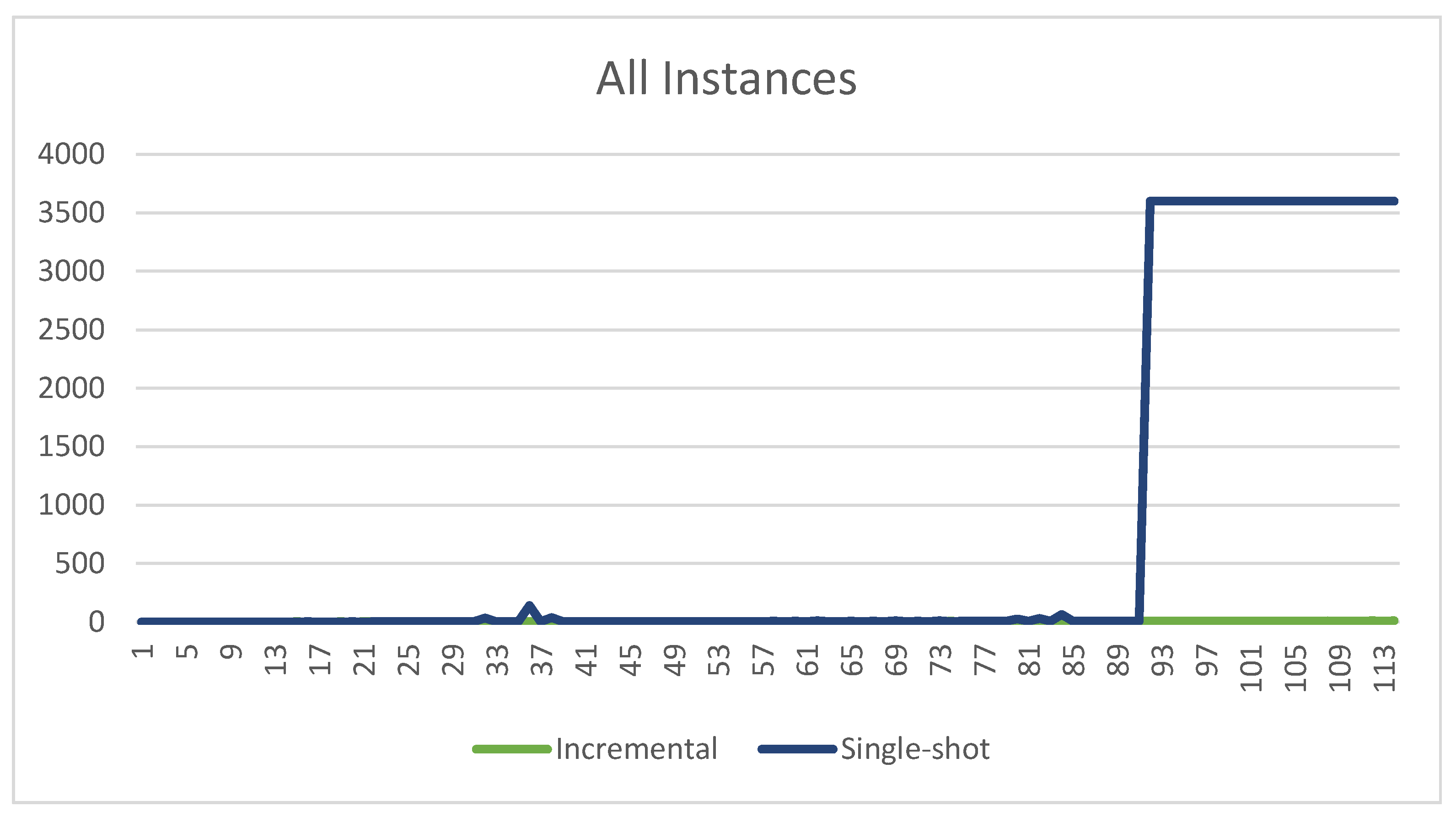
The experiments were executed on a computer running CentOS 7, equipped with an Intel Xeon CPU E5-2699 v3 at 2.30 GHz, 24 GB RAM, and using clingo 5.4.0, the version of clingo for whose incremental API Incremental was developed. Incremental was implemented in Python and configured as clingo’s control custom loop for the incremental runs. Every run was set up with a timeout of 1 h. The results are shown in Figure 2, Figure 3 and Figure 4.
Clingo in single-shot timed out 23 times out of 114, i.e., about 20% of the time. The average execution time of the instances that did not time out was s, with a standard deviation of and a maximum execution time of s. If one factors in the instances timed out, then the average time increased to s.
Incremental never timed out. The average execution time was within the requirements for practical use, with an average time of s, a standard deviation of , and a maximum execution time of s.
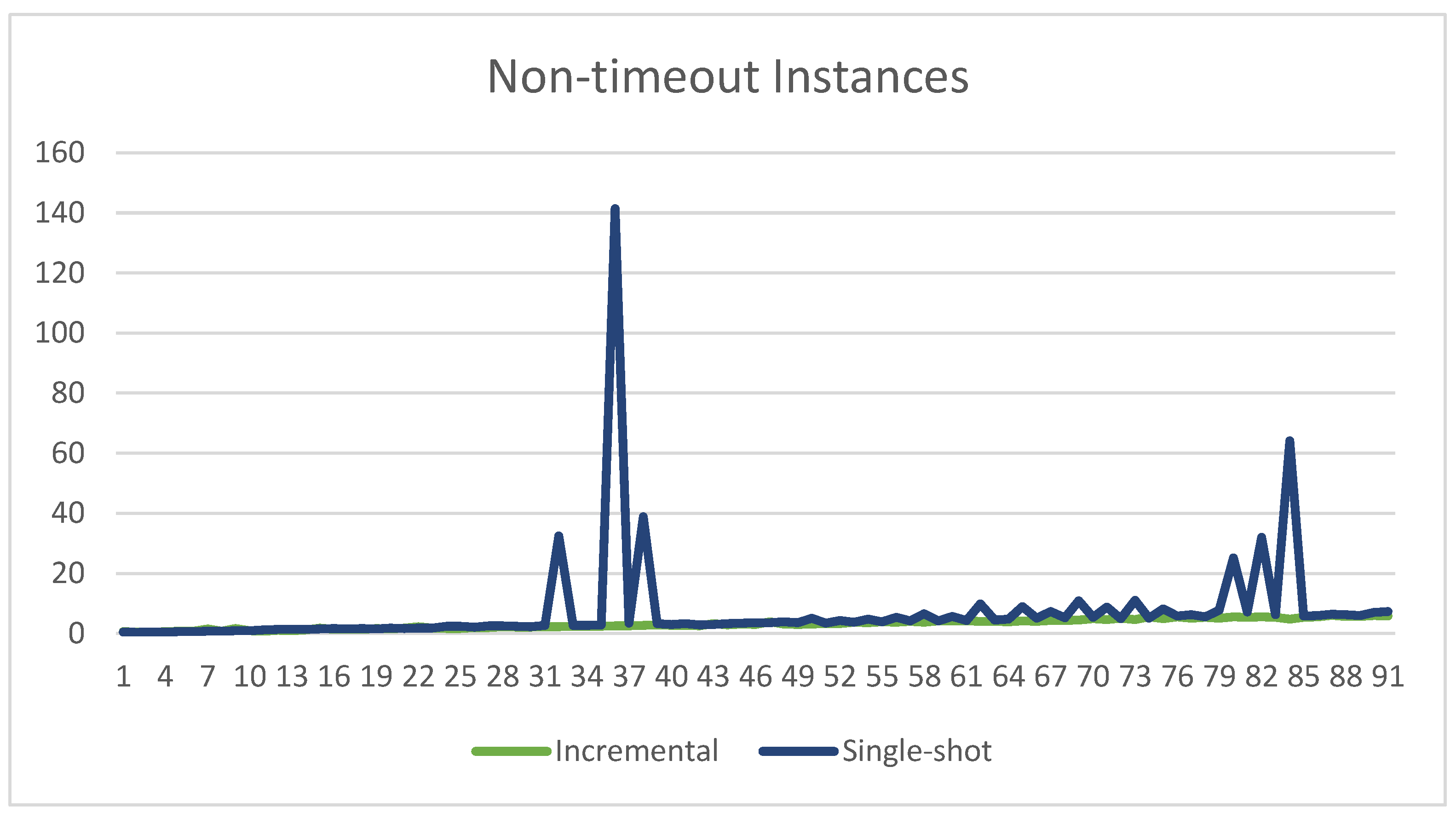
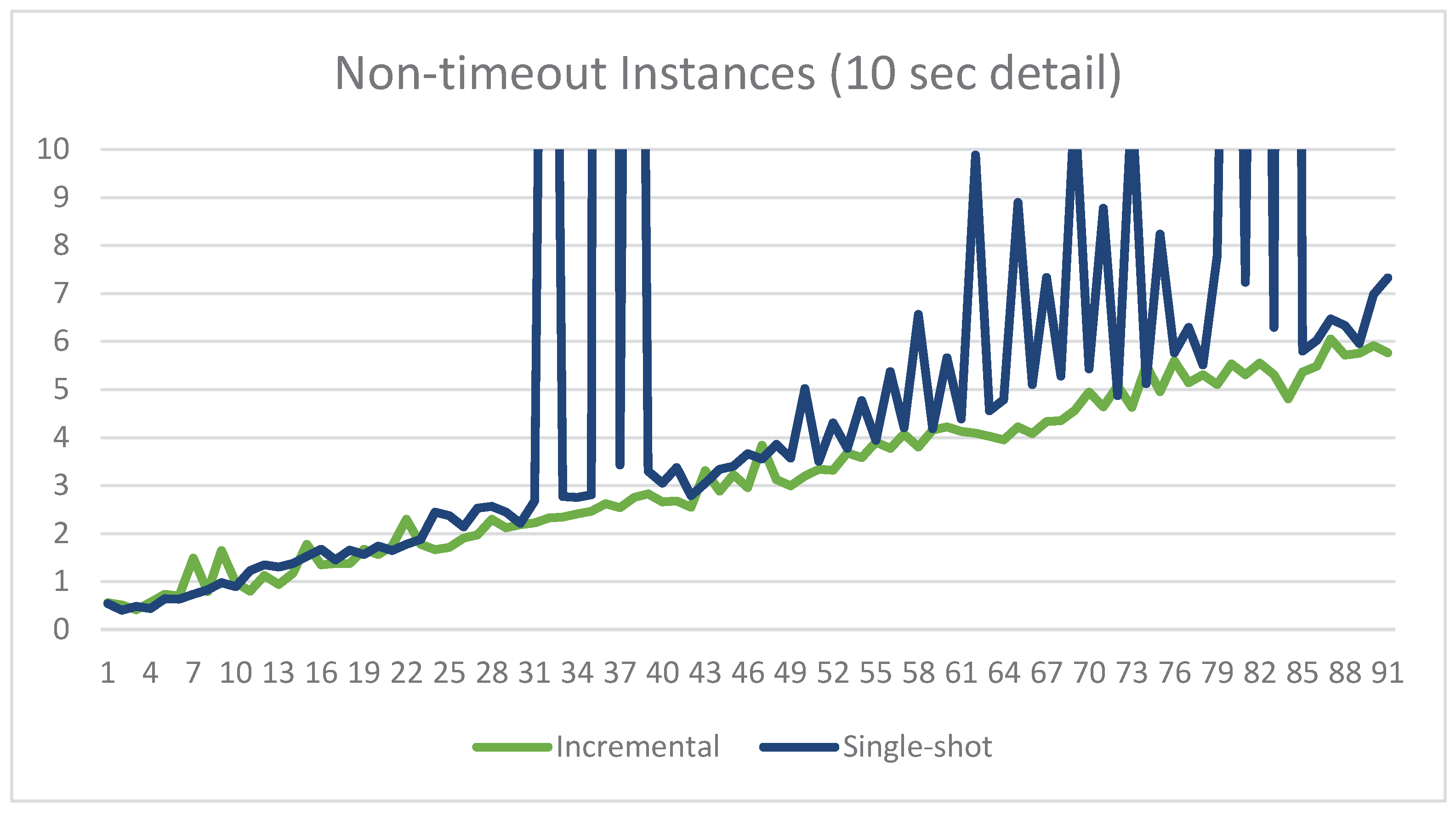
Comparing the performance of the two provides some clear indications of the greater consistency of Incremental. To begin with, the 23 timeouts of the single-shot version are of course extremely problematic for practical use. Incremental does not pose such an issue since it never timed out. Having said that, before the experimental phase of this project, we were unsure how Incremental would compare with the single-shot version on instances where the latter would not time out. In fact, Incremental involves a rather complex algorithm that is implemented in Python and runs as clingo’s control loop. The single-shot version, on the other hand, relies on clingo’s default control loop, which is written in highly optimized C/C++. On simpler instances, we suspected that the single-shot version may be faster. Furthermore, while indeed there is a number of simple instances in which the single-shot version is marginally faster, its performance rapidly degrades, as indicated by the higher values of average time ( s–or s!–vs. s), standard deviation ( vs. ), and substantially higher maximum execution time ( s vs. s). All in all, our experiments demonstrate the exceptional capabilities of clingo’s support for incremental computations, which enabled us to develop an ASP-based solution that featured consistently fast execution. The results also demonstrate the practical viability of our approach for extending the use of incremental computations to situations where straightforward encodings fail to satisfy the conditions of the Module Theorem.
An noteworthy observation on the single-shot instances that resulted in a time out is that, in all cases, the computation timed out during the grounding phase of the process. In fact, it would appear that, in those instances, the size of the grounding grows very dramatically, ultimately leading to either a time out or, if no time out is set, to an out-of-memory condition. We believe this to be an observation that has important implications on which other possible approaches are applicable to this problem. We comment on this topic in Section 10.
7. Practical Extensions: Accommodating Incremental Observations
In this and later parts of this paper, we focus on extensions of Algorithm Incremental (Algorithm 4) that are of practical interest.
One may observe that Algorithm Incremental (Algorithm 4) leverages clingo’s incremental infrastructure to improve performance for a given set of observations and queries. However, if further observations become available at a later time, the entire algorithm needs to be executed again. The refinement of Incremental shown below, called Incremental, can incrementally integrate observations as well. Incremental requires the output module to be modified to include a directive:
Additionally, every rule of the module must be expanded to include the condition . This modification enables Incremental to enable and disable the output module as needed.
| Algorithm 4 Algorithm Incremental |
|
Differently from Incremental, Incremental does not terminate and thus does not return any value. Rather, it assumes a two-way communication with the caller via primitives output and receive. The former is used to send an answer set to the caller and the latter is used to fetch a new set of observations from the caller. Incremental relies on the assumption that observations are never withdrawn, but while it is possible to lift this assumption, doing so is beyond the scope of this paper.
The overall flow of Incremental is as follows. At first, the algorithm is started and given a set of pre-determined time steps. These are used for the first iterative computation, which follows the same approach of Incremental, incrementally adding new time steps as prescribed by the durative state constraints of the program. At the end of that computation, the output module is added and the corresponding answer set sent to the caller (step 34). Then, the algorithm waits for new observations (step 36). When those are received, the output module is removed from the program (step 37), since its conclusions will need to be completely reevaluated later. Then, the smallest time step m among those of the new observations is found (step 38). This step assumes the existence of a function that returns the time step of the observation provided to it. The algorithm, then, returns to step 13, where a retraction phase occurs, aimed at removing from the program all rules related to time step m and later time steps. Following this, the computation follows the same flow of Incremental, eventually resulting in an updated answer set being passed to the caller at step 34, after which Incremental returns to waiting for new observations.
8. Computation from a Saved State
While Incremental often makes it possible to efficiently incorporate new observations, it has two potential drawbacks:
- If the observations receive require backtracking to a much earlier time step, the resulting computation may be slow. In our experiments, we observed instances in which the algorithm took about 20 s for computing the states corresponding to a timeline that contained observations for a certain collection of time steps, while the algorithm was able to complete the computation in about 8 s when provided all relevant time steps at the beginning of the computation.
- Incremental stores the information about the search space in memory. Thus, the use of Incremental+ may not be feasible on cloud platforms where service instances are frequently terminated (possibly without warning) and restarted.
Thus, in this section we discuss a different approach, in which we build once again upon Algorithm Incremental to make it possible to efficiently resume the computation from a saved state. This approach relies on a slight modification of Algorithm Incremental, called Algorithm Incremental, which takes an additional input argument s, which is a set of facts encoding a previously saved state of the domain. The facts include not only information about which fluents literals are true in that state, but also (a) information about the amount of time left for durative fluents and (b) facts of the form for any future time step that needs to be considered in the evaluation of the behavior of durative fluents. The algorithm also assumes that the time step of s is included in input argument p. Step 2 of Incremental is modified as follows:
that is, s is included in the initial grounding process. The entire list of steps of Algorithm Incremental is not given due to the simplicity of the modifications.
Rather than always starting its computation from scratch, Incremental is capable of beginning its computation from a previously computed state of the domain. The algorithm builds upon the observation that, even in the presence of durative fluents, every state of a trajectory depends solely on the state that precedes it (as well as any actions that may occur in it). Therefore, executing Incremental on a previously saved state does not hinder the correctness of its computation. The soundness and completeness of Incremental with regard to Incremental is ensured by the following property:
Lemma 1.
Let be the time step of saved state s. The value of m at step 8 of Incremental (refer to the same-numbered step of Algorithm 3) is guaranteed to be greater than .
Incremental is leveraged by Algorithm 5, shown below.
| Algorithm 5 Algorithm UpdateCache |
|
The algorithm relies on the assumption that the user maintains a record of the latest saved trajectory as well as of all previously received observations. When new observations become available, the user invokes UpdateCache. Then, UpdateCache determines the smallest time step that is affected by the new observations and incrementally updates the remaining part of the trajectory, returning the result of the computation. Intuitively, the trajectory will then be saved by the user for later reuse, when new observations are received.
It is not difficult to see that the algorithm can seamlessly handle cases in which earlier parts of the trajectory are missing, e.g., if they have been dropped to save memory. If new observations correspond to states that pre-date the first state of the trajectory, UpdateCache falls back to recomputing the trajectory from scratch using the record of all observations.
Due to these features, UpdateCache is suitable for use on cloud platforms where nodes may be terminated and restarted, as well as in cases in which memory constraints prevent one from saving a complete trajectory. Under those conditions, UpdateCache is still capable of leveraging clingo’s incremental computation capabilities and of avoiding recomputations whenever possible.
9. Related Work
We already discussed the literature that is conceptually closest to our work, namely [19], which explored mechanisms for handling “wall-clock” time in the context of action languages and ASP-based domain representations, and [21], where additive fluents were investigated. The body of literature on linear temporal logics (LTLs) [24,25] is also relevant to the representation and reasoning about “wall-clock” time. Particularly interesting are the line of research on linear dynamic logic on finite traces (LTLf) [26,27,28], as well as the integration of LTLs with ASP [29], but while all of these approaches provide useful and convenient solutions to the representational problem related to “wall-clock” time, it is not immediately clear whether they provide a solution to the computational problem that we faced.
More closely related to our computational problem is the recent work on overgrounding [30]. Overgrounding provides a “ground-once-solve-many” approach for the efficient processing of a continuous stream of data by limiting the number of times the corresponding ASP program is grounded. There are two important aspects that, in our opinion, limit the potential applicability of overgrounding to the problem at hand. First of all, overgrounding is most appropriate for a stream of data in which the new data is about more recent time points than the prior data. In our case, the new data may be about past time points, e.g., newly received information about tests (or exposure) that occurred in the past. Second, as we noted in Section 6, in the instances that are problematic for single-shot solving, it is the grounding process that times out due to a dramatic growth of the grounding of the program. Since overgrounding essentially relies on building a larger grounding than needed in order to accommodate future inputs without further grounding, it is difficult to see how the overgrounding technique may help address the performance issues that motivated our work without major modifications.
It is worth pointing out that research has been recently conducted at the intersection of ASP and high-utility pattern mining (HUPM). The work in [31] describes an approach that lifts the typical assumption according to whcih each item of a knowledge base is associated with a single utility. It is conceivable that approaches of this kind may provide insights into alternate techniques for improving efficiency in the context of the problems considered in this paper. Additionally, it may be interesting to investigate how HUPM may be leveraged go beyond the reasoning task considered here, and particularly for mining the data received by the system and identify potentially relevant patterns, such as unexpected virus propagation pathways.
Finally, other solvers with multi-shot capabilities have been recently released, e.g., [8]. An investigation on the relationship between our techniques and the multi-shot computation capabilities provided by these solvers is certainly important, but beyond the scope of the present paper.
10. Conclusions
Incremental techniques aim at making it possible to improve the performance of the grounding and solving processes by reusing the results of previous executions. ASP solver clingo supports both incremental grounding and incremental solving computations. In order to leverage incremental computations in clingo, the modules of ASP programs must satisfy certain safety-related conditions related to the Module Theorem. In a number of problem domains and reasoning tasks, these conditions can be satisfied in a fairly straightforward way. However, in certain practical applications, satisfying the conditions becomes more challenging, to the point that it is sometimes unclear how or even if it is possible to leverage incremental computations.
In this paper, we reported on our success in leveraging clingo’s support for incremental computations in one such practical application, where ASP was used for formalizing and reasoning about COVID-19 policies. Generally speaking, the task of focus was that of calculating the trajectories of dynamic domains in the presence of durative aspects, such as (default) durative fluents. This paper discussed a number of algorithms that we developed to enable the use of incremental computations in these situations in which straightforward encodings do not seem to be viable due to the constraints of the Module Theorem. Our experimental evaluation showed that our approach allows one to leverage incremental computations in an effective way, yielding substantially improved performance and a substantially improved ability to consistently produce a result within a reasonable amount of time regardless of the complexity of the trajectory being computed.
In terms of concrete contributions, our paper provided an approach for representing dynamic domains that are suitable for incremental techniques despite the presence of durative components, algorithms that leverage clingo’s incremental computation capabilities and avoid problems related to the conditions of the Module Theorem, and a demonstration of the substantial advantages of these algorithms over non-incremental approaches when it comes to efficiency of computation. Our results confirm the exceptional capabilities of clingo’s incremental computations and demonstrate that restrictions on the use of such features can be overcome with suitable representation techniques and algorithms.
While our approach provides an efficient way for addressing the domains discussed in this paper, there are two potential limitations that we have identified, and that are worth considering. Upon inspection of the use of the retraction and expansion phases in Algorithm Incremental, one can see that there is a worst-case scenario in which the retraction phase removes all time points added by the previous expansion phase but one. In those cases, one would be better off using Algorithm Incremental instead. The other limitation was already discussed in Section 6: Incremental, at least in its current form, is fairly computationally heavy compared to the default control loop in clingo. As a result, in particularly simple instances, the single-shot version may outperform Incremental, although in our experiments the single-shot version was never more than marginally faster. Overcoming these potential limitations will be the subject of future research. We also plan to conduct a more thorough experimental evaluation spanning over multiple domains.
Author Contributions
Conceptualization, M.B. (Marcello Balduccini) and M.B. (Michael Barborak); methodology, M.B. (Marcello Balduccini) and M.B. (Michael Barborak); software, M.B. (Marcello Balduccini) and M.B. (Michael Barborak); validation, M.B. (Marcello Balduccini), M.B. (Michael Barborak) and D.F.; formal analysis, M.B. (Marcello Balduccini); investigation, M.B. (Marcello Balduccini), M.B. (Michael Barborak) and D.F.; resources, D.F.; data curation, M.B. (Marcello Balduccini) and M.B. (Michael Barborak); writing—original draft preparation, M.B. (Marcello Balduccini) and M.B. (Michael Barborak); writing—review and editing, M.B. (Michael Barborak); visualization, M.B. (Michael Barborak); supervision, D.F.; project administration, D.F.; funding acquisition, D.F. All authors have read and agreed to the published version of the manuscript.
Funding
This research received no external funding.
Data Availability Statement
Not applicable.
Conflicts of Interest
The authors declare no conflict of interest.
References
- Gelfond, M.; Lifschitz, V. Classical Negation in Logic Programs and Disjunctive Databases. New Gener. Comput. 1991, 9, 365–385. [Google Scholar] [CrossRef] [Green Version]
- Marek, V.W.; Truszczynski, M. Stable Models and an Alternative Logic Programming Paradigm. In The Logic Programming Paradigm: A 25-Year Perspective; Springer: Berlin/Heidelberg, Germany, 1999; pp. 375–398. [Google Scholar]
- Falkner, A.; Friedrich, G.; Schekotihin, K.; Taupe, R.; Teppan, E.C. Industrial Applications of Answer Set Programming. KI–Kunstl. Intell. 2018, 32, 165–176. [Google Scholar] [CrossRef] [Green Version]
- Balduccini, M.; Gelfond, M.; Nogueira, M. Answer Set Based Design of Knowledge Systems. Ann. Math. Artif. Intell. 2006, 47, 183–219. [Google Scholar] [CrossRef] [Green Version]
- Gebser, M.; Kaufmann, B.; Neumann, A.; Schaub, T. Conflict-Driven Answer Set Solving. In Proceedings of the Twentieth International Joint Conference on Artificial Intelligence (IJCAI’07), Hyderabad, India, 6–12 January 2007; pp. 386–392. [Google Scholar]
- Kaminski, R.; Schaub, T.; Wanko, P. A Tutorial on Hybrid Answer Set Solving with Clingo. In Proceedings of the Thirteenth International Summer School of the Reasoning Web (RW-2017), London, UK, 7–11 July 2017; pp. 167–203. [Google Scholar]
- Gebser, M.; Kaminski, R.; Kaufmann, B.; Schaub, T. Multi-shot ASP Solving with Clingo. J. Theory Pract. Log. Program. (TPLP) 2019, 19, 27–82. [Google Scholar] [CrossRef] [Green Version]
- Calimeri, F.; Ianni, G.; Pacenza, F.; Perri, S.; Zangari, J. ASP-Based Multi-Shot Reasoning via DLV2 with Incremental Grounding. In Proceedings of the Fourteenth International Symposium on Practical Aspects of Declarative Languages (PADL 2012), Philadelphia, PA, USA, 23–24 January 2012; Number 7149 in Lecture Notes in Artificial Intelligence (LNCS). Russo, C., Zhou, N.F., Eds.; Springer: Berlin/Heidelberg, Germany, 2012; pp. 1–9. [Google Scholar]
- Oikarinen, E.; Janhunen, T. Modular Equivalence for Normal Logic Programs. In Proceedings of the Seventeenth European Conference on Artificial Intelligence (ECAI’06), Riva del Garda, Italy, 1 September 2006; pp. 412–416. [Google Scholar]
- Janhunen, T.; Oikarinen, E.; Tompits, H.; Woltran, S. Modularity Aspects of Disjunctive Stable Models. J. Artif. Intell. Res. 2009, 35, 813–857. [Google Scholar] [CrossRef]
- Gelfond, M.; Lifschitz, V. Action Languages. Electron. Trans. AI 1998, 3, 193–210. [Google Scholar]
- Baral, C.; Gelfond, M. Reasoning Agents in Dynamic Domains. In Logic-Based Artificial Intelligence; Springer: Boston, MA, USA, 2000; pp. 257–279. [Google Scholar]
- Balduccini, M. People, Ideas, and the Path Ahead. In Proceedings of the 24th International Symposium on Practical Aspects of Declarative Languages (PADL 2022), Philadelphia, PA, USA, 17–18 January 2022; Lecture Notes in Artificial Intelligence (LNCS). 2022; Volume 13165. [Google Scholar]
- Available online: https://www.billboard.com/pro/super-bowl-halftime-show-covid-safety-coronavirus/ (accessed on 10 January 2023).
- Available online: https://www.cdc.gov/coronavirus/2019-ncov/community/guidance-business-response.html (accessed on 10 January 2023).
- McCarthy, J. Programs with Common Sense. In Proceedings of the Teddington Conference on the Mechanization of Thought Processes, London, Her Majesty’s Stationary Office. 1959, pp. 75–91. Available online: https://books.google.com.hk/books?hl=zh-CN&lr=&id=ig8mHog30X0C&oi=fnd&pg=PA54&dq=%7BPrograms+with+%7BCommon+%7BSense.&ots=fmkH502LFW&sig=Bvb--R1ln9kYZ8TMMEG2lWg0_pI&redir_esc=y#v=onepage&q=%7BPrograms%20with%20%7BCommon%20%7BSense.&f=false (accessed on 10 January 2023).
- Hayes, P.J.; McCarthy, J. Some Philosophical Problems from the Standpoint of Artificial Intelligence. In Machine Intelligence 4; Meltzer, B., Michie, D., Eds.; Edinburgh University Press: Edinburgh, UK, 1969; pp. 463–502. [Google Scholar]
- Balduccini, M. Answer Set Based Design of Highly Autonomous, Rational Agents. Ph.D. Thesis, Texas Tech University, Lubbock, TX, USA, 2005. [Google Scholar]
- Chintabathina, S.; Watson, R. A New Incarnation of Action Language H. In Logic Programming, Knowledge Representation, and Nonmonotonic Reasoning: Essays Dedicated to Michael Gelfond on the Occasion of His 65th Birthday; Balduccini, M., Son, T.C., Eds.; Lecture Notes in Artificial Intelligence (LNCS); Springer: Berlin/Heidelberg, Germany, 2011; pp. 560–575. [Google Scholar]
- Balduccini, M.; Lierler, Y. Constraint Answer Set Solver EZCSP and Why Integration Schemas Matter. J. Theory Pract. Log. Program. (TPLP) 2017, 17, 462–515. [Google Scholar] [CrossRef] [Green Version]
- Lee, J.; Lifschitz, V. Additive Fluents. In Proceedings of the Answer Set Programming: Towards Efficient and Scalable Knowledge Representation and Reasoning, Stanford, CA, USA, 26–28 March 2001. [Google Scholar]
- Balduccini, M.; Gelfond, M. Diagnostic reasoning with A-Prolog. J. Theory Pract. Log. Program. (TPLP) 2003, 3, 425–461. [Google Scholar] [CrossRef] [Green Version]
- McCain, N. Causality in Commonsense Reasoning about Actions. Ph.D. Thesis, University of Texas, Austin, TX, USA, 1997. [Google Scholar]
- Kamp, J. Tense Logic and the Theory of Linear Order. Ph.D. Thesis, University of California, Los Angeles, CA, USA, 1968. [Google Scholar]
- Pnueli, A. The Temporal Logic of Programs. In Proceedings of the 18th Annual Symposium on Foundations of Computer Science, Providence, RI, USA, 31 October–2 November 1977; pp. 46–57. [Google Scholar]
- Giacomo, G.D.; Vardi, M. Linear temporal logic and linear dynamic logic on finite traces. In Proceedings of the Twenty-Third International Joint Conference on Artificial Intelligence, Beijing China, 3–9 August 2013. [Google Scholar]
- Giacomo, G.D.; Stasio, A.D.; Fuggitti, F.; Sasha, R. Pure-Past Linear Temporal and Dynamic Logic on Finite Traces. In Proceedings of the Twenty-Ninth International Joint Conference on Artificial Intelligence, Yokohama, Japan, 7–15 January 2020; pp. 4959–4965. [Google Scholar]
- Giacomo, G.D.; Murano, A.; Patrizi, F.; Perelli, G. Timed Trace Alignment with Metric Temporal Logic over Finite Traces. In Proceedings of the 18th International Conference on Principles of Knowledge Representation and Reasoning, Online, 3–12 November 2021; pp. 227–236. [Google Scholar]
- Aguado, F.; Aguado, F.; Dieguez, M.; Perez, G.; Schaub, T.; Schuhmann, A.; Vidal, C. Linear-Time Temporal Answer Set Programming. J. Theory Pract. Log. Program. (TPLP) 2023, 23, 2–56. [Google Scholar] [CrossRef]
- Calimeri, F.; Ianni, G.; Pacenza, F.; Perri, S.; Zangari, J. Incremental Answer Set Programming with Overgrounding. J. Theory Pract. Log. Program. (TPLP) 2019, 19, 957–973. [Google Scholar] [CrossRef] [Green Version]
- Cabalar, P.; Terracina, G. An Answer Set Programming Based Framework for High-Utility Pattern Mining Extended with Facets and Advanced Utility Functions. In Proceedings of the Rules and Reasoning: 5th International Joint Conference (RuleML + RR 2021), Online, 8–15 September 2021; pp. 13–15. [Google Scholar]
Figure 1.
Graphical depiction of the steps of Incremental.

Figure 2.
Comparison of the execution times for all instances.

Figure 3.
Comparison of the execution times for all instances that did not time out.

Figure 4.
Comparison of the execution times for all instances that did not time out, 0–10 s detail.

Disclaimer/Publisher’s Note: The statements, opinions and data contained in all publications are solely those of the individual author(s) and contributor(s) and not of MDPI and/or the editor(s). MDPI and/or the editor(s) disclaim responsibility for any injury to people or property resulting from any ideas, methods, instructions or products referred to in the content. |
© 2023 by the authors. Licensee MDPI, Basel, Switzerland. This article is an open access article distributed under the terms and conditions of the Creative Commons Attribution (CC BY) license (https://creativecommons.org/licenses/by/4.0/).
Share and Cite
MDPI and ACS Style
Balduccini, M.; Barborak, M.; Ferrucci, D. Pushing the Limits of Clingo’s Incremental Grounding and Solving Capabilities in Practical Applications. Algorithms 2023, 16, 169. https://doi.org/10.3390/a16030169
AMA Style
Balduccini M, Barborak M, Ferrucci D. Pushing the Limits of Clingo’s Incremental Grounding and Solving Capabilities in Practical Applications. Algorithms. 2023; 16(3):169. https://doi.org/10.3390/a16030169
Chicago/Turabian StyleBalduccini, Marcello, Michael Barborak, and David Ferrucci. 2023. "Pushing the Limits of Clingo’s Incremental Grounding and Solving Capabilities in Practical Applications" Algorithms 16, no. 3: 169. https://doi.org/10.3390/a16030169
Note that from the first issue of 2016, this journal uses article numbers instead of page numbers. See further details here.