Article

Nearest Neighbours Graph Variational AutoEncoder

by
Lorenzo Arsini
1,2,
Barbara Caccia
3,
Andrea Ciardiello
2,*,
Stefano Giagu
1,2,* and
Carlo Mancini Terracciano
1,2
1
Department of Physics, Sapienza University of Rome, 00185 Rome, Italy
2
INFN Section of Rome, 00185 Rome, Italy
3
Istituto Superiore di Sanità, 00161 Rome, Italy
*
Authors to whom correspondence should be addressed.
Algorithms 2023, 16(3), 143; https://doi.org/10.3390/a16030143
Submission received: 20 December 2022 / Revised: 7 February 2023 / Accepted: 28 February 2023 / Published: 6 March 2023
(This article belongs to the Special Issue Deep Learning Architecture and Applications)

Abstract

:
Graphs are versatile structures for the representation of many real-world data. Deep Learning on graphs is currently able to solve a wide range of problems with excellent results. However, both the generation of graphs and the handling of large graphs still remain open challenges. This work aims to introduce techniques for generating large graphs and test the approach on a complex problem such as the calculation of dose distribution in oncological radiotherapy applications. To this end, we introduced a pooling technique (ReNN-Pool) capable of sampling nodes that are spatially uniform without computational requirements in both model training and inference. By construction, the ReNN-Pool also allows the definition of a symmetric un-pooling operation to recover the original dimensionality of the graphs. We also present a Variational AutoEncoder (VAE) for generating graphs, based on the defined pooling and un-pooling operations, which employs convolutional graph layers in both encoding and decoding phases. The performance of the model was tested on both the realistic use case of a cylindrical graph dataset for a radiotherapy application and the standard benchmark dataset sprite. Compared to other graph pooling techniques, ReNN-Pool proved to improve both performance and computational requirements.

1. Introduction

Deep Generative Modeling involves training a deep neural network to approximate the high-dimensional probability distribution of the training data, enabling the generation of new examples from that distribution. There are various approaches to deep generative modeling, such as Generative Adversarial Networks (GANs) [1], Variational AutoEncoders (VAEs) [2], and Normalizing Flow models [3]. A comprehensive review of deep generative modeling can be found in [4].
In some cases, the architecture includes both an encoding and a decoding scheme, as is the case with models such as VAEs. The encoding process is typically used to obtain compact representations of the data distribution, often achieved through pooling operations that reduce the dimensionality of the data. The creation of a “bottleneck” by embedding the input samples in lower and lower dimensional spaces enables the extraction of essential features of the data. The decoding scheme, on the other hand, often employs reverse techniques used in the encoding, such as un-pooling operations, to restore the original dimensionality of the data.
In recent years, there has been a growing interest in utilizing Deep Learning in the field of Medical Physics. Specifically, in Radiotherapy (RT), Deep Generative modeling presents a valuable opportunity to streamline the calculation of deposited dose distributions by radiation in a given medium. These data, which are currently computed using more resource-intensive methods, can be utilized to optimize and validate RT treatment plans. Little effort has been made so far in this area, except for in the works of [5,6]. Models for this application should possess two key properties. Firstly, a high resolution in dose prediction is crucial and requires the ability to process large data efficiently. Secondly, models should be lightweight to enable their use in resource-constrained medical devices and for online training. In the future, real-time imaging may enable real-time treatment planning optimization, making it imperative to use fast Deep Learning models during both training and inference.
Deep Learning applications can find a role in specialised hardware for both resource efficient deployment and fast inference tasks. These models are referred to as Lightweight models and they are designed to be small and efficient, making them well-suited for use on resource-constrained devices. Notable applications are embedded software in Internet of Things (IoT) devices [7], wearable medical devices [8], and real-time applications such as online video analysis, e.g., online crowd control [9]. A similar need is also present for models developed for fast inference on accelerated hardware, for which a keypoint example is the trigger analysis in high energy physics experiments [10]. These models are typically smaller and less complex than traditional deep learning models, which allow them to run on devices with limited computational power and memory. Moreover, designing them often involves trade-offs between computational resources and performance.
Deep Generative Modeling is commonly based on Convolutional Neural Networks (CNNs) for many applications, as they are one of the most powerful tools for processing grid-like data in Deep Learning frameworks. However, a significant amount of real-world data is better described by more flexible data structures, such as graphs.
A graph is defined by a pair G = ( V , E ) . V = { v i } i = 1 N is a set of N vertices, or nodes, while E = { e i j } i , j = 1 N is the set of edges, which carry the relational information between nodes. The edge set E can be organised into the adjacency matrix A, an N x N binary matrix, whose elements A i j are equal to 1 if a link between i-th and j-th node exists and is equal to 0 otherwise.
To address learning tasks on graphs, there has been an increasing interest in Graph Neural Networks (GNNs). These architectures typically use Graph Convolutional layers (GCNs), which allow for the processing of data on graphs, generalizing the concept of convolutions in CNNs. There are currently several types of GCNs available, ranging from the simplest models [11,12], to those based on graph spectral properties [13], and those that include attention mechanisms [14]. Although it is currently possible to achieve excellent results in solving various problems of classification, regression, or link prediction on graphs, graph generation remains an open challenge [15].
Unlike images, graphs often have complex geometric structures that are difficult to reproduce, particularly in an encoder–decoder framework. Despite various approaches existing, there is currently no standard method for addressing this class of problems. Standard classes of models for graph generation are Graph AutoEncoders (GAEs) and Variational Graph AutoEncoders (VGAEs) [16], which apply the concepts of AutoEncoders and Variational AutoEncoders (VAEs) to graphs. However, these architectures can only reconstruct or generate the adjacency matrix of the graphs, not the features of their nodes. Additionally, while these models can learn meaningful embeddings of node features, the graph structure and number of nodes remain fixed during the encoding process, resulting in no compression of input data through pooling operations and no bottleneck.
Different strategies have been developed for pooling operations on graphs. Early works used the eigen-decomposition for graph coarsening operations based on the graph topological structure, but these methods are often computationally expensive. An alternative algorithm is the Graclus algorithm [17], used in [13] and later adopted in other works on GNNs. Approaches like this aim to define a clustering scheme on graphs, on top of which it is possible to apply a standard max or mean pooling. Other approaches, such as SortPooling [18], select nodes to pool based on their importance in the network. There is also a stream of literature that bases pooling operations on spectral theory [19,20]. Finally, state-of-the-art approaches rely on learnable operators that, such as message-passing layers, can adapt to a specific task to compute the optimal pooling, such as DiffPool [21], Top-K pooling [22], and ASAPooling [23]. These pooling methods have been demonstrated to perform well when integrated into GNN models for graph classification, but all have limitations. For example, DiffPool learns a dense matrix to assign nodes to clusters, thus it is not scalable to large graphs. Top-k pooling samples the top-k aligned nodes with a learnable vector, not considering the graph connectivity. In this way, after the pooling, a good connectivity between the surviving nodes is not guaranteed. ASAPooling uses a self-attention mechanism for cluster formation and a top-k scoring algorithm for cluster selection, also taking into account graph connectivity. While overcoming some limitations of previous methods, this pooling requires more computations, which can lead to high computing needs for large graphs.
In contrast to pooling procedures, there is currently a lack of solutions for un-pooling operations for graphs that can be considered the inverse of pooling. The only works that attempt to define such operations are described in [22,24]. Other decoding schemes for graph generation are designed in different ways, most of which are task-specific. For example, in many algorithms for protein or drug structure generation, decoding is conducted by adding nodes and edges sequentially [25,26]. On the other hand, there are also works on “one-shot” graph generation, with decoding architectures that can output the node and edge features in a single step [27,28]. However, in various works that use this approach, the decoding of nodes and edges are considered separately and do not take into account the structure of the graphs. For example, in [29], a 1D-CNN is used to decode node features and a 2D-CNN is used for edge features.
In summary, we found that the current literature lacks:
  • A pooling operation for graph data that takes into account graph connectivity and, at the same time, is lightweight and scalable to a large graph;
  • A graph generative model based on an encoder–decoder architecture;
  • A decoding solution that is based on the message passing algorithm.
In this study, we propose a model for graph generation based on Variational AutoEncoders. We focus on the case of graph data with a fixed, regular, and known geometric structure. To this end, we have developed:
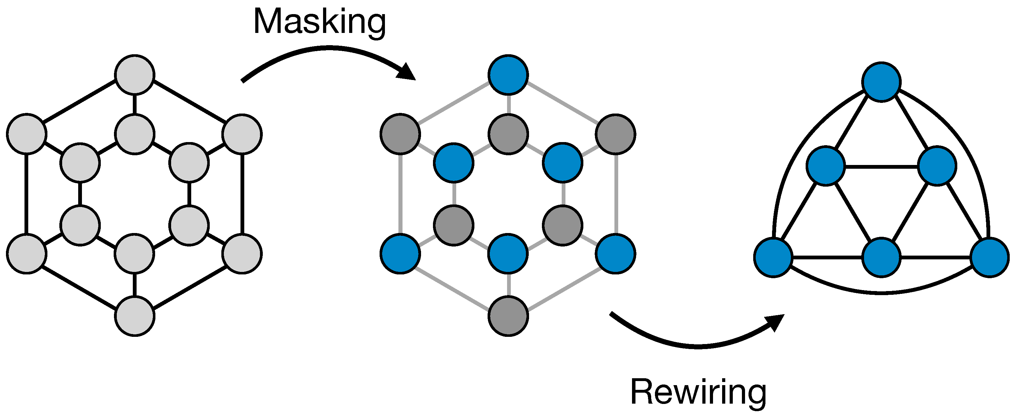
  • Simple, symmetrical, and geometry-based pooling and unpooling operations on graphs, which allow for the creation of bottlenecks in neural network architectures and that are scalable to large graphs;
  • A Variational AutoEncoder for regular graph data, where both the encoding and decoding modules use graph convolutional layers to fully exploit the graph structure during the learning process.
The remainderof the study is organized as follows. In Section 2, we describe our proposed deep learning architecture and the datasets used. First, in Section 2.1, we introduce our Nearest Neighbors Graph VAE, describing how the developed pooling and unpooling techniques work and how they are integrated into the generative model. Then, in Section 2.2, we describe the benchmark sprite dataset and present our own set of cylindrical-shaped graph data for a Medical Physics application. In Section 3, we present the results of applying our Graph VAE to the described datasets. We also conduct an ablation study to compare the performance of our model using different pooling and unpooling techniques. The paper concludes with a final discussion in Section 4.

2. Materials and Methods

2.1. Nearest Neighbour Graph VAE

In this section, we introduce our Nearest Neighbour Graph VAE model, which uses graph convolutions in both the encoding and decoding operations. To create a bottleneck in the architecture, we propose new symmetrical graph pooling and un-pooling techniques, which we refer to as Recursive Nearest Neighbour Pooling and Un-Pooling (ReNN-Pool and Un-Pool). Such operations enable the construction of a VAE decoder based on graph convolutions.

2.1.1. ReNN-Pool and Un-Pool

In CNNs, pooling operations are widely used to decrease the dimensionality of feature maps while increasing the receptive fields of neurons when processing grid-like data. This is easily possible on images, where a standard pooling layer typically involves a downsampling operation such as the max or mean function applied to groups of nearby pixels. Conversely, applying this idea to graph structures is generally a challenging task.
However, there are cases where, although data does not have a grid-like shape and can be better processed with GNNs, the graph structures are fixed and have a regular and known geometry. For example, some datasets may contain examples whose data are arranged in a cylindrical or spherical structure. For these cases, we developed a simple pooling operation (ReNN-Pool) that can sub-sample graph nodes in a regular way.
The ReNN-Pool consists in a masking operation and a subsequent update of the adjacency matrix of the graph. First of all, nodes are sorted on the basis of their position in the graph. For example, if samples have a cylindrical structure, nodes can be hierarchically ordered on the basis of their positions along the z, θ and r axes. Then, the masking operation is carried out. Masking consists in dropping, i.e., removing, certain nodes from the graph. The process is performed in a recursive manner on the sorted node list. It begins with the first node, which is preserved, while all its nearest neighbours are dropped and removed from the node list. The process then continues with the next node and repeats, until all nodes in the list have been processed.
After the masking, we rewire links between the “survived” nodes, connecting the ones that were 2nd order neighbours before the masking. This is conducted substituting the adjacency matrix A with A 2 . If we call M the vector that contains all the indices of the “survived” nodes, X = { x i } i = 1 N and A, respectively, and the nodes’ feature matrix and the adjacency matrix before the pooling, the application of ReNN-Pool gives in output:
X = { x i } i = 1 N , where x i = x i , if i M 0 , otherwise A = A i j 2 , if i , j M 0 , otherwise
The process is illustrated in Figure 1.
In the case of regular geometrical graph structures, by construction, pooled and not-pooled nodes are evenly spread across the graph; thus, the choice of the starting node does not affect the performances of the model in which the ReNN-Pool is used. For irregular graph structures, the performance can depend on the choice of the first node. However, in principle this can become an hyperparameter to optimize using a validation set. Such a possibility will be explored in future works.
On regular graphs, the masking operation allows one to define evenly spread clusters of nodes. In fact, the surviving nodes can be thought as centroids of the clusters made up by their nearest neighbours. These clusters can be used to perform a mean or max pooling on graphs in addition to the simple masking. A comparison of these methods is presented in Section 3.
Due to the fact that the creation of masks and the adjacency matrices’ augmentation in our pooling only depends on the graph structure of data, it is possible to compute and store them before the training. This has two main advantages. First, the pooling operation has no influence on the computational needs both in the training and the inference phase. Thus, it can be used inside lightweight models for resource-constrained devices and it is scalable for graphs of any size. Second, such masks and adjacencies can also be used to define an un-pooling operation that is symmetrical to the pooling one. Such a possibility is particularly relevant for the construction of generative encoder–decoder models, but also crucial for symmetrical architectures such as U-nets [30], where skip connections connect graphs with the same geometrical structure. Starting from a lower dimensional (pooled) representation of the graph with a feature matrix X and adjacency A 2 , the Un-Pool layer embeds back the nodes in their original position in the higher dimensional representation of the graph, that has an adjacency matrix A. All other restored nodes are initialized to 0. A similar idea for the un-pooling was already explored [22]. An illustration of the un-pooling operation is shown in Figure 2.

2.1.2. ReNN Graph VAE Architecture

A Variational AutoEncoder is a generative model with an encoder–decoder structure. First the encoder learns to represent high dimensional input data as a distribution in a low dimensional space, called “latent space”. The decoder is then trained to recover the original data, sampling a point from such distribution. We refer the reader to the Appendix B and the original paper [2] for a detailed description of the model.
In our architecture, the encoding consists of three subsequent repetitions of two operations: a graph convolution and a ReNN-Pool operation. For the graph convolution, we chose to use the GraphConv layer [11]. With this convolution, the new features of nodes are just linear combinations between their old features and the mean of the features of their neighbourhood, followed by a ReLu activation:
x i = R e L u W 1 x i + W 2 1 | N ( i ) | j N ( i ) x j .
Eventually, to increase the expressive power of the network, one can also include edge features e i j in the computation, considering instead:
x i = R e L u W 1 x i + W 2 1 | N ( i ) | j N ( i ) e i j x j .
In particular, we consider edge features e i j to be learned parameters of the Neural Network.
The number of output channels of the GraphConv in the three subsequent repetitions is set to 16, 32, and 64.
After the three graph encoding steps, the node features are put together and flattened. Then, the dimensionality of data is further reduced through a linear layer.
The encoded data is processed as in a standard VAE architecture with Gaussian prior to that.
Data points are mapped to Gaussian distributions in the latent space and, using the reparameterisation trick, a variable Z is sampled from those distributions.
The decoding uses the same graph representations employed for the encoding, but in reverse order. After an initial decoding linear layer, we repeat for three times the series of an un-pooling layer and a graph convolution. For the convolutions, we employ again the GraphConv layers with the output channels’ number set to 32, 16 and 1. In this way, the original dimensionality of the data is recovered. The activation function of the last convolutional layer is a sigmoid. The model is trained minimizing the standard β -VAE loss function, defined in Appendix B, with binary cross entropy as the reconstruction term.
The concatenation of a graph convolution and a pooling operation can be thought of as an “encoding block”, while the union of an un-pooling operation and a convolution can be thought of as a “decoding block”. Various architectures can be built using different numbers of blocks. In Figure 3, for example, our VAE architecture is illustrated, but with only two blocks in the encoder and decoder.

2.2. Datasets

2.2.1. Energy Deposition Datasets

The architecture presented in this work was developed for a specific application in Medical Physics, which is the generation of the distribution of the dose absorbed by a medium interacting with a given particle beam, conditioned to beam parameters and medium density. Specifically, the approach was developed for a frontier application in radiation oncology therapy, which makes use of high-energy electron beams (Flash Therapy [31]).
The datasets for this task are built simulating an electron beam interacting with a material using Geant4 [32], a toolkit in C++ for Monte Carlo simulations in particle physics.
The two datasets differ on the material in which electrons deposit their energy. In the first case, this material is a cubic volume filled with water. We will refer to this dataset as “Water Dataset”. In the second case, to increase the complexity of the task, we inserted a slab of variable density in the water volume. This slab is orthogonal to the electrons’ beam and has a fixed position and thickness. The density of the slab is uniformly sampled at each run of the simulation between 0 and 5 g/cm 3 (for reference, water density is 1 g/cm 3 ). We will refer to this dataset as “Water + Slab Dataset”. In both cases, the particles’ energies are sampled uniformly between 50 and 100 MeV, which is the typical range of energies for the FLASH radiotherapy with high-energy electrons.
Energy deposition data are collected in a cylindrical scorer, aligned with the electron beam, and divided in 28 × 28 × 28 voxels along z, θ and r axes. The cylindrical shape is particularly useful in our application because it allows for higher precision near the beamline.
Each example in the dataset is therefore a set of 28 3 voxels arranged in a cylindrical shape. Voxels have only one feature, and correspond to the amount of energy deposited in them by the simulated particle beam. Each example of the Water Dataset is labelled by the initial energy of the electron beam, while in the other dataset examples are labelled by both the particles’ initial energy and the slab’s density. An illustration of a typical example from these datasets is shown in Figure 4. Besides the representation of the original data in the left panel, we also show how the ReNN-Pool operates on nodes. As it is possible to see, the nodes’ pooling is conducted in a spatial and uniform way.
Datasets, respectively, consist of 4662 and 6239 examples and are divided in train, validation and test sets on the basis of particle energy and slab density. In particular, in the Water Dataset, the test set is made up of examples with a particle’s energy ranging between 70 and 80 MeV. In the Water + Slab Dataset test set, the examples have the same range of initial energies and slab density values, ranging between 2 and 3 g/cm 3 . In both cases, the rest of the dataset is used for validation and trains with a ratio of 1 / 10 .
Test sets have been chosen in this way in order to test the network ability to interpolate between samples and generalise to unseen configurations.
For both datasets, we imposed a graph structure on the data. Each voxels was associated with a node and nodes were linked within each other with a nearest neighbours connectivity. In this way, the nodes in the center and on the outer surface of the cylinder have five neighbours, while all others have six neighbours.

2.2.2. Sprite Dataset

The sprite dataset is a benchmark dataset for the latent space feature disentaglement in VAEs and consist of a set of 2D images representing pixelized video game “sprites”. The aim of testing our Graph VAE on such a dataset is to show that our model can also work as a standard Variational AutoEncoder on tasks that are different from the one for which it was developed. Although a CNN would reasonably be the best choice for this dataset, images can also be thought of as graphs with a regular structure; therefore, they should also be processed effectively by our model.
We used part of the dataset employed in [33], available online (https://github.com/YingzhenLi/Sprites, accessed on 17 November 2022). Such a dataset consists of 9000 examples for training and 2664 for testing. Each example is a sequence of 8 frames of a sprite performing an action. We decided to keep the first frame for each example, so we ended up with 9000 images, divided into a training and validation set with a 1 / 8 ratio, and 2664 images for testing. Each image is 64 × 64 pixels and represents a standing sprite whose attributes are organized in 4 categories (skin color, tops, pants and hairstyle) with 6 variations each, and 3 orientations (left, center and right).
To process such a dataset with our architecture, we had to impose a graph structure on the data. Therefore, we associated a node to each pixel and connected nodes with a grid-like connectivity. In this way, internal nodes have 4 edges, border nodes have 3 edges and corner nodes have 2 edges.

3. Results

3.1. Results on Energy Deposition Datasets

We trained our VAE with the two energy deposition datasets described in the previous section. Here, we present the results that regard the reconstruction of the energy deposition distribution from the test set. The DL model was trained for 200 epochs and the best set of learnable parameters was chosen as the one that minimizes the validation loss. We set the latent space dimensionality to 1, for the Water Volume dataset, and to 2 for the other dataset. For the weight update, we used the Adam optimiser with an initial learning rate of 0.003 and an exponential scheduler with λ = 0.9 . The hyperparameter β of the VAE, defined in Appendix B, was set to 1.
To evaluate the performance of our model, we considered both local node-per-node and global reconstruction metrics. As a node-per-node reconstruction metric, we use the δ -index, developed by [5]. This metric is inspired by the standard γ -index [34], used for the clinical validation of treatment plans, and is currently used in the field to evaluate DL models for energy deposition data generation. The reconstruction error on each node is defined as:
δ = X r e c o X G T m a x ( X G T )
where X r e c o is the node feature predicted by the VAE, while X G T is the ground truth node feature in the corresponding example. Then, as a reconstruction performance measure, we consider the 3% passing rate, which is the percentage of nodes with a δ index smaller than 3%. In the water volume case, our Network reaches 99.4% of nodes with a 3% passing rate, while the water volume + Slab case reaches 98.4%, as reported in Table 1.
As global evaluation metrics, we consider the error on relevant physical quantities that the generative model should reconstruct well. To this end, we compute the relative error on three quantities:
  • Total energy: computed by summing the features of all nodes.
  • z profile: computed by integrating, i.e., by summing, the features of all nodes along the r and θ axes.
  • r profile: computed by integrating, i.e., by summing, the features of all nodes along the z and θ axes.
In Figure 5, we show the energy profiles along the z and r axes. The upper Figure 5a regards the Water Dataset, while the lower Figure 5b refers to the Water + Slab one. In each panel, the blue line correspond to the ground truth, i.e., Monte Carlo simulated data, while the orange line refers to the reconstructed data from our Network. In both cases, the Network reconstructs the profiles well. The mean relative errors on profiles and total energy deposition are reported in Table 1, along with their standard deviation on the test set.
While the errors on the r profile, total energy and overall reconstruction are quite low and around 1–3%, the errors on the z profile are around 6 % . To understand such a result, we included in the analysis the variance in the Monte Carlo simulations. We fixed the particle energy and slab density to be the ones in the example in Figure 5b, and we ran 100 Monte Carlo simulations computing the mean and standard deviation of the energy deposition profile along the z axis. We also generated 100 energy deposition distributions for feeding our VAE the test set example relative to the chosen particles’ energy and slab density, as well as computed the mean and standard deviation for the z profile.
In Figure 6, we show the comparison of the standard deviation over the mean of the energy profile along the z axis between Monte Carlo simulations (left) and VAE reconstruction (right). The red dashed lines represent the slab with different (in this case higher) density, where most of the energy is released. Note that most of the errors in the reconstruction is relative to regions where there are fluctuations in the energy deposition, and so in our training set generated by Monte Carlo simulations, they are not negligible.

3.2. Results on Sprite Dataset

For this task, to increase the expressive power of the architecture, we used both variants of the GraphConv layers. In particular, in the first layer of the encoder (and in a symmetrical way in the last layer of the decoder), we used the GraphConv without edge weights described in Equation (1). In the other layers, we used the GraphConv with edge weights (Equation (2)). Such weights are learned using Linear layers. A full description of the model is given in Appendix A.
We trained our Graph VAE for 50 epochs with a batch size of 50 and set the latent space to have 5 dimensions.
For the weight update, we used the Adam optimiser with an initial learning rate of 0.005 and an exponential scheduler with λ = 0.95 . In this case, The hyperparameter β of the VAE, defined in Appendix B, was set to 2.
As shown in Figure 7, our model can also work like a standard CNN VAE for image generation. In the upper panel, we show a comparison between the input images and the reconstructed ones. In the lower panel, we show how the VAE can learn a disentangled representation of features and can also interpolate through samples. In particular, we show how when fixing all dimensions of the latent space but one, it is possible to generate samples with a continuously changing hair style. A direct comparison with a standard 2D CNN VAE is presented in Appendix C.

3.3. Ablation Study on Pooling

We performed an ablation study to asses the impact of the pooling technique on the model’s performance. The model was evaluated on the Water + Slab dataset using the reconstruction metrics discussed in Section 3.1. Five pooling techniques were considered:
  • ReNN-Pool: the one proposed in this work with only the simple node masking;
  • ReNN Mean Pool: mean pooling on clusters defined by the masking operation of ReNN-Pool;
  • ReNN Max Pool: max pooling on clusters defined by the masking operation of ReNN-Pool;
  • Random Pool: dropping random nodes in the graph;
  • Top-k Pool: defined in [22], dropping nodes on the base of features’ alignment with a learnable vector.
For the Random Pool and Top-k Pool, we fixed the ratios of the pooled nodes to be the same as the one of the ReNN-Pool. Such ratios are sequentially: 50%, 87% and 84%. After the node dropping, the adjacency matrix is updated from A to A 2 , connecting second order neighbours, as conducted in this work and recommended in [22], where the Top-k pooling was introduced. The un-pooling operations employ the same node masks and adjacency matrices of the pooling operations; thus, they are always symmetrical to them. The results of the ablation study are presented in Table 2, where it is demonstrated how the architectures with the ReNN-Pool and Un-Pool operations outperform the other models. The results relative to the addition of mean and max operations are very likely related to the kind of data processed, which are smooth energy distributions in a cylinder. With such data, it is reasonable that the ReNN Mean Pool performs similarly to the simple ReNN-Pool and that adding the max operation leads to worse results.
A plausible explanation of the better performances of ReNN-Pool-based techniques with respect to the Random and Top-k Pool relates to the connectivity of the graphs. ReNN-Pool is specifically designed for data to always be represented by a single connected graph. Indeed, after each pooling operation, the receptive field of the remaining nodes is enlarged but there is no loss of information due to the disconnected clusters of nodes. Conversely, with random pooling or Top-k pooling there is no guarantee that this will happen. Actually, in most cases, after such pooling operations, the graph structure breaks up in different unconnected clusters. That is particularly true when the graph exhibits only local connectivity.

4. Discussion

In this work, we presented our Nearest Neighbour Graph VAE, a Variational AutoEncoder that can generate graph data with a regular geometry. Such a model fully takes advantage of the Graph convolutional layers in both encoding and decoding phases. For the encoding, we introduced a pooling technique (ReNN-Pool), based on the graph connectivity that allows us to sub-sample graph nodes in a spatially uniform way and to alter the graph adjacency matrix consequently. The decoding is carried out using a symmetrical un-pooling operation to retrieve the original graphs. We demonstrated how our model can reconstruct well the cylindrical-shaped graph data of energy deposition distributions of a particle beam in a medium.
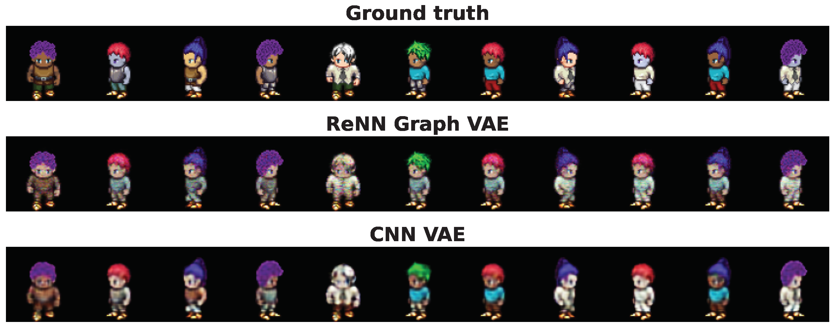
We also evaluated the performance of the model on the sprite benchmark dataset, after transforming the image data into graphs. Although it can not be directly compared with more sophisticated and task specific algorithms for image synthesis, our model has the ability to generate good quality images, create disentangled representations of features, and interpolate through samples as well as a standard CNN VAE. Finally, we performed an ablation study on pooling. The results show how, on our task on large regular graphs, using the ReNN-Pool is more efficient and leads to better performances versus using a state-of-the-art technique, such as Top-k Pool.
Finally, we believe that ReNN-Pool represents a simple, lightweight and efficient solution to pool regular graphs. It requires no computation during either the training or inference of models because node masks and adjacency matrices can be computed and stored early on. Thus, it is directly scalable to graphs of any size, contrarily to state-of-the-art pooling techniques. Moreover, the definition of a symmetrical un-pooling technique enables the construction of graph decoding modules, which can take advantage of graph convolutional layers. The current limitation of our pooling is that it has been only tested on regular graphs. However, a test on irregular graphs is among our future research directions. Although ReNN-Pool is not directly usable on all types of graphs, such as fully or highly connected ones, we believe that it could also be an efficient solution for irregular graphs with small to medium-sized node neighbourhoods. We also plan to test our method on graph U-Net architectures, where the symmetry between encoding and decoding is needed.

Author Contributions

Conceptualization, L.A., B.C., A.C., S.G. and C.M.T.; methodology, L.A., B.C., A.C., S.G. and C.M.T.; software, L.A.; validation, L.A. and A.C.; formal analysis, L.A.; investigation, L.A. and A.C.; resources, B.C., S.G. and C.M.T.; data curation, L.A. and C.M.T.; writing—original draft preparation, L.A.; writing—review and editing, L.A., A.C. and S.G.; visualization, L.A.; supervision, S.G. and C.M.T. All authors have read and agreed to the published version of the manuscript.

Funding

This research received no external funding.

Data Availability Statement

The Sprite dataset is publicly available in https://lpc.opengameart.org/, (accessed on 17 November 2022); the Energy deposition datasets and the code used for this study are available on request by contacting the authors.

Conflicts of Interest

The authors declare no conflict of interest. The funders had no role in the design of the study; in the collection, analyses, or interpretation of data; in the writing of the manuscript; or in the decision to publish the results.

Abbreviations and Symbols

The following abbreviations and symbols are used in this manuscript:
DLDeep Learning
CNNConvolutional Neural Network
GANGenerative Adversarial Networks
VAEVariational AutoEncoder
RTRadiotherapy
GNNGraph Neural Networks
GCNGraph Convolutional layers
GAEGraph AutoEncoders
VGAEVariational Graph AutoEncoders
ReNN-PoolRecursive Nearest Neighbour Pooling
ELBOEvidence Lower Bound
( z , θ , r ) Cylindrical coordinate system
X = { x i } i = 1 N Node feature vector
A = { A i , j } i , j = 1 N Adjacency matrix
MReNN-Pool masking vector
NNumber of nodes in the graph
N ( i ) Number of neighbours of node i
e i j Weight of the edge between node i and j
W k Generic weight of the Neural network
ZLatent space variable
δ δ -index

Appendix A. Full Model Description

In the following Tables, we report a detailed list of the layers that compose the models we used to run the experiments described in Section 3. Next to the name of each layer, we report the number of parameters in it and the number of nodes and edges in the graphs after the layer execution. In particular, in Table A1, we describe the model used on the Water + Slab dataset. For the Water dataset, we used the same architecture except for the last two linear layers of the encoder and the first one of the decoder, whose output (input) number of channels was set to 1, instead of 2, in accordance with the latent space dimensionality.
In Table A2, the version of the Re-NN Graph VAE used for the Sprite dataset is described. The linear layers between the pooling (un-pooling) operations and the graph convolutions are responsible for learning the edge features which enter in the computation of the GraphConv marked with e i j .
Table A1. ReNN Graph VAE used for the Water + Slab dataset. For the Water dataset, the same architecture was used but the parameter marked with an asterisk was changed to 1, in accordance with the latent space dimensionality.
LayersParametersN NodesN Edges
Graph EncoderGraphConv (1, 16, ‘mean’)4821,952128,576
ReNN-Pool-10,976188,216
GraphConv (16, 32, ‘mean’)105610,976188,216
ReNN-Pool-147021,952
GraphConv (32, 64, ‘mean’)4160147021,952
ReNN-Pool-2366206
Linear (64 × 236, 64)966,720--
Linear (64, 2*)130--
Graph DecoderLinear (2*, 64)192--
Linear (64, 64 × 236)981,760--
ReNN-Unpool-147021,952
GraphConv (64, 32, ‘mean’)4128147021,952
ReNN-Unpool-10,976188,216
GraphConv (32, 16, ‘mean’)104010,976188,216
ReNN-Unpool-21,952128,576
GraphConv (16, 1, ‘mean’)3321,952128,576
Table A2. ReNN Graph VAE for sprite dataset.
LayersParametersN NodesN Edges
Graph EncoderGraphConv (3, 16, ‘mean’)112409616,128
ReNN-Pool-204815,874
Linear (1, 15,874)31,748--
GraphConv (16, 32, ‘mean’, e i j )1056204815,874
ReNN-Pool-5283906
Linear (1, 3906)7812--
GraphConv (32, 64, ‘mean’, e i j )41605283906
ReNN-Pool-136930
Linear (64 × 136, 64)557,120--
Linear (64, 5)325--
Linear (64, 5)325--
Graph DecoderLinear (5, 64)384--
Linear (64, 64 × 136)565,760--
ReNN-Unpool-5283906
Linear (1, 3906)7812--
GraphConv (64, 32, ‘mean’, e i j )41285283906
ReNN-Unpool-204815,874
Linear (1, 15,874)31,748--
GraphConv (32, 16, ‘mean’, e i j )1040204815,874
ReNN-Unpool-409616,128
GraphConv (16, 3, ‘mean’)99409616,128

Appendix B. Variational AutoEncoder

A Variational AutoEncoder is a generative Deep Learning model first proposed by Kingma and Welling [2]. It is a special AutoEncoder based on the variational Bayes inference, whose goal is to learn the distribution of the training data and to be able to sample new datapoints from it. The underlying hypothesis is that datapoints { x } are the results of a generative process controlled by a variable z that lives in a low dimensional space, called latent space, and their distribution is thus:
p ( x ) = p ( x | z ) p ( z ) d z ,
where the prior p ( z ) is often considered Gaussian. The model is made up of two networks: the encoder and the decoder. The encoder q ψ ( z | x ) maps the input data to a distribution in the latent space. Thanks to the reparemeterisation trick, a point from such a distribution is sampled in a fully differentiable way and processed by the decoder p ψ ( x | z ) to retrieve the original data. The model is trained maximising the evidenced lower bound (ELBO) of the data likelihood:
{ ψ , ϕ } = a r g m a x ψ , ϕ E x q ψ ( · | x ) l o g p ϕ ( x | z ) D K L ( q ψ ( z | x ) | p ( z ) )
After training, new datapoints x can be generated sampling z in the latent space and passing it to the decoder. Starting from a standard VAE, it is also possible to slightly modify the loss function by adding a scalar hyperparameter β > 1 :
{ ψ , ϕ } = a r g m a x ψ , ϕ E x q ψ ( · | x ) l o g p ϕ ( x | z ) β D K L ( q ψ ( z | x ) | p ( z ) ) .
The model with such a modification is known as β -VAE [35] and is recognised to promote a better disentangling of features’ embedding in the latent space.

Appendix C. ReNN Graph VAE vs. CNN VAE

We performed a quantitative comparison between our ReNN Graph VAE and a standard 2D CNN VAE on the Sprite benchmark dataset. The CNN comprise 2D convolutional layers and mean pooling in the encoder and 2D transpose convolutions and upsampling in the decoder. A full description of the model is given in Table A3. The model was trained for 50 epochs with a batch size of 50, setting the latent space to have 5 dimensions. For the weight update, we used the Adam optimiser with an initial learning rate of 0.005 and an exponential scheduler with λ = 0.95. In order to obtain a disentangled representation for the hair style in the latent space, we had to set the β parameter to 4.
To quantitatively evaluate the performance of our model on this dataset, we considered the Structure Similarity Index Measure (SSIM). It is a perception-based measure that considers image degradation as the perceived change in structural information. While pixel-per-pixel reconstruction metrics, such as as MSE or the previously used δ -index, estimate absolute errors, the structural information considers the strong inter-dependencies between spatially close pixels that carry important information about the image as a whole. Both CNN VAE and ReNN Graph VAE reached an average SSIM on the test set of 0.90 .
In Figure A1, we also report a comparison between some ground truth, ReNN Graph VAE reconstructed sprites and CNN VAE reconstructed sprites from the test set. Both VAEs work well, but it is possible to spot some differences. CNN VAE reconstructed images are slightly blurrier that the originals, while the ReNN Graph VAE has slightly less bright colours.
Figure A1. Ground truth vs. reconstructed sprites. Comparison between sprites from the test set with their reconstructed counterpart by ReNN Graph VAE and a standard CNN VAE.
Algorithms 16 00143 g0a1
Table A3. Two-dimensional CNN VAE for sprite dataset.
LayersParameters
Graph EncoderConv2d (3, 16, kernel_size = (3, 3, 3))448
AvgPool2d (kernel_size = 2, stride = 2)-
Conv2d (16, 32, kernel_size = (3, 3, 3))4640
AvgPool2d (kernel_size = 2, stride = 1)-
Conv2d (32, 64, kernel_size = (3, 3, 3))18,496
AvgPool2d (kernel_size = 2, stride = 2)-
Linear (64 × 169, 64)692,288
Linear (64, 5)325
Linear (64, 5)325
Graph DecoderLinear (5, 64)384
Linear (64, 64 × 169)703,040
Upsample (size = (26, 26), mode = ‘bilinear’)-
ConvTranspose2d (64, 32, kernel_size = (3, 3, 3))18,464
Upsample (size = (29, 29), mode = ‘bilinear’)-
ConvTranspose2d (32, 16, kernel_size = (3, 3, 3))4624
Upsample (size = (62, 62), mode = ‘bilinear’)-
ConvTranspose2d (16, 3, kernel_size = (3, 3, 3))435

References

  1. Goodfellow, I.J.; Pouget-Abadie, J.; Mirza, M.; Xu, B.; Warde-Farley, D.; Ozair, S.; Courville, A.; Bengio, Y. Generative Adversarial Networks. arXiv 2014, arXiv:1406.2661. [Google Scholar] [CrossRef]
  2. Kingma, D.P.; Welling, M. Auto-Encoding Variational Bayes. arXiv 2014, arXiv:1312.6114. [Google Scholar]
  3. Rezende, D.; Mohamed, S. Variational Inference with Normalizing Flows. In Proceedings of the Machine Learning Research (PMLR), Proceedings of the 32nd International Conference on Machine Learning, Lille, France, 6–11 July 2015; Volume 37, pp. 1530–1538. [Google Scholar]
  4. Bond-Taylor, S.; Leach, A.; Long, Y.; Willcocks, C.G. Deep Generative Modelling: A Comparative Review of VAEs, GANs, Normalizing Flows, Energy-Based and Autoregressive Models. IEEE Trans. Pattern Anal. Mach. Intell. 2022, 44, 7327–7347. [Google Scholar] [CrossRef]
  5. Mentzel, F.; Kröninger, K.; Lerch, M.; Nackenhorst, O.; Paino, J.; Rosenfeld, A.; Saraswati, A.; Tsoi, A.C.; Weingarten, J.; Hagenbuchner, M.; et al. Fast and accurate dose predictions for novel radiotherapy treatments in heterogeneous phantoms using conditional 3D-UNet generative adversarial networks. Med. Phys. 2022, 49, 3389–3404. [Google Scholar] [CrossRef]
  6. Zhang, X.; Hu, Z.; Zhang, G.; Zhuang, Y.; Wang, Y.; Peng, H. Dose calculation in proton therapy using a discovery cross-domain generative adversarial network (DiscoGAN). Med. Phys. 2021, 48, 2646–2660. [Google Scholar] [CrossRef] [PubMed]
  7. Mendonça, R.V.; Silva, J.C.; Rosa, R.L.; Saadi, M.; Rodriguez, D.Z.; Farouk, A. A lightweight intelligent intrusion detection system for industrial internet of things using deep learning algorithms. Expert Syst. 2022, 39, e12917. [Google Scholar] [CrossRef]
  8. Beniczky, S.; Karoly, P.; Nurse, E.; Ryvlin, P.; Cook, M. Machine learning and wearable devices of the future. Epilepsia 2021, 62, S116–S124. [Google Scholar] [CrossRef]
  9. Khan, N.; Ullah, A.; Haq, I.U.; Menon, V.G.; Baik, S.W. SD-Net: Understanding overcrowded scenes in real-time via an efficient dilated convolutional neural network. J. Real-Time Image Process. 2021, 18, 1729–1743. [Google Scholar] [CrossRef]
  10. Francescato, S.; Giagu, S.; Riti, F.; Russo, G.; Sabetta, L.; Tortonesi, F. Model compression and simplification pipelines for fast deep neural network inference in FPGAs in HEP. Eur. Phys. J. C 2021, 81, 969. [Google Scholar] [CrossRef]
  11. Morris, C.; Ritzert, M.; Fey, M.; Hamilton, W.L.; Lenssen, J.E.; Rattan, G.; Grohe, M. Weisfeiler and Leman Go Neural: Higher-order Graph Neural Networks. arXiv 2021, arXiv:1810.02244. [Google Scholar] [CrossRef] [Green Version]
  12. Kipf, T.N.; Welling, M. Semi-Supervised Classification with Graph Convolutional Networks. arXiv 2017, arXiv:1609.02907. [Google Scholar]
  13. Defferrard, M.; Bresson, X.; Vandergheynst, P. Convolutional Neural Networks on Graphs with Fast Localized Spectral Filtering. arXiv 2017, arXiv:1606.09375. [Google Scholar]
  14. Veličković, P.; Cucurull, G.; Casanova, A.; Romero, A.; Liò, P.; Bengio, Y. Graph Attention Networks. arXiv 2018, arXiv:1710.10903. [Google Scholar]
  15. Zhu, Y.; Du, Y.; Wang, Y.; Xu, Y.; Zhang, J.; Liu, Q.; Wu, S. A Survey on Deep Graph Generation: Methods and Applications. arXiv 2022, arXiv:2203.06714. [Google Scholar]
  16. Kipf, T.N.; Welling, M. Variational Graph Auto-Encoders. arXiv 2016, arXiv:1611.07308. [Google Scholar]
  17. Dhillon, I.S.; Guan, Y.; Kulis, B. Weighted Graph Cuts without Eigenvectors A Multilevel Approach. IEEE Trans. Pattern Anal. Mach. Intell. 2007, 29, 1944–1957. [Google Scholar] [CrossRef]
  18. Zhang, M.; Cui, Z.; Neumann, M.; Chen, Y. An End-to-End Deep Learning Architecture for Graph Classification. In Proceedings of the AAAI Conference on Artificial Intelligence, New Orleans, LA, USA, 2–7 February 2018; Volume 32. [Google Scholar] [CrossRef]
  19. Bianchi, F.M.; Grattarola, D.; Livi, L.; Alippi, C. Hierarchical Representation Learning in Graph Neural Networks with Node Decimation Pooling. IEEE Trans. Neural Netw. Learn. Syst. 2022, 33, 2195–2207. [Google Scholar] [CrossRef]
  20. Bravo-Hermsdorff, G.; Gunderson, L.M. A Unifying Framework for Spectrum-Preserving Graph Sparsification and Coarsening. arXiv 2020, arXiv:1902.09702. [Google Scholar]
  21. Ying, R.; You, J.; Morris, C.; Ren, X.; Hamilton, W.L.; Leskovec, J. Hierarchical Graph Representation Learning with Differentiable Pooling. arXiv 2019, arXiv:1806.08804. [Google Scholar]
  22. Gao, H.; Ji, S. Graph U-Nets. arXiv 2019, arXiv:1905.05178. [Google Scholar] [CrossRef]
  23. Ranjan, E.; Sanyal, S.; Talukdar, P. Asap: Adaptive structure aware pooling for learning hierarchical graph representations. In Proceedings of the AAAI Conference on Artificial Intelligence, New York, NY, USA, 7–12 February 2020; Volume 34, pp. 5470–5477. [Google Scholar]
  24. Guo, Y.; Zou, D.; Lerman, G. An Unpooling Layer for Graph Generation. arXiv 2022, arXiv:2206.01874. [Google Scholar]
  25. Liu, Q.; Allamanis, M.; Brockschmidt, M.; Gaunt, A.L. Constrained Graph Variational Autoencoders for Molecule Design. arXiv 2019, arXiv:1805.09076. [Google Scholar]
  26. Bresson, X.; Laurent, T. A Two-Step Graph Convolutional Decoder for Molecule Generation. arXiv 2019, arXiv:1906.03412. [Google Scholar]
  27. Guo, X.; Zhao, L.; Qin, Z.; Wu, L.; Shehu, A.; Ye, Y. Interpretable Deep Graph Generation with Node-Edge Co-Disentanglement. In Proceedings of the 26th ACM SIGKDD International Conference on Knowledge Discovery & Data Mining, Virtual, 6–10 July 2020; pp. 1697–1707. [Google Scholar] [CrossRef]
  28. Assouel, R.; Ahmed, M.; Segler, M.H.; Saffari, A.; Bengio, Y. DEFactor: Differentiable Edge Factorization-based Probabilistic Graph Generation. arXiv 2018, arXiv:1811.09766. [Google Scholar]
  29. Du, Y.; Guo, X.; Cao, H.; Ye, Y.; Zhao, L. Disentangled Spatiotemporal Graph Generative Models. In Proceedings of the AAAI Conference on Artificial Intelligence, Virtual, 22 February–1 March 2022; Volume 36, pp. 6541–6549. [Google Scholar] [CrossRef]
  30. Shelhamer, E.; Long, J.; Darrell, T. Fully Convolutional Networks for Semantic Segmentation. IEEE Trans. Pattern Anal. Mach. Intell. 2017, 39, 640–651. [Google Scholar] [CrossRef]
  31. Lin, B.; Gao, F.; Yang, Y.; Wu, D.; Zhang, Y.; Feng, G.; Dai, T.; Du, X. FLASH Radiotherapy: History and Future. Front. Oncol. 2021, 11. [Google Scholar] [CrossRef]
  32. Agostinelli, S.; Allison, J.; Amako, K.; Apostolakis, J.; Araujo, H.; Arce, P.; Asai, M.; Axen, D.; Banerjee, S.; Barrand, G.; et al. Geant4—A simulation toolkit. Nucl. Instruments Methods Phys. Res. Sect. A Accel. Spectrometers Detect. Assoc. Equip. 2003, 506, 250–303. [Google Scholar] [CrossRef] [Green Version]
  33. Li, Y.; Mandt, S. Disentangled Sequential Autoencoder. arXiv 2018, arXiv:1803.02991. [Google Scholar]
  34. Low, D.A.; Harms, W.B.; Mutic, S.; Purdy, J.A. A technique for the quantitative evaluation of dose distributions. Med. Phys. 1998, 25, 656–661. [Google Scholar] [CrossRef]
  35. Higgins, I.; Matthey, L.; Pal, A.; Burgess, C.; Glorot, X.; Botvinick, M.; Mohamed, S.; Lerchner, A. beta-VAE: Learning Basic Visual Concepts with a Constrained Variational Framework. In Proceedings of the International Conference on Learning Representations, Toulon, France, 24–26 April 2017. [Google Scholar]
Figure 1. Pooling. The ReNN-Pool operation consists of two steps: masking and rewiring. In the first step, recursively on the whole graph, a node is selected and all its nearest neighbours are dropped. In the second step, nodes are linked to the ones that were their 2nd order neighbours.
Algorithms 16 00143 g001
Figure 2. Un-Pooling. The Un-Pool operation consists in embedding the nodes of a pooled graph in their initial position in the bigger original graph structure. All other restored nodes are initialized to 0.
Algorithms 16 00143 g002
Figure 3. Full scheme. Schematic representation of our Re-NN Graph VAE with two encoding blocks and two decoding blocks. Each block is made up of a graph convolution and a pooling (un-pooling) operation. In the lower part of the picture, the VAE sampling and the encoding (decoding) linear layers are represented.
Algorithms 16 00143 g003
Figure 4. Dataset and ReNN-Pool. From the left, the panels show the representation of a typical example from the energy deposition datasets and two pooled representations of the same example. The nodes in light grey have null features, while all others show an energy distribution within the considered range.
Algorithms 16 00143 g004
Figure 5. Energy profiles reconstruction. Distribution of energy deposition along z and r axes from the test sets of the Water dataset (a) and the Water + Slab dataset (b). The blue lines correspond to the Monte Carlo simulated data, while the orange lines refer to the reconstructed data from our Network.
Algorithms 16 00143 g005aAlgorithms 16 00143 g005b
Figure 6. Standard deviations in MC and VAE. Comparison of standard deviation over mean of the energy profile along the z axis between Monte Carlo simulations and VAE reconstruction in the Water + Slab setting. Values are estimated for 100 MC runs with fixed parameters and 100 VAE execution with the same example as input. Results demonstrate how VAE’s largest errors are in regions where energy deposition fluctuation, and so Monte Carlo’s ones, are not negligible.
Algorithms 16 00143 g006
Figure 7. Results on sprite dataset. (a) Comparison between input sprite images (first row) and reconstructed ones (second row). (b) Images generated fixing all the latent variables’ dimensions but one, which is varied. Generated sprites have fixed attributes but a continuously varying hair style.
Algorithms 16 00143 g007
Table 1. Results on energy deposition reconstruction. We report mean relative errors on energy profiles and total energy along with the mean 3% δ -index passing rate. Uncertainties are computed as standard deviations. Values are computed on test sets.
Datasetz Profile Errorr Profile ErrorTotal Energy Error δ < 3%
Water5.8 ± 3.4%2.6 ± 1.6%2.2 ± 1.6%99.3 ± 0.1%
Water + Slab6.9 ± 3.4%3.0 ± 1.2%2.2 ± 1.6%98.6 ± 0.3%
Table 2. Results of ablation study on pooling. Comparison of the results on the test set of the Water + Slab dataset using different pooling and un-pooling techniques. Mean relative errors on energy profiles and total energy along with the mean 3% δ -index passing rate on test sets are reported.
Poolingz Profile Errorr Profile ErrorTotal Energy Error δ < 3 %
ReNN-Pool6.9 ± 3.4%3.0 ± 1.2%2.2 ± 1.6%98.6 ± 0.3%
ReNN Mean Pool6.4 ± 3.0%2.8 ± 1.1%2.0 ± 1.4%98.6 ± 0.3%
ReNN Max Pool22.6 ± 9.9%5.0 ± 1.8%3.2 ± 2.3%97.5 ± 0.7%
Random Pool172.6 ± 21.7%52.2 ± 3.7%2.0 ± 1.5%92.4 ± 0.4%
Top-k Pool51.7 ± 3.4%75.1 ± 9.1%4.0 ± 2.6%79.9 ± 1.3%
Disclaimer/Publisher’s Note: The statements, opinions and data contained in all publications are solely those of the individual author(s) and contributor(s) and not of MDPI and/or the editor(s). MDPI and/or the editor(s) disclaim responsibility for any injury to people or property resulting from any ideas, methods, instructions or products referred to in the content.

