1. Introduction
The main task of layout recognition is to generate bounding boxes or polygons for the text elements of a page together with their reading order as a prerequisite for the subsequent optical character recognition (OCR) step in an optical document recognition (ODR) pipeline. While this task is easy for simple text pages, it can become quite complicated for historical documents, which contain features such as multiple column layouts, marginalia, headers, footers, including page numbers or catchwords, images, or dropped capitals (e.g., decorated initials), which require being able to recognize them. Since visual elements are not transcribed, they only need to be separated from the text. Errors in layout recognition have disastrous consequences for the OCR step. Therefore, a manual layout correction step is usually necessary in practical ODR pipelines. Our goal was to avoid this step or—for high-quality transcriptions—to integrate it with the OCR correction step.
Public datasets for the layout recognition of historic documents such as the OCR-D collection include a great variety of pages with different layouts. It is still a challenge to achieve a high precision and recall in recognizing all the features with a generic approach. However, in practical projects, it is possible to specify the layout features used in a particular print (book) to be transcribed and to use this knowledge to improve the quality of the layout recognition. Different historical books have different layouts with a limited amount of special features and a regular structure, the knowledge of which can greatly simplify the layout recognition task.
In
Section 2, an overview of the related work, comprised of quite different approaches, is presented. In the next section, publicly available data sources are presented, and our own datasets with several pages taken from different historical books representing typical practical tasks are described. In
Section 4, the architecture and training conditions of the machine learning models, as well as the postprocessing methods used are described in detail.
Section 5 explains our proposed evaluation metrics.
Section 6.1 describes the various experiments performed using different methods and on different datasets.
Section 7 presents the results.
Section 8 discusses the strengths and weaknesses of the results, together with an analysis of the errors made, and
Section 9 presents the summary and the outlook for future work.
2. Related Work
Layout analysis is an important first step in the digitization and processing of document images. In general, the layout analysis task can be described as detecting regions of different semantic types in the document image [
1]. One important aspect to consider for this task is the detail level at which the page layout should be analyzed. While there are many approaches focusing only on text, non-text, and background segmentation, recent approaches tend to classify elements on the page into increasingly more refined categories. As an example, for the common PubLayNet dataset [
2], the goal is to detect the main text regions, titles, figures, tables, and lists. Recently, due to the rise of increasingly capable NLP models, the tasks in layout analysis can also involve the classification of the semantic roles of the text inside the various regions, as described in [
3]. Here, the authors compared textual to hybrid approaches such as LayoutLM and visual approaches such as YoLoV5 [
4], to distinguish the text roles such as primary text, commentaries, translations, and critical apparatuses in datasets from the 19th Century.
As our paper mainly focused on the visual aspect of layout recognition, we present primarily visual approaches for this task in the following. This is especially of interest regarding the fact that many more detailed approaches often require a prior step, in which text elements have already been extracted and transcribed.
Although the task of layout recognition can be approached using a single step using modern neural networks, as for example described in [
5], many related works still focus on improving individual aspects of the pipeline, such as text or illustration detection in historical documents or table recognition in modern documents.
Three main types of approaches to this problem can be identified, which differ in their roles in complete document processing pipelines, as well as their produced outputs. The first category comprises pixel-level segmentation approaches. Such methods take a document image as the input and assign a class label to each individual pixel in the image. The labels can range from just a text/non-text distinction to individual class labels for different types of text elements such as headings, footers, titles, the main text, etc. Clearly, these methods are just a first step in the layout analysis as, for the subsequent OCR, individual regions or text lines have to be extracted from the output in a postprocessing step, as such annotations are a requirement for the subsequent OCR and further document processing [
6]. This can be challenging if the output of the segmentation is not perfectly accurate, which could lead to the reduced performance of the text recognition system. The second category comprises text detection approaches, which focus on the localization of textual elements, such as printed lines, or handwritten notes, or even handwritten artifacts on printed pages. It is important to note that these approaches differ from the segmentation category, as their goal is not only to detect the location of text elements, but also to determine the individual instances of text objects, such as individual lines in the document image. These methods have the advantage of the detected textual elements being able to be directly fed into the OCR. In addition, the document’s visual layout can easily be reconstructed from the detection, as the locations of the text elements are also detected in this process. The last category of methods can be described as generic instance-level segmentation approaches. Similar to the task in [
1], the goal of these methods is to extract the region instances of layout elements such as text lines, text regions, title regions, dropped capital regions, as well as non-text instances, such as illustrations, figures, or separators. This category can be seen as a combination of the two prior categories, as these approaches deliver classified regions, which can be directly fed into OCR engines for further processing. In addition to that, the document’s visual layout can be reconstructed after the OCR using the region information.
In the following, we present some approaches for each category. For the last category, we provide a detailed analysis, as these are most comparable to our method for layout recognition.
2.1. Pixel-Level Segmentation
As previously mentioned, since OCR systems require regions or text lines as the input, further postprocessing has to be applied to use these systems in a document processing pipeline. Although there exist methods to identify individual text lines in the output of such labeled document images, it is not trivial to generate a full layout segmentation from the labeled output. Especially, when it comes to more complex multi-column layouts, the page segmentation task might not provide sufficient information to distinguish multi-column from single-column layouts, especially, when two columns are close together. Furthermore, as these methods do not detect individual lines, it might not be trivial to reconstruct a reading order from the pixel-labeled segmentation.
CNN-based methods, such as [
7,
8], rely on the classification of smaller features, such as superpixels or connected components, to build a segmented image.
Furthermore, fully convolutional neural networks such as U-Nets [
9] have shown promising results on the page segmentation task. Wick et al. [
10] used an FCN to detect page regions of different types in historical documents.
Monnier et al. [
11] used a U-Net with a modified ResNet encoder to segment historical documents. For training, their approach focused mostly on their training dataset, which consisted of synthetically generated document images. In addition, the method can be applied to detect baselines in historic documents, as explained in further detail in the next section.
Oliveira et al. [
12] used a U-Net with a ResNet-50 encoder to perform three different tasks for document layout recognition: recognizing text lines by detecting their baselines, segmenting the image by class, detecting boxes for ornaments, and recognizing the main page’s area.
Boillet et al. [
13] presented a fully convolutional network with a U shape using dilated convolutional layers to label the text lines.
2.2. Text Line Detection
The goal of text line detection is to extract individual instances of text elements or lines from the document images. This task can be approached from different angles, e.g., as a pixel-labeling task with additional postprocessing or as an object detection task featuring deep neural networks such as Mask-RCNN.
In general, the use of deep neural network techniques has reported outstanding results in many areas related to computer vision, including text line recognition. Grüning et al. treated this problem as a segmentation task [
14]. Their pipeline used a spatial-attention-based network architecture to achieve a pixel-level segmentation of the image containing the baselines of the text lines. Afterward, they applied a complex postprocessing algorithm to generate text lines from the pixel-level segmentation. In [
15], the baseline detection was extended by introducing baseline primitives and applying a relation network to further improve the results.
Alternatively, morphological and visual features can be utilized to detect text lines.
Cohen et al. [
16] present a non-ML approach using a connected component analysis and significant postprocessing of the detected contours to recognize text lines in handwritten and printed historical documents. Barakat et al. [
17] presented a method utilizing an FCN to detect text elements in a document image. In addition, they utilized a connected-component-based postprocessing to merge text lines, based on the output of the FCN.
Alternatively, the challenge can be approached as an object detection task. Droby et al. [
18] used a Mask-RCNN [
19] to detect the text line instances in historical documents. They divided the page into patches and, afterward, used a postprocessing algorithm, which combined the output. Afterwards, the text lines were extracted.
Bluche [
20] proposed a segmentation-free hand writing recognition system based on multi-dimensional long short-term memory recurrent neural networks. The method requires a rough layout analysis in advance, as it was applied to paragraph images. A separate line segmentation step was then no longer necessary, because this was implicitly performed within the network, and the network then directly provided an OCR output.
Most-commonly used OCR systems, such as [
21], require images for individual text lines. Therefore, it is either relevant for further processing of the document images to perform postprocessing on a segmentation or to detect text lines directly in the images. Baseline methods such as [
14] deliver good results, but need additional postprocessing steps to generate the required polygons describing individual lines from the baselines.
2.3. Instance-Level Segmentation for Page Layout Analysis
In addition to the previously presented methods, layout recognition can also be seen as an object detection task, where the goal is to identify semantically different regions in the image and distinguish separate instances. In contrast to labeling the image on a per-pixel level, object detection provides output bounding boxes or even masks for individual instances of detected regions in the image [
19]. This is advantageous compared to pure segmentation, as, e.g., in multi-column layouts, single columns can be detected as individual instances. In contrast to pixel-level metrics such as the mIoU or accuracy for the page segmentation task, the metrics used for the object detection task, such as the mAP or the precision/recall measures on individual instances, take the instance segmentation into account.
Clérice et al. [
22] used YoloV5 [
4] to detect twelve different page layout zones in historical documents. Afterwards, the results were injected into Kraken [
23] to generate text lines and the OCR output. Likewise, Büttner et al. [
24] applied a YoloV5 network to detect graphical elements, such as initials, decorations, printer’s marks, or content illustrations, in different historical documents.
The authors of [
5] presented a method based on instance-level segmentation based on a modified Mask-RCNN architecture to detect different layout elements in popular datasets such as PubLayNet, containing more modern document images, or the HJ dataset, containing historical Japanese document images.
A different approach was taken by [
25], who presented a Transformer-based model for instance-level segmentation. Their model consisted of a feature extracting feature pyramid network (FPN), which then was fed into a Transformer. Then, the features with global context as the output from the Transformer were combined with the local FPN features to form the final segmentation and instance segmentation outputs. An approach utilizing different input representations for modern documents was presented by Zhang et al. [
26]. They used the page’s input in conjunction with CharGrid and SentGrid representations of the document to build a layout recognition model using a separate visual and semantic part consisting of convolutional neural networks, which were then combined in a multiscale adaptive aggregation module. The outputs of this module were fed into a graph neural network, which postprocessed the resulting region proposals to produce the final instance-level segmentation of the document.
A rule-based approach for instance-level page segmentation was presented by [
27]. In this system, a set of handcrafted rules is applied to classify text lines and text regions into different semantic classes such as title, first line, header, text, or other on a custom French newspaper dataset. In addition, the authors utilized the RIPPER method to automatically induce the rules for the classification from a training dataset. However, it has to be noted that this method requires text regions and the corresponding OCR as the input. This is also a key difference from our proposed method, as our rule-based system does not rely on annotation regions and OCR, but instead, only on the output of a baseline detector with additional postprocessing.
The comparison of different layout segmentation approaches is difficult, as individual methods are usually evaluated on different datasets. Although for modern document layouts, datasets such as PubLayNet [
2] exist and provide a common ground for comparison, there are only a few commonly used datasets for historical documents, such as the IlluHisDoc dataset [
11] for illustration detection or the DivaHisDB dataset [
28] for the segmentation of different text categories. In addition, there exist multiple metrics for layout recognition, as different outputs require different metrics. For example, the pixelwise segmentation task could be evaluated using the foreground pixel accuracy [
10] or the mean IoU of individual classes, and layout recognition methods based on object detection methods use the AP measure [
29]. For our approach, we were not able to calculate the AP as defined in [
29], as our method does not produce confidence values for the predicted elements. Furthermore, metrics such as the mAP or mIoU are not easily interpretable.
In
Table 1, several previously mentioned layout analysis methods are presented and their most-relevant results are compared. As can be seen from the table, especially for modern document types, layout recognition approaches such as [
25] provide good results.
The approach of Zhang et al. [
26] also showed a high AP of 95.69%. However, it has to be noted that the input for this method requires the annotation of individual characters’ bounding boxes and the corresponding character embedding as an input and is thus mostly suitable for the analysis of documents that are either available in digital form, such as PDF, or have been previously transcribed by another OCR system.
For historical documents, however, the results of recent methods have not been promising. For the illustration segmentation task, References [
11,
24] showed promising results for the in-domain experiment. When looking at the out-of-domain case, the results were significantly lower, suggesting that commonly used networks such as U-Nets and YoloV5 are not able to generalize well to previously unseen data for the layout recognition task.
Furthermore, the performance of object detection methods has previously been compared to the performance of commonly used open-source page segmentation and OCR systems, such as Tesseract [
30] or Kraken [
23]. In [
22], the comparison to Kraken suggests that their object-detection approach significantly outperformed the region-based segmentation used in the Kraken engine. In [
11], the authors compared their baseline detection to the open-source tool Tesseract4 and showed that training their baseline detection method on purely synthetically generated data improved significantly over the performance of Tesseract4 when evaluated on the cBAD17 and cBAD19 datasets.
Nevertheless, especially for historical documents, where text elements have to be categorized by their context, this work also suggests the limitations of pure object detectors such as YoloV5 [
22] for historical layout analysis, as the AP of
was significantly lower than the current state-of-the-art for modern documents, which have achieved an mAP as high as
[
25]. Although, it has to be noted that, for the historical documents, the task is more challenging as nearly three-times as many classes have to be distinguished.
Table 1.
Comparison of different layout analysis methods. The training and evaluation datasets, as well as the output of the methods are given in the figure. The evaluated layout elements, the metrics used for evaluation, as well as the results are presented. In addition, some relevant results for comparison architectures are given. Lines with dots indicate the same entry as above. 1 A preprocessed document with physical layout annotations and OCR was used as the input. 2 Character and sentence embedding maps were used as an additional input. * Values have been averaged from the original source’s results.
| Source | Year | Input
Anno-
tations | Dataset
(Training) | Dataset
(Evaluation) | Output | Detected
Layout
Elements | Method | Metric | Results |
|---|
YALTAi
[22] | 2022 | no | YALTAi-
MSS-EP | YALTAi-
MSS-EP | Regions | 12 region types | YoloV5x | mAP | 47.8% |
| | | | . | . | | . | Kraken | mAP | 69.8% |
Biswas
et al. [5] | 2021 | no | PubLayNet | PubLayNet | Regions | Text, Title, List,
Table, Figure | Custom
Network | Detection
AP | 92.0% |
| | | | . | . | . | . | . | Segmen-
tation AP | 89.3% |
| | | | . | . | . | . | Mask-RCNN | Detection
AP | 91.0% |
VSR
[26] | 2021 | yes 2 | PubLaynet | PubLayNet | Regions | Text, Title, List,
Table, Figure | Custom | AP | 95.7% |
| | | | . | . | | . | Mask RCNN | AP | 90.7% |
Büttner
et al. [24] | 2022 | no | S-VED
extended | illuHisDoc
(1280 × 1280) | Regions | Initial
Illustrations | YoloV5 | AP | 69.3% |
| | | | . | illuHisDoc
(640 × 640) | . | . | . | AP | 79.3% |
| | | | S-VED | S-VED
extended
(1280 × 1280) | . | . | . | AP | 96.2% |
| | | | SynDoc | illuhisDoc
(1280 × 1280) | . | . | . | AP | 82.6% |
dhSeg-
ment [12] | 2019 | no | DIVA-HisDB | DIVA-HisDB | Pixel Seg-
mentation | Background,
Initial, Com-
ment, Text | U-Net with
ResNet50
Encoder | IoU (avg) | 93.8% |
| | | no | Custom Or-
nament DS | Custom Or-
nament DS | Regions | Ornamnets | As above
+ Postprocesing | IoU | 87.0% |
docSeg
Tr [25] | 2022 | no | PubLayNet | PubLayNet | Regions | Text, Title,
List, Table,
Figure | Custom
Transformer
Net | Segmen-
tation AP | 89.4% |
Gutehrlé
et al. [27] | 2022 | yes 1 | Custom
French
Newspaper | Custom
French
Newspaper | Semantical-
ly Labeled
Text Line
Instances | TextLine: text | Rule-Based | F1 Text | 97.9% |
| | | | . | . | . | . | Rule-Based
(RIPPER) | F1 Text | 90.1% |
| | | | . | . | . | TextLine: Text,
Title, Firstline,
Header | Rule-Based | Macro
Avg F1 (*) | 73.9% |
| | | | . | . | . | . | Rule-Based
(RIPPER) | Macro
Avg F1 (*) | 51.5% |
| Ours | 2023 | no | cBAD,
Custom
Historical | Custom
Historical | Semantical-
ly Labeled
Text Line
Instances | Text/Non-Text | Baseline-
Detection,
Rule-Based,
Mask-RCNN
(Initials) | Macro
Avg F1
( Text/
Non-Text ) | 99.3% |
| | | | . | . | . | Text, Column, Marginalia, Header, Footer | As above + manual user settings | Macro Avg F1 (Text Elements) | 97.7% |
3. Datasets
In this section, the datasets used for the evaluation are presented. In addition, the page elements to detect are described.
3.1. Datasets Used
As mentioned above, we used five datasets for our evaluation, covering different layout styles from the 15th and 16th Centuries, instead of one combined dataset with pages from many different books with different layouts and levels of difficulty. For each page in the datasets, the layout elements were annotated manually as the ground truth (GT) on the line level, since lines are the input for the subsequent OCR step. A general difficulty is the GT annotation of the height of a line, because in some layouts, letters from two adjacent lines touch each other. We used a complex algorithm to find the best polygon for line separation, but this is difficult to evaluate against a manual GT, because it would be too time-consuming to define these polygons manually. Therefore, the GT for lines allows any “reasonable” cut between adjacent lines. A different situation exists for the length of the line polygons, since cutting one letter or even half of a letter at the beginning or end of a text line would have a negative impact on the OCR, which is taken into account by the GT and the evaluation.
The characteristics of the five datasets are as follows:
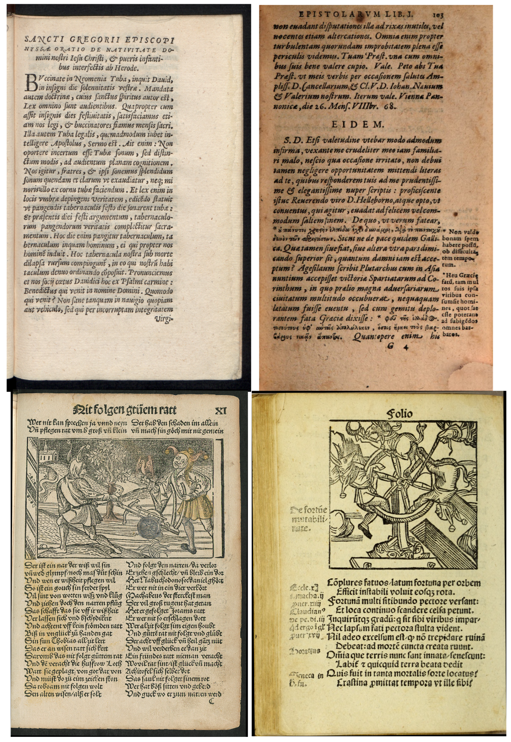
The
GW5051 dataset is a subset of a print from 1497 digitized by the
Staatsbibliothek Berlin (
https://digital.staatsbibliothek-berlin.de/werkansicht/?PPN=PPN799202126 (accessed on 10 November 2022)) and consists of 142 page images. We selected it because of its two-column layout. Different from the above datasets, it does not have a justified print, but a ragged right side. It contains many images, but no marginalia. Its top line is composed of a headline (belonging to the reading order), a page number (a header element not belonging to the reading order), and a footer.
The
GW5056 dataset is a subset of a print from 1497, made available by the
John Carter Brown Library (
https://archive.org/details/stultiferanauisn00bran/mode/2up (accessed on 10 November 2022)) and contains 150 page images. It is similar to the
GW5051 dataset, but has marginalia instead of a two-column layout and has a simpler header.
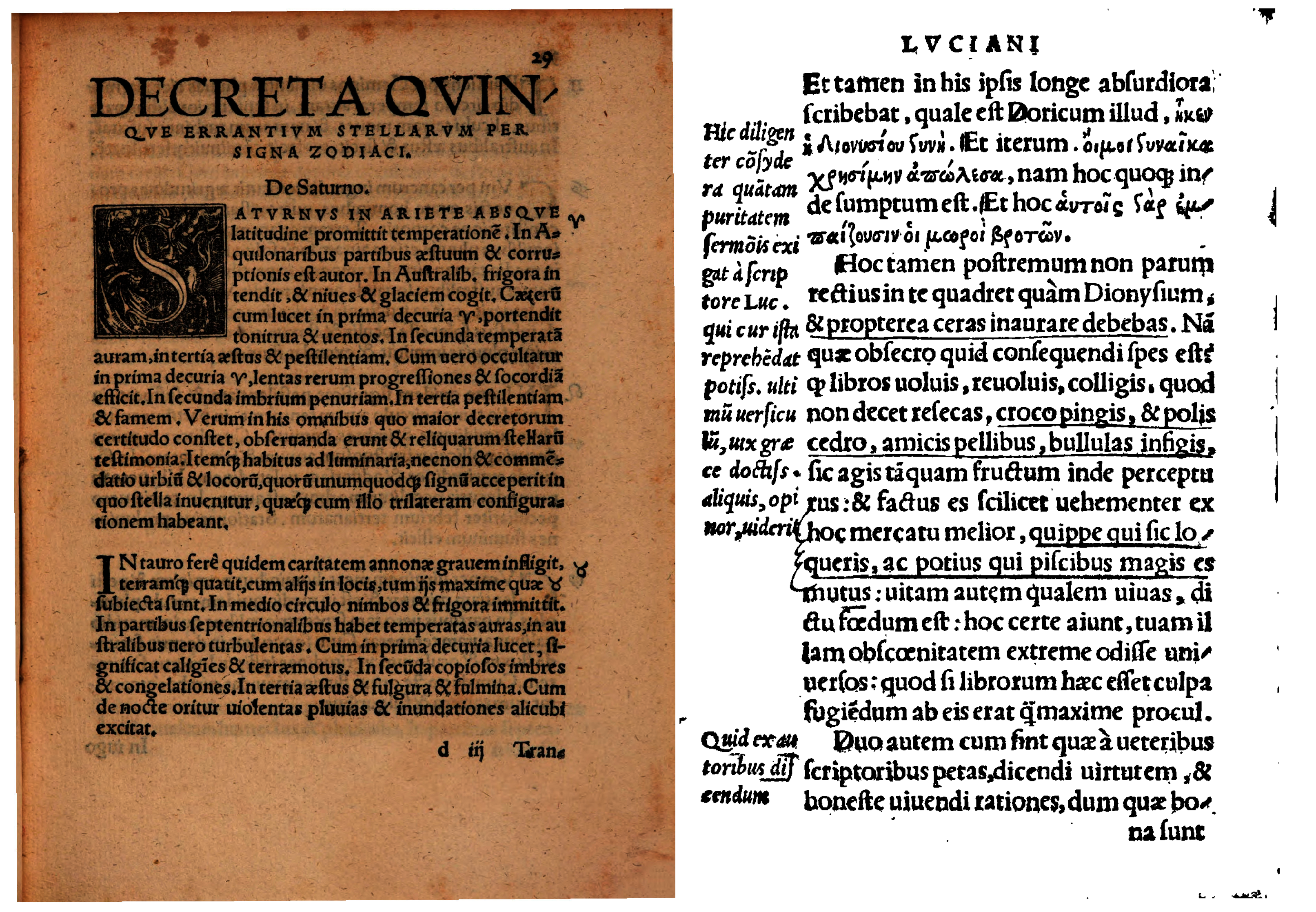
The
CamManual dataset is composed of three historical prints from 1523, 1532, and 1611 (
http://kallimachos.uni-wuerzburg.de/camerarius/index.php/Camerarius,_Astrologica_(griech.),_1532 (accessed on 10 November 2022);
http://kallimachos.uni-wuerzburg.de/camerarius/index.php/Camerarius,_Luciani_adversus_indoctum_sermo_(lat.),_1523 (accessed on 10 November 2022);
http://kallimachos.uni-wuerzburg.de/camerarius/index.php/Camerarius,_Annotatio_rerum_praecipuarum,_1611 (accessed on 10 November 2022)). It is similar to the CamMarg dataset, but contains additional manual elements such as underlines in the text and astrological symbols as marginalia and suffers from some degradation, where small parts of the text are black. We did not specify background knowledge for the manual elements; therefore, this dataset was used to evaluate the robustness of the approach.
Example pages for the first four datasets are shown in
Figure 1 and for the
CamManual dataset in
Figure 2.
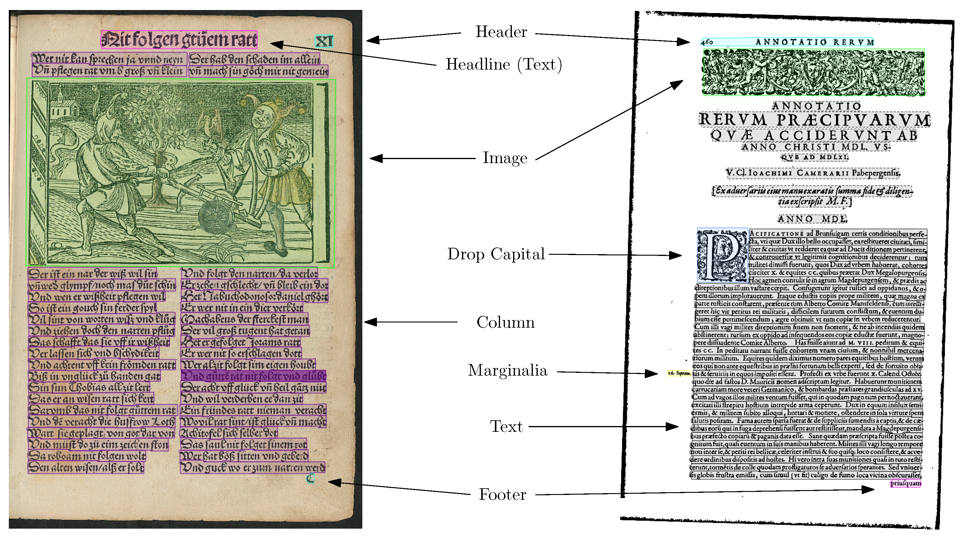
3.2. Annotated Page Elements
For the reconstruction of the reading order, the line-level layout analysis should detect all elements, which must be treated differently than concatenating lines from left to right and top to bottom. Such elements are header and footer lines and marginalia on either the left or right side, which are not part of the reading order. Furthermore, a two-column layout of the text must be recognized. Headlines do not influence the reading order. Therefore, they were treated as text, but they can be differentiated by a postprocessing step based on the font style and size and the centered layout if necessary. Images can be ignored, but a special image type must be recognized: dropped capitals look like an image in some cases, but semantically represent a letter. Therefore, we annotated the corpora with six categories.
These elements describe the main text elements that should be included in a running text representation of a historical print. In order to generate the running representation, the OCR of the text elements should be concatenated in vertical order.
As some pages contain multiple columns of text, the reading order must be adjusted. Therefore, it is important to differentiate these lines from regular text lines, as the text in columns should be read in the column-first order.
In many historical prints, marginalia are printed on the left or right of the main text lines. Such marginalia might contain additional notes, references to the original, or line numbers. They may be viewed as a correlate for modern footnotes. They do not belong to the reading order of the normal text, but should be recognized as text and attached to the corresponding text line.
On many pages, headers containing the name of the chapter or the print, as well as page numbers are included. They help maintain an overview ofthe book and should not be included in the main running text representation and the reading order. There is no differentiation between further semantic types, such as page numbers, folio number, etc., because this is best performed based on the result of the OCR step, which was not the focus of this paper.
Similar to header elements, footer elements such as catchwords or signature marks should not count as the main text and be excluded from the reading order. Similar to header elements, footer elements are not split into their different sub-categories, but are merged into a single line polygon.
Dropped capitals are usually found at the beginning of paragraphs and usually represent the first character or word of the first line of said paragraph. Dropped capitals are printed larger, often spanning multiple lines of text, which is thereby indented, and are often decorated. Therefore, even if they technically are the first letter of a text line, it is disadvantageous to include them in said line, as they significantly differ in size and visual appearance and, therefore, would constitute a challenge for the subsequent OCR.
Figure 3 shows these elements on two example pages from our used datasets.
In addition to the above-mentioned elements, historical prints might also contain images. These are also annotated in the GT and, thus, included in our evaluation, as these elements could falsely be detected as text elements. However, the proposed method does not detect image regions, as it was designed for text element extraction.
For the purposes of simplicity, we refer to all elements annotated with polygons as “lines” or “page elements”, even though dropped capitals or images are not text lines semantically.
4. Methods
As described in
Section 2, there are many different methods of text line and layout detection used on historical document images. Our method aims to build on the strength of text line detection approaches, such as the ARU-Net [
14], and expand the usability of the output of such systems by performing a subsequent rule-based postprocessing and classification of detected elements to analyze the page’s layout. Our method can be summarized as follows: After a preprocessing step, we used a baseline detector, connected similar baselines with a graph structure, and computed line polygons from the detected baselines. Further on, their types were determined, and unions and splits of baselines were checked by a rule-based approach. In addition, a Mask R-CNN was used to find dropped capitals. The resulting segmentation was then exported to the PAGE format [
31], which can than be imported into an editor for manual correction or used as an input for a subsequent OCR.
4.1. Image Preprocessing
The main source for document images of historical prints are color or grayscale photographs of book pages. Depending on the exact process and the condition of the original, the quality of the pages varies, and many page images are slightly skewed, warped, or contain border noise from the background or the page next to it.
To preprocess the pages, we employed two main steps as part of our pipeline: the deskewing and the binarization of the page.
The goal of the deskewing process is to align the majority of the text horizontally on the image, such that line cutouts are as horizontal as possible. To achieve this, we used the baseline detector (as explained in the following section) and predicted the baselines of the text in the image. We then removed the 20% longest and shortest baselines from the image and used a linear regression analysis to find the best-possible straight line approximation for each of the remaining baselines. The deskewing angle was determined by the arithmetic mean of the individual gradients of the straight line approximations. Then, the input image was rotated around its center by the calculated deskewing angle.
For the binarization, we used the “ISauvola” algorithm [
32], which we found to provide consistently good results on a variety of different document images, while being fast enough to run on-demand in an interactive setting. We used the implementation from the Doxa Binarization Framework (
https://github.com/brandonmpetty/Doxa (accessed on 10 November 2022)), which is freely available on GitHub. We used the binarized image for most postprocessing steps and also for the evaluation of the resulting segmentation.
4.2. Baseline Detector
The first step in our pipeline is to localize lines of text on the documents. For this, we used a segmentation approach based on the U-Net [
9] architecture with further postprocessing steps. Instead of recognizing the layout of the document in one step, we first extracted the text lines. The ground truths for the U-Net were masks in which the baselines were marked. The baselines were the lines upon which most letters of a line sit and below which descenders extend [
33]. Similar to [
14], we also marked the boundaries of the individual text lines in order to be able to better separate nearby text parts (e.g., distinguish marginalia from paragraph text).
Figure 4 shows an example of such a mask.
The U-Net consisted of two parts, the encoder and decoder structure, based on the downsample and upsample blocks. In the encoder part, each downsample block consisted of a convolutional layer with a kernel size of 3 and a max pooling layer with a kernel size of 2. The decoder part was symmetric to the encoder part and used upsample blocks, which consisted of a transposed convolutional layer and a convolutional layer. The transposed convolutional layer had a kernel and stride size of 2, to upscale the feature map. The number of filters in the convolution and deconvolution layers were 16, 32, 64, 128, 256, and 512 and 512, 256, 128, 64, 32, and 16, respectively. In addition to that, we added skip-connections between each upsample and downsample block. The last deconvolutional layer was used to generate the prediction of the 3 classes (baseline, baseline border, and background)
The result of the U-Net is a probability map. Each pixel in the map is labeled as the symbol class with the highest probability (excluding background). Afterwards, we generated two binarized images from the probability map: (1) with only the recognized pixels of the baselines and (2) with only the recognized pixels of the boundaries of the baselines. Since the output of the neural network can have gaps in the lines, we cannot simply use the connected components (CCs) as our text lines, but must first cluster them.
For this, we used the DBSCAN algorithm with a custom distance matrix to cluster the connected components of the baseline image. The distance between each two connected components was encoded in the matrix and calculated as follows:
If the angle between two CCs was too large, we set the value in the distance matrix to a high value, because such CCs are not clustered later. The degree value we used depended on the pixel distance between the two CCs. We used 5° for CCs with a pixel distance greater than 30, otherwise 15°. For very close CC, whose distance was less than 5 pixels away, a value of 25° was chosen.
With the previous step, only CCs that lied horizontally on a line were then considered. We then checked whether a baseline border between the CCs under consideration had been recognized by the neural network. If this was the case, the value was also set high in the distance matrix. Otherwise, we stored the pixel distance in the distance matrix.
Finally, we applied the DBSCAN algorithm, which clusters the CCs into text lines, which are then simplified to obtain a polyline for each cluster.
4.3. Baseline Model Generation
For training the baseline model from
Section 4.2, several datasets were combined: the cBAD2019 training dataset [
34] with 1511 pages, a selection of 96 pages from the Camerarius corpus (different prints than those used in evaluation datasets), the binarized HBR2013 dataset with 105 pages, as well as 77 pages from the GEI-Digital library (
https://gei-digital.gei.de/viewer/index/ (accessed on 10 November 2022)). To reduce the risk of overfitting the models, we used a data augmentation strategy during training, which slightly rotated and horizontally flipped the input images. In addition, the images were randomly binarized, converted to grayscale, or the brightness and saturation adjusted. As the main part of the training dataset for the base model, the cBAD2019 dataset, consists mostly of handwritten text, we subsequently fine-tuned the model on the Camerarius, HBR2013, and GEI part only for another 40 epochs. In both trainings, we selected the model that had the highest per-pixel accuracy on the training set. For training, we used the Adam optimizer with a learning rate of
and categorical cross-entropy as the loss.
We used a single baseline model because we found it to generalize well on new data, and therefore, usable results can also be obtained on other layout types from other books that were not used in the training. This is very important because a typical scenario usually consists of digitizing new manuscripts (e.g., a subset of a work). Since there is little to no training material available for unknown layouts, the existing method has to work inherently well on these unfamiliar pages.
4.4. Dropped Capital Detection
Dropped capitals in the page images were detected with a Mask R-CNN [
19]. The network was trained on a total of 264 page images containing dropped capitals from the HBR2013 dataset [
1], a selection of pages from the camerarius corpus (different prints than those used in the evaluation datasets), as well as selected images publicly available from the GEI-Digital library.
We used the default weights from the PyTorch (
https://pytorch.org/vision/main/models/mask_rcnn.html (accessed on 10 November 2022)) implementation as a base, then trained the model using the the SGD optimizer using a learning rate of
for ten epochs, and then finalized the training for an additional three epochs at a learning rate of
.
For the detection of the dropped capitals, we used the axis-aligned bounding boxes produced by the Mask-RCNN detector with a threshold of 50%.
Using the detected dropped capitals, the baselines were postprocessed: as often, especially for smaller dropped capitals, baselines span or cut through the dropped capital, all baselines points that were inside the detected dropped capital bounding boxes were discarded.
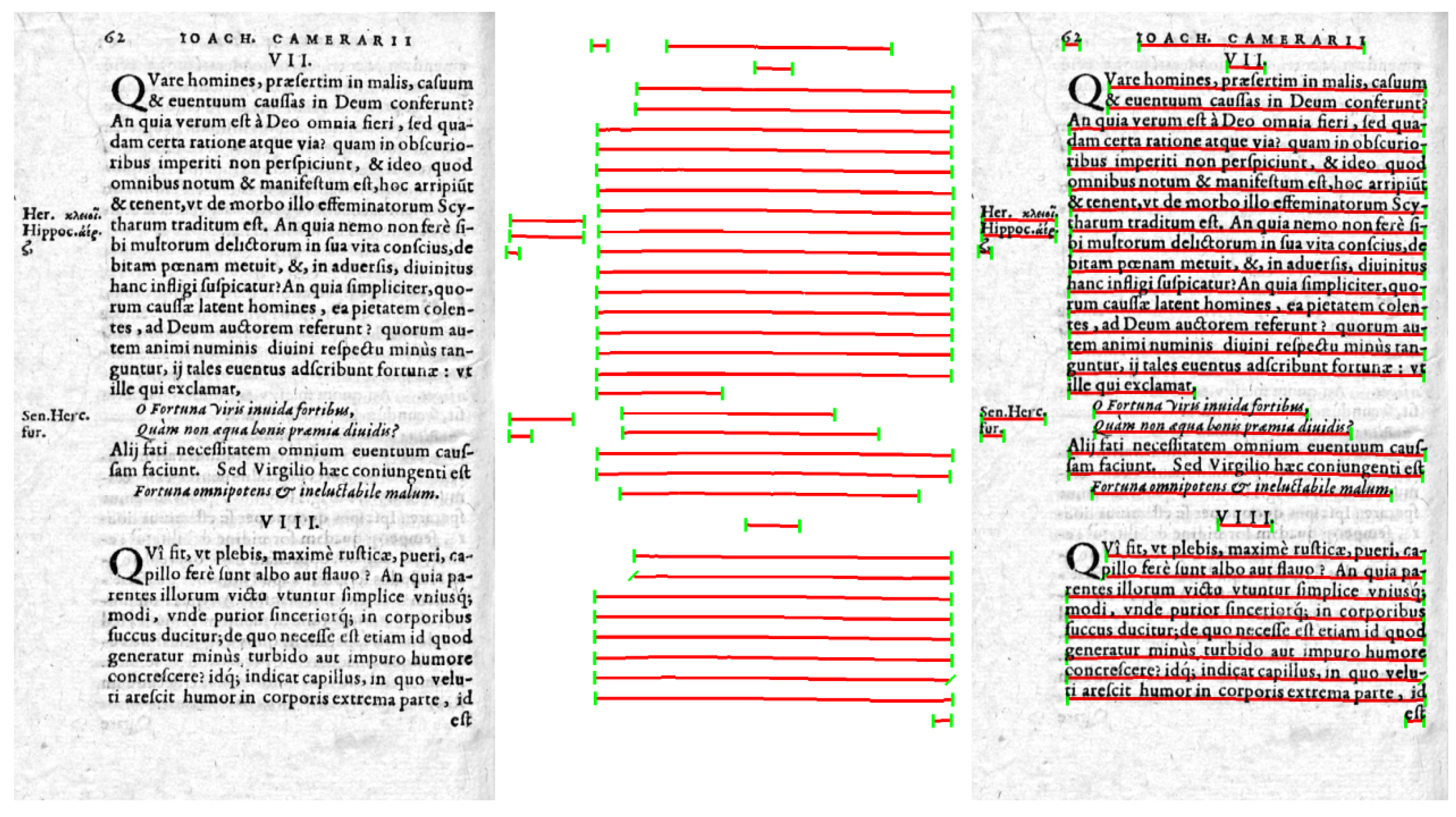
4.5. Polygonization of Detected Baselines
For the subsequent OCR step, baselines must be converted to line polygons, i.e., a list of points, whose connection defines the polygon. This is more precise than a simple rectangle in historic prints and should include all foreground pixels of all letters and punctuation marks of the text line in the binarized document image. Especially, when the inputs are scanned pages from books, warping can occur at the side of the page. In this case, bounding boxes cannot capture individual text lines precisely. In contrast, line polygons can follow the curvature of the line more precisely. For this task, we designed an algorithm that requires only the detected baselines and the binarized image as an input. The goal of our polygonization was to provide a robust output, even for slightly skewed or warped pages. An example of our algorithm is shown in
Figure 5.
First, the height of a text line was estimated based on the detected text lines above and below, with special estimations for the top and bottom lines. Since baselines may be too short or too long compared to the line above or below, a graph of the baselines was computed, connecting each baseline to its above or below baselines. A problem for baselines is the outer letters at the left and right side, which might be cut or connected to the next column in a naive approach. Therefore, we used a contour-based postprocessing step to compute the exact borders of the polygon of the baseline.
In the following, these steps are described in more detail:
Since the neural network only provides the baselines of the text line, we first estimated the x-height (the estimated height of a small character such as the letter x) in order to use it for the polygon generation. Since only a rough estimate for the following steps was needed, a simple algorithm was used. It moves up the baseline step by step in the binarized version of the image. In each step, the “black value” of the baseline is calculated, i.e., how many black pixels the baseline overlays. The highest value is saved. In addition, in each step, the current black value of the baseline is compared with the highest value. If the value is significantly lower, then we aborted and stored the number of steps used as the x-height of the line. Furthermore, we used a warm start for the algorithm so that it cannot abort after the first few steps. An estimated top line for the next step is generated by moving the baseline up by the determined x-height.
- 2.
Baseline graph generation:
In order to find other text lines that are above and below a given text line, a graph structure is utilized. In this structure, a node is generated for each baseline. Each baseline’s node is connected to another baseline’s node, if there is at least one pair of points with the same x-coordinate between the estimated top line of one node and the baseline of the other node, which are no further vertically apart than a given threshold. Therefore, each node is connected to another node, if their respective baseline or estimated top line is within a given “view window” of the other baseline’s estimated top line or baseline, respectively. Nodes that are found in the view window of the estimated top line are considered above the current node, whereas nodes that are found by their estimated top line in the view window of the current nodes baseline are considered “below” the current line.
- 3.
Top and bottom dividing line generation:
In order to generate the correct line polygon for a detected baseline, it is required to find the limits above and below the baseline. The top limit for the line polygon is composed of the joined baselines of the neighboring nodes above the current baseline’s graph node. In case there is a baseline above the reference baseline that overlaps the horizontal interval of the reference at least 80%, the joined top line is generated by interpolating the found baselines’ coordinates to extend the full interval of the reference baseline. If no joint estimated top line is found, the top limit is the estimated top line of the current detected baseline, moved again by its original distance to the top. The bottom limit is the joint estimated top lines of the neighboring graph nodes below the current baseline. If no joint bottom limit is found, the detected baseline is moved by 120% of the estimated height to the bottom. Then, the top and bottom dividing lines of the current line are generated. To generate either of these lines, we used the A* algorithm to find the shortest path from leftmost pixels between the top limit and the top line of the current baseline (or the baseline and the bottom, respectively) to the rightmost pixels. Edges pointing to black pixels are assigned a higher weight by the A* algorithm than edges pointing to white pixels. Therefore, the algorithm aims to cut around the contours of the individual letters in the line. This is especially important for documents with narrow spacing between the lines and big letters, where letters reaching far below the baseline in the line above and capital letters in the bottom line are sometimes touching and/or interleaving. Vertical steps are also slightly penalized, resulting in a mostly straight divider if the lines are sufficiently spaced apart.
In order to account for cases where no top or bottom limits could be generated from the baseline graph and the resulting top and bottom limits are approximations, a starting bias is added to the A* algorithm. For the top dividing line, the cost of the starting node is lowest at the bottom and increases consistently to the top. For the bottom dividing line, the cost of the starting node is the lowest at the top and increases consistently further down.
The resulting shortest paths for the top and the bottom of the line are then the final top and bottom dividing lines of the line polygon. The polygon is then given by concatenating the line segments of the top and bottom dividing line and inserting a segment on the left and, similarly, on the right that connects the first/last point of the top to the first/last point of the bottom line, respectively.
- 4.
Baseline extension:
In many cases, the predicted baselines do not underline the beginning and ending letter of the line fully. In order to improve the polygon generation, we extended the baselines to the left and to the right using the following heuristic: using the generated top and bottom lines, the height of the line is estimated to be the arithmetic mean of the distance between the top and bottom line. A rectangular box using a fixed width, the point in the baseline, and the estimated height is created to the left and the right of the baseline. In this box, we find the closest vertical scan line, which contains almost no foreground pixels in the binarized image. If such a scan line exists, the baseline is extended on the corresponding side. To account for a potential skew in the image, the vertical position of the new point is adjusted using the gradient of the original baseline. An example of this step is provided in
Figure 6. In case at least one baseline was extended, the last two steps of the polygonization are subsequently applied again to account for the changes.
- 5.
Fixing contours at the beginning and ending of the line:
To further reduce the risk of cutting off parts of a letter at both ends of the resulting polygon, we used a contour-based approach to further improve the polygonization quality. For this, we found all connected components in the binarized image. If the left or right segment of the resulting line polygon connecting the top to the bottom line intersects with exactly one connected component, the following steps were taken to determine if the line polygon should be extended to span the whole connected component: (1) The width of the connected component must not be larger than the average height of the text line. (2) The bottom of the CC must be below the height of the baseline, given a slack of 20% of the average line height. (3) The bottom line of the connected component must not be lower than the baseline, given a slack of 20% of the average line height. (4) The height of the connected component must not be higher than the average line height given a slack of 10%. (5) The contour must not be a valid candidate for other line polygons given the previous conditions. If all conditions are met, the line polygon is enlarged to be the union of the original line polygon and the convex hull of the connected components pixels.
4.6. Rule-Based Layout Analysis
The goal of the rule-based layout analysis is to assign a class label to the detected text lines using background knowledge and subsequently correct potential errors from the baseline detector, such as text line polygons that also span the marginalia to their sides. The algorithm consists of three main parts: The heuristic detection of text columns, a rulebook detecting line features, and a postprocessing step in which the detected features are used to correct lines and to assign the detected labels to the output lines.
The rules are applicable to a wide range of different historical prints with different layout types, incorporating rules for commonly found elements such as marginalia, header regions, or footers. In addition, the user can add or overwrite rules for a particular historic print.
4.6.1. Heuristic Column Detection
This step aims to detect the number of columns on a page. All starting and end points of the text lines are extracted to compute the main text blocks on the page. We define a text block as a set of lines, which are directly above or below each other. As a text block must not span multiple columns, text blocks cannot contain lines that have more than one line above or below them. In order to find such blocks, a directed graph structure is used (see above), where text lines are connected by edges to text lines below, if their bounding boxes are at most half of the average line height apart vertically, and their horizontal intervals are intersecting. Text blocks can then be extracted by finding subsets of nodes in the graph that have at most one incoming and one outgoing edge.
Next, a heuristic is used to determine the maximum number of columns on a page: A page is considered to have a two-column layout if there are two horizontally adjacent text blocks, whose bounding boxes overlap at least 50% vertically and whose widths sum to at least 40% of the page’s width. If no such text blocks are found, the page is assumed to only contain one main text column. For our method, we assumed that the page spans the whole input by the width. Although this is certainly rarely the case, the parameters were set conservatively to allow for a margin of error. For practical purposes, it can be assumed that the width can be determined from the metadata of the page’s scans or the print’s physical dimensions and the DPI of the digital copies.
In order to heuristically detect the horizontal intervals of the text columns, the beginning and ending points of all detected text lines were clustered using the k-means algorithm. The number of cluster centers was set to one more than the heuristically determined number of main text columns. The x-coordinate of the column dividers was then determined to be the median of the x-coordinates of each cluster’s points.
If a two-column layout was detected, a postprocessing algorithm is used to fix the column divider of the main text blocks. In this case, we determined the lowest x-coordinate of all text lines starting right of the divider and the highest x-coordinate of all text lines ending before the divider. If such coordinates were found, the divider was set to the average of both coordinates. If only one coordinate was found, the divider was set to that coordinate.
Finally, each detected line is assigned to a column if its center lies inside the column interval. Lines reaching over multiple columns, such as marginalia that were not separated, are not detected as such in this step, but rather using a rule from the rulebook (see below).
In addition, lines are grouped into individual rows. Two lines are determined to be on the same row if their center point is further apart vertically than a third of the median of all detected text lines’ heights.
4.6.2. Individual Rules in the Rulebook
After the column intervals were found, the following rules were applied consecutively to the detected lines of the page:
If two columns are detected, the average length of lines strictly inside the column is determined. If the average length of the lines in one column is greater than 1.8-times the average length of lines in another column, then the column container of the shorter lines is labeled as a marginalia column. If three or more columns are found, the outside columns are labeled as potential marginalia columns.
Lines reaching across multiple columns as a result of an error in the baseline detection are detected. Each line whose horizontal interval overlaps with at least 1/20th of one or more of its neighboring column’s interval on either side is labeled to be contained in that column, if that line is at least 80% as wide as the neighboring column.
Each line completely inside a marginalia column interval is labeled as a marginalia. For lines that are not completely inside a marginalia column, but also do not reach across multiple columns, are also counted as marginalia if they are approximately on the same row as another line, because marginalia are commonly found next to other text lines. In addition, the lowest line on the page is skipped, as this might be a potential catchword or signature mark that is printed far to the right. As another constraint, a line cannot be labeled as a marginalia, if it is wider than a third of the page width.
The user can add a configuration that the top line of a page is a header (i.e., metadata) or a headline (i.e., text). Otherwise, the following rules are applied to the top line:
If the height of the line is higher than 150% of the median of all lines on the page and it is centered compared to the main text columns, it is a headline.
In some historic books, the printer decided to save space by printing a headline and a page number (header) in the same line. Therefore, we needed a special rule to separate both parts. The user must state such a situation with a configuration. The rule is only applied if the topmost line on a page is either reaching further to the right or left as all the remaining text lines or if the header is wider than 33% of the width of the main text area. Then, the cut point is computed as follows: For each x-coordinate in the line, a window with a fixed width is extended to the left and the right of the point. The sum of all foreground pixels for each vertical slice of the polygons bounding box in the window is calculated and weighted by the distance from the window’s center. The cut point is determined by the x-coordinate with the lowest weighted sum of foreground pixels in its window. This method ensures that the polygons are cut in the middle between the headline part and the header part, independent of the width of the header or headline. Otherwise, the default rule is to assign a header.
Footer elements may be catchwords or signature marks in the bottom line of a page. Again, the user can state a configuration that the bottom line of a historic book is always a footer or not. Otherwise, the following two rules for the bottom line are used to detect footers, which may be composed of multiple elements:
If the bottom line is not inside the leftmost or rightmost column interval of the page and if the horizontal distance between its bounding box and the right limit of the column interval is less than half the width of the line’s bounding box, it is a footer.
If there is a line in the same column in the row above the bottom line, its width is less than 40% of the above line’s width, and it is indented by more than 20% compared to the above line, then the bottom line is a footer.
4.6.3. Segmentation Postprocessing
After the rule-based layout detection has run, the results are used to improve the segmentation. First, if lines have been marked as spanning multiple columns and one of those columns has been detected to be a marginalia column, the line might be split in order to separate the marginalia from the text line.
For this, the optimal vertical division is calculated. A heuristic is applied to find congestion points on the page. A congestion point can be seen as a point between two horizontally adjacent lines that are nearby. If two lines are horizontally adjacent to each other and their endings are not further apart than 20px, a congestion point is added. The detected points are then greedily grouped by their x-coordinate to form clusters. If there is one of those clusters found, a text line spanning into a marginalia column is cut at the x-coordinate of the closest congestion point found. In case no such points could be discovered, e.g., on pages that only contain a single marginalia, the detected vertical column divider is used.
For pages where a multi-column layout was detected, there might exist text lines spanning multiple main text columns, as the baseline predictor does not separate the baselines in some cases.
In this case, all lines that have been detected to span such columns are cut at the position of the detected column divider, unless they have been detected to be of a different type than normal text, such as header or footer elements, or significantly bigger headlines.
For the header and footer class, a special postprocessing step is taken to merge individually detected elements: If more than one header or more than one footer was found, the polygons of the respective class are merged into a single polygon of that class. The merged polygon is given by the convex hull of all points of the polygons.
If any line was cut, all rules are applied again to the page in order to improve the column divider detection and to assign the correct classes to the newly generated lines.
5. Evaluation Scheme and Metrics Used
For the evaluation of the baseline detector and subsequent line polygonization, we used two different metrics. First, we evaluated individual foreground pixels in the document images. A foreground pixel was counted as a TP if it was contained in a prediction text polygon and a GT text polygon, an FP if it was only contained in the prediction, and likewise, an FN if it was only contained in the GT. Using the TP, FP, and FN, we calculated the per-pixel text precision, recall, and F1-score.
In order to evaluate the accuracy of the generated text polygons for the OCR step later in the pipeline, individual instances of detected page elements (e.g., text lines and dropped capitals) were evaluated. Therefore, we used the following metric: Each GT page element was matched to its best-fitting predicted page element using a maximal bipartite matching using the intersection over union (IoU) measure on the foreground pixels of the predicted and ground truth polygons as a distance function. The polygon was counted as detected if it matched with a GT polygon with an IoU score of or higher. For small elements (elements that are not wider than 10% of the page’s width), an IoU threshold of was used. A detected polygon was counted to be of the correct type (“correct”) if its class label matched the label in the ground truth.
Based on the correctly classified polygons, we calculated the precision (prec) and recall (rec) for each class, counting correctly predicted elements as true positives, undetected ground truth elements as false negatives, and other predicted lines of that class as false positives.
In addition, we evaluated if the line endings of the detected elements matched a GT polygon. The line endings were counted as correct if the left and right side of a detected polygon and its best-fitting ground truth polygon did not differ by more than a given threshold (1%) of the page’s width (disregarding white space on either side), which is approximately half the width of a character for the 1% threshold. Therefore, line ending accuracy describes the fraction of detected polygons with correct line endings among all detected GT elements of a given class using a certain threshold.
We argue that this measure is more representative for the evaluation of detected text elements on a page than other commonly used measures, such as the FgPA [
10] or the mIoU metric [
11], as even small errors at the beginning or ending of a detected line polygon can negatively affect the subsequent OCR step and lead to incorrectly recognized or missing characters. The fact that many lines end with a hyphen or punctuation strengthens the negative effect, as such characters are small and, therefore, contribute even less than regular characters to the overall score in the metrics such as the mIoU or per-pixel accuracy.
6. Experiments
6.1. Text/Non-Text Segmentation and Text Line Instance Segmentation
We conducted an experiment to compare the results of our text/non-text separation and the text line instance detection to the open-source OCR software Kraken [
23]. For this, we trained a model for the Kraken text line detection using the default parameters on our main training set and fine-tuned it using default parameters on our fine-tuning dataset, similar to the training method of our baseline detector, as described in
Section 4.3. It has to be noted that we only trained Kraken on the baselines, as the training datasets do not contain further annotations for region or text line classes.
For the per-pixel evaluation, all text lines as predicted by the Kraken segmentation were counted as text line polygons. Pages, which could not be processed by Kraken, have been left out of the evaluation in favor of the Kraken system. For the per-pixel evaluation of our methods, only the text classes (text, column, marginalia, header, and footer) were counted. We report the results of our method with and without the manual user configuration.
For the text line instance segmentation, we used our evaluation scheme as described in
Section 5. As the Kraken engine was only trained on the baseline and no region types, we removed the class segmentation in this experiment and counted all text classes in the ground truth as a single class.
The results for this experiment are presented in
Table 2 for the Kraken engine and in
Table 3 for our method.
6.2. Layout Recognition
For the evaluation, experiments were conducted on the five datasets described in
Section 3.1 with the goal of detecting all text elements with their types as described in
Section 3.2. We used both a standard configuration, which is sufficient for a simple layout, and a book-specific configuration, where we could enable or disable the recognition of certain features. Such configurations are different from book-specific training, where the annotated GT for a new book is necessary. Instead, the manual interventions concerned only Boolean values. Currently, the settings that can be adjusted by the user are:
Specifying if one or two main text columns are in the given print (default = heuristic determination of the number of columns);
Specifying if marginalia are absent in the print;
Specifying if dropped capitals are absent in the print;
Specifying if headlines are contained in the page header.
We repeated the features of our five datasets and state if the configurations were performed and were evaluated:
Single-column layout, no marginalia, single header and footer element per page, few dropped capitals, no images.
Single-column layout, marginalia on left and right side, composed header and footer element per page, few dropped capitals and images.
Two-column layout, mixture of headline (i.e., text) and header (page number) in the top line, which must be separated, single footer (sometimes on the same line as text), many images, no dropped capitals, no marginalia. Text lines have a ragged right side. Some degradation, i.e., small parts of a page are missing.
Single-column layout, marginalia on left or right side, single header and footer per page, many images, no dropped capitals. Text lines have a ragged left and right side, and marginalia also have a ragged right side.
Single-column layout, marginalia on left and right side, single or composed header and composed footer, 102 dropped capitals, and one image. Handwritten elements such underscores and symbols similar to marginalia are present.
The datasets CamStd and CamMarg were evaluated with the standard settings without special configurations. This holds true for CamManual as well, although a configuration stating that there are manual artifacts would have been beneficial; however, currently, we have not implemented special routines for dealing with artifacts. In the other two datasets, in addition to the standard setting, a book specific evaluation was added with the following switches:
The number of columns was manually set to two, and marginalia and dropped capital detection were deactivated. Additionally, we applied a rule that classified centered headers as text elements instead of headers.
The experiment was performed with the dropped capital detection disabled.
All experiments were performed using a single baseline detector and dropped capital detector model, which were trained as described in
Section 4.3 and
Section 4.4.
7. Evaluation Results
The evaluation of our text/non-text pixelwise segmentation in
Table 3 showed that the text elements on the page were almost fully recognized, with a macro-averaged per-pixel F1-score of
. When compared to the results of the Kraken engine, which achieved a macro-averaged per-pixel F1-score of
on our datasets, this showed that our method provided a slightly improved text recognition on the tested datasets.
When comparing the text line instance segmentation performance, our results showed a clear improvement with a macro-averaged F1-score of with the default settings compared to for the Kraken system. Especially on the GW5051 dataset, which features a two-column layout, the results showed the highest difference between the two methods. A review of the results suggested that Kraken often failed to separate nearby text lines such as marginalia from the main text or merged the lines from the two columns.
The evaluations for the layout recognition followed our evaluation scheme as described in
Section 5. The results, as presented in
Table 4, were all achieved using the same baseline detector model. The detailed evaluations require knowledge for splitting or merging the baselines and the classification of the text lines types. As described in
Section 2.3, we used general background knowledge and special configurations about the existing layout types for each dataset representing one book or several books printed in the same layout. Our default configuration was an automatic column detection with marginalia, a header and a footer line, and dropped capitals and images.
The configurations used for the datasets were:
CamStd: no changes to the standard configuration;
CamMarg: no changes to the standard configuration;
GW5051: two-column layout, no marginalia, no dropped capitals, split of the top line into headline and header;
GW5056: no dropped capitals;
CamManual: no changes to standard configuration.
The main results can be summarized as follows:
CamStd: nearly perfect layout recognition;
CamMarg: confusion of the very few dropped capitals with text elements, nearly perfect normal text lines’ recognition, and good footer, header, and marginalia recognition (between 97.5% and 99.0% precision and recall);
GW5051: very good column separation (precision 99.8%, recall 99.9%), some problems with footers (due to very short footers causing problems for the baseline detection), and good results for separation of the top line into header and text (headline);
GW5056: very good results for the separation of marginalia and text (despite ragged side), good results for header, and similar to GW5051, some problems with footer due to very short footers;
CamManual: overall good results despite difficult layout and dropped capitals, as well as unexpected elements (handwritten artifacts and underlines, astrological symbols).
In total, our method achieved a macro-averaged F1-score of for all text line instances averaged across the datasets and different classes. For the dropped capitals, which belong to the non-text class, an F1-score of could be achieved on the CamManual dataset.
8. Analysis of Commonly Occurring Errors and Discussion
In this section, we analyze commonly occurring errors in the predictions. The number of occurrences of these errors were counted for the CamStd, CamMarg, GW5051, and GW5056 datasets manually, using the visualizations provided by our evaluation script. The results of the analysis are presented in
Table 5.
Our evaluation for the layout recognition shows, in
Table 4, that overall, we achieved good results on the tested datasets. Especially, it has to be noted that, for all datasets, all main text line instances were located by our baseline detection method for the analyzed datasets. In general, the main text line detection errors were the result of missing parts due to erroneously detected marginalia cut locations, falsely detected dropped capitals, missing letters at the beginning or endings of the line, or incorrect column separation. Some elements, such as marginalia, small headers, or footers, can be observed to be missing entirely from the baseline prediction and, therefore, the resulting segmentation, as explained in detail in the following. In some cases, additional baselines were detected, such as parts of images, background noise, or degradations, which resulted in false positives in the different text classes, depending on their location on the page and their classification by the rulebook.
On the CamStd dataset with no marginalia and a standard layout, almost all elements were successfully detected and no additional lines were present in the prediction, except for two text lines, which were mistaken for headers.
On the more complex CamMarg dataset, the results showed that the main page layout was, in all cases, successfully detected as single column as no column classes were predicted. Only five main text lines were not detected, which was the result of inaccurate marginalia cuts or dropped capitals predicted in the text region. The line endings were also correct in more than 99% of the cases, except for the marginalia class, where sometimes, missing asterisk marks in the front led to the line endings being incorrect. More than 97% of the marginalia regions were detected correctly. As the marginalia are often printed in small letters, background noise from the binarization can lead to an inaccurate polygonization, leading to small errors at the beginning and endings of the marginalia. As the difference between the line ending accuracy with the
threshold suggests, these errors were small, often less than the width of a single letter. The error analysis in
Table 5 showed that only one of the detected marginalia was incorrectly cut. The main errors concerning marginalia in this dataset were that 11 marginalia were not predicted at all by our baseline detector due a too small size. For the header category, three segmentation errors occurred, when page numbers were not detected by the baseline detection, and therefore, the header polygon was too small, missing a significant part.
Furthermore, the dropped capital detection predicted all existing dropped capitals in the CamStd and CamMarg datasets correctly. In the CamMarg dataset, three additional dropped capitals regions were incorrectly predicted in text lines, which led to errors at the beginning and ending of those text lines. In the future, these false positives could be eliminated by applying rules for the postprocessing of the dropped capitals, e.g., by utilizing information from a subsequent OCR to detect that characters from the words are missing.
Furthermore, the evaluation on the CamStd, CamMarg, and CamManual datasets suggested that, for single-column layouts, our detection heuristics worked.
For the GW5051 dataset, it can be seen that the columns were, in most cases, successfully detected. In all cases, it was successfully determined that the columns should be separated. Only in 34 instances were two columns not separated exactly and part of the text in the column was cut. In addition, using the special rule for cutting the top line into the header and headline (text), only 4 out of 67 folio numbers were not correctly segmented. This could in particular be further improved by an OCR, as the folio numbers consist of Latin numerals and could, therefore, be distinguished from the text in the headline. Furthermore, as our header rule only applies to the top line, it can be seen from the error analysis that, if noise is detected as text above the top line (in one case in this dataset), the header cannot be detected and, therefore, is not be separated from the headline. In addition, the dataset contains signature marks on the same line as the last text line, which we did not expect and is, thus, not covered by the rulebook. This led to one footer element not being detected correctly, as it was not separated from the main text in the same column. Furthermore, some footer elements were not detected, as they were very small and, thus, not recognized as text by our baseline detector. In addition, two text elements, which were printed similarly to footers, were falsely detected as footers in this dataset, which we believe could only be detected by using the transcription provided by the OCR.
The evaluation of the GW5056 dataset showed that, although the main text lines had ragged left and right edges, the main text was still detected successfully for the most part as 99.6% of the text lines were detected, out of which 99.7% had accurate line endings. Five of the detected text lines were incorrectly classified as headers, because no header was present on these pages and our rules were built on the assumption that a header is present on every page. As the error analysis showed, the marginalia were detected in more than 98% cases with only one instance, where the marginalia were detected as header elements, as the header element was not detected on that page. The error analysis showed that there were only 8 instances where marginalia were not separated from the main text and 18 instances where the separation was inaccurate. Although many footer elements in the dataset consisted of spaced individual letters, it can be seen that these were accurately detected, but only 26 out of 28 were predicted to be of the footer class.
Additionally, it can be seen that 2 and 6 text lines were erroneously detected in image regions in the GW5051 and GW5056 datasets, respectively. In the future, this could be improved with a postprocessing step by also detecting the image regions, e.g., using an object detector such as a Mask R-CNN, similar to our dropped capital detection.
The evaluation of the additional CamManual dataset showed that, even though handwritten annotations and artifacts were present, the main text was detected more than of the time. For the header category, similar errors as in the CamMarg dataset can be observed, as sometimes, small page numbers were not detected. In addition, many marginalia regions in this dataset were very short, often consisting of a single astrological symbol. Only of the marginalia regions were detected. In addition, handwritten artifacts were often detected as marginalia or interfered with the marginalia separation.
As this dataset contains significantly more dropped capitals than our other datasets, it is important to mention that, out of the 102 dropped capitals, 96 were correctly detected, and the width of the detected elements was always correctly predicted (using a threshold of ). A review of the results showed that most false positive dropped capital predictions occurred at the beginning of lines (similar to the CamMarg dataset), which led to these lines not being fully detected or at black spots (degradations) in the middle of a text block. As previously stated, the precision of the dropped capital detection could be improved in the future by incorporating the results from the subsequent OCR or by applying feedback from the layout analysis in a postprocessing step for the dropped capital detector. The header category also showed similar issues as in the CamMarg dataset, with headers often missing the page number. For the footers, the errors were also similar to the CamMarg dataset, with most of the footers correctly detected, but sometimes not classified correctly as a footer element.
To conclude the analysis of our results, it can be stated that most observed errors only affected individual lines (or two lines in the case of separated marginalia/columns or headers). This can be seen as an advantage of our method, as such errors are easy to correct manually, together with the subsequent OCR step. Furthermore, slightly incorrect line endings must not be corrected at the segmentation level at all, but can be corrected in the OCR step, where it could even be possible to highlight some of these errors, as the resulting OCR contains partial words that are not found in a dictionary.


