1. Introduction
Connected-component analysis (CCA) is a common problem in many imaging applications, such as medical imaging [
1,
2], automated quality assurance [
3,
4] or real-time automotive applications [
5,
6]. A novel application is image-based process control using ultrafast electron beam X-ray computed tomography (UFXCT) [
7]. UFXCT is a non-invasive imaging technique yielding up to 8000 images per second. This image stream is reconstructed and processed in real-time on a GPU using the so-called Real-time Image Stream Algorithms (RISA, [
8,
9]) framework. CCA shall now be used in RISA to extract object features from this reconstructed image stream. Based on these extracted features, the UFXCT scanning position is adapted during scanning to track moving objects, e.g., a rising gas bubble in a liquid column. For stable tracking, features must be extracted within a latency of at most 5 ms [
10]. Consequently, the connected-component analysis in RISA must also be performed in an efficient and computationally cheap manner on the GPU. After the analysis, resulting features must also be transferred to the host for long-term storage and possible further analysis. Lastly, the connected-component analysis should be implemented as a separate processing step independent of the labeling to maintain maximal flexibility, e.g., when pre-processing of the labels is required. One such example is the aforementioned analysis for UFXCT which requires persistent labels for the same logical object between consecutive frames. Note, however, that RISA can be applied for general purpose image stream processing and is not limited to UFXCT. However, we will use UFXCT as an example application for introducing the design of our CCA algorithm because it imposes the most strict constraints (latency, label persistence).
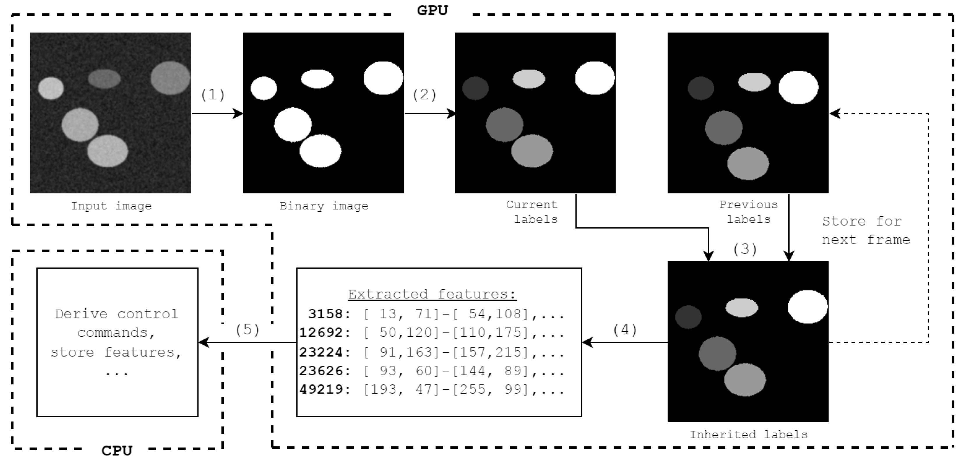
Given these constraints, CCA for UFXCT can be divided into the steps shown in
Figure 1:
- (1)
Image binarization (e.g., using a global threshold);
- (2)
Connected-component labeling (e.g., using the algorithm developed by Playne [
11]);
- (3)
Label inheritance [
12] for objects which are visible in multiple consecutive frames;
- (4)
Feature extraction with our proposed tree merge kernel (see
Section 3.2);
- (5)
Transfer of these features to host memory for storing and further processing.
In this work, we focus on the connected-component analysis. Related work is described in the following
Section 2.
2. State of the Art and Related Work
In the context of this paper, we define the connected-component analysis problem such that connected regions of foreground pixels in a binary image (“true”), representing logical objects, are labeled identically. For each of these objects, a set of properties, like overall area, centroid position and bounding box, is to be extracted. To solve those problems, many algorithms were already developed which can be coarsely classified into sequential (e.g., [
13,
14,
15]) and parallel algorithms (e.g., [
16,
17,
18,
19]). In this paper, we will focus on parallel implementations of connected-component analysis (CCA) for execution on NVIDIA GPUs. Note that many approaches for CCA use hybrid kernels which label and analyse the components in a single step (e.g., [
16,
18]). This approach is not applicable in our case due to the inheritance constraint. However, these algorithms can typically also be applied to a labeled image which allows us to compare their performance with our own implementation.
A major issue for any parallel CCA implementation is that multiple independent processes may try to update the same component’s features concurrently. Resolving this typically involves using atomic instructions which serialize any memory accesses to maintain a well-defined state. However, serializing the process counteracts the initial idea of increasing performance by executing operations in parallel when using GPUs.
To circumvent the serialization, different approaches were already developed. HA4 [
16] is an algorithm especially designed to circumvent slow-downs due to ineffective hardware usage (e.g., non-optimal memory accesses). It uses a single thread per image row which traverses the image column-wise. Labels and features can be updated in the same iteration using specific warp-level primitives yielding very good performance. Similarly, [
19] further reduced possible causes for serialization due to merging conflicts between threads. This is achieved by using on-the-fly feature merges or conflict detection, again, implemented with low-level CUDA functions.
With these performance improvements, transfer time from device to host increasingly dominates overall execution time when feature processing on the CPU is required. The CCA approaches introduced above do not consider reduction of transfer volume. Instead, a set of arrays (one per feature) is filled by the CCA algorithms typically yielding sparsely populated arrays. Naïvely transferring these to the host leads to longer transfer durations and increased computing costs on the CPU to iterate and process a large set of empty or invalid array entries.
In our contribution, we introduce CCA based on a tree merging algorithm which creates a tree structure whose root node contains the size of the total tree. Hence only valid property blobs are downloaded from the device to host memory drastically reducing the transfer volume for most use-cases.
3. Materials and Methods
3.1. Boundary Conditions for CCA in Image Stream Processing
The proposed algorithm was developed with these design considerations stemming from its application in image stream processing:
Image contents between consecutive images are assumed to contain approximately the same number of objects.
Object features need to be transferred to host memory for storing or further processing.
The data processing framework (RISA) may require large portions of the available memory bandwidth for copy operations between host and device memory. The CCA algorithm should therefore use minimal memory bandwidth.
Applications may require pre-processing of labels before the feature extraction. Hence, CCA must be performed as a separate step and not during the initial labeling process.
3.2. Tree Merge Kernel
Consequently, the proposed Tree Merge Kernel (TMK) consists of these steps:
- 1.
Initialization;
- 2a.
Tree merging (in shared memory);
- 2b.
Tree merging (in global memory);
- 3.
Updating tree size information;
- 4.
Tree balancing.
Given a labaled image, the developed algorithm computes a binary tree of object feature structs (OFS) which are stored in a contiguous array (F). Each OFS includes information about the object itself (label, number of pixels, boundary box, sum of coordinates x, sum of coordinates y) as well as the tree structure (parent index, left and right child indices, total number of child nodes). Each OFS can therefore be interpreted as a tree node. After balancing the tree, all the valid nodes are moved to the beginning of the array. This allows us to transfer only the valid nodes at the beginning of the array to the host in a single copy operation, which we assume to lower required memory transfer bandwidth.
The steps to build this tree structure are detailed below. For the code shown, we define these variables: F = array of object feature structs, INVALID_LABEL = constant value indicating a pixel is not a foreground pixel, L = array of image size containing one label per pixel, tig = thread index in the grid used when calling the kernel.
3.2.1. Initialization
The input to the algorithm is a labeled image of size width · height = numPixels pixels. This image can contain at most numPixels/2 = maxNumObjects distinct objects (i.e. a chessboard pattern) because two neighbouring foreground pixels can not be part of different objects. If they were touching, they would be considered the same object. Hence, we can initialize the feature extraction allocating an array F of size maxNumObjects OFSs. In the initialization kernel, we use maxNumObjects threads which initialize F by processing two neighbouring pixels as shown in Algorithm 1.
| Algorithm 1: initialize(F, L, width) |
![Algorithms 16 00080 i001]() |
F then contains maxNumObjects OFSs which are initially disjointed tree nodes. Each node either holds a valid tree (when at least one of the associated pixels is a foreground pixel) or an invalid tree (when none of the associated pixels are foreground pixels).
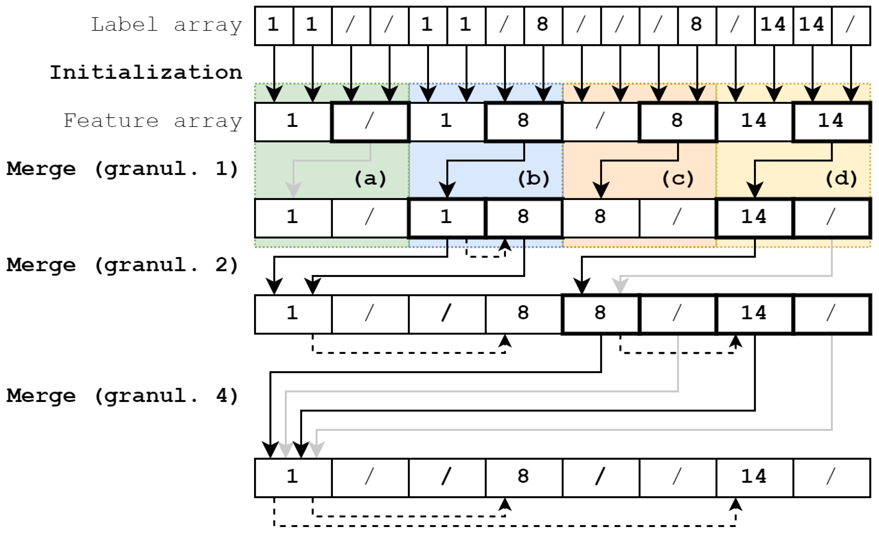
3.2.2. Tree Merging
These initially independent trees are then iteratively merged with doubling granularity between iterations. Trees are merged in shared memory first. If the granularity exceeds the shared memory capacity, the resulting trees are then finally merged in global memory. As shown in
Figure 2, each active thread (boxes with bold outline) handles two tree nodes per iteration in one of four scenarios (colored boxes):
- (a)
The source node is invalid, i.e., empty. The target node therefore remains unchanged and the assigned thread returns.
- (b)
The source and target node contain different labels. The source node is inserted as a child node into the target tree (as indicated by the dashed arrow). Note that this insertion is performed using atomicCAS to prevent multiple threads from claiming the same empty spot in the target tree.
- (c)
The target node is invalid and therefore replaced by the valid source node. The source node’s children are updated with the new parent address.
- (d)
The source and target node are labeled equally and are merged by updating their features. Because a label cannot occur twice in an existing tree there are no merging conflicts, hence feature updates (e.g., min/max of coordinates) are calculated non-atomically. Existing pointers to child nodes are removed to prevent conflicts. These cut-off child nodes are inserted back into the tree by their respective thread in subsequent iterations.
Between the iterations, the threads need to be synchronized using __syncthreads when working on block level and cooperative_groups::this_grid().sync() when working on global scope.
3.2.3. Updating Tree Size Information
After building the tree, the size of each node, i.e., the total number of respective child nodes, is calculated. Updating the size information during building the tree would require propagating size increments atomically multiple times. Instead, we are opting to update the tree sizes after building it by assigning one thread per leaf node. This way, the minimum number of threads (one per object) perform the size updates reducing atomic instructions. As shown in Algorithm 2, one thread per leaf node traverses the tree up until the root whilst updating the size of each visited node. If the visited node has two child nodes, the size update is performed atomically using atomicCAS. When only one child node is present, the update is performed non-atomically.
| Algorithm 2: updateTreeSize(F, maxNumObjects) |
![Algorithms 16 00080 i002]() |
3.2.4. Tree Balancing
After updating the tree sizes, the valid tree resides in the sparsely populated array F. To maximally shrink the data volume before transfer to host, all valid nodes are shifted to the beginning of the array essentially balancing the tree. With the total number of valid nodes known in the root node, the host can now copy only the valid nodes located at the beginning of the array. The algorithm for this balancing is shown in Algorithm 3.
| Algorithm 3: balance(F) |
![Algorithms 16 00080 i003]() |
Note that the information about the total number of nodes resides in GPU memory. To copy the correct amount of nodes, i.e., at least all valid nodes, it is assumed that the number of objects does not change drastically between consecutive frames. Initially, a user-provided number of objects is downloaded. It can then be checked if all valid nodes were copied by accessing the size of the root node in host memory. If not all nodes were copied, the remaining nodes are transferred in a second copy operation. In consecutive frames, the number of nodes in the previous frame (plus a safety margin) is copied in the first copy operation. If the assumption of roughly constant number of objects holds true, this will eliminate the necessity for the second copy operation whilst also only copying a fraction of the feature array F.
3.3. Performance Evaluation
We benchmarked the performance by executing a processing pipeline in RISA consisting of three stages:
A “loader stage”, which loads the respective part of the benchmark data set into device memory and sends it out in fixed intervals;
A “connected-component analysis stage”, which consumes the data stream from the benchmark loader and performs CCA (including labeling using Playne), and finally forwards the labeled images for further processing;
A “discarder stage”, which removes images from the pipeline.
For a comparison to a state-of-the-art CCA algorithm, we also implemented the hardware accelerated 4-connectivity algorithm in the CCA-stage as outlined in [
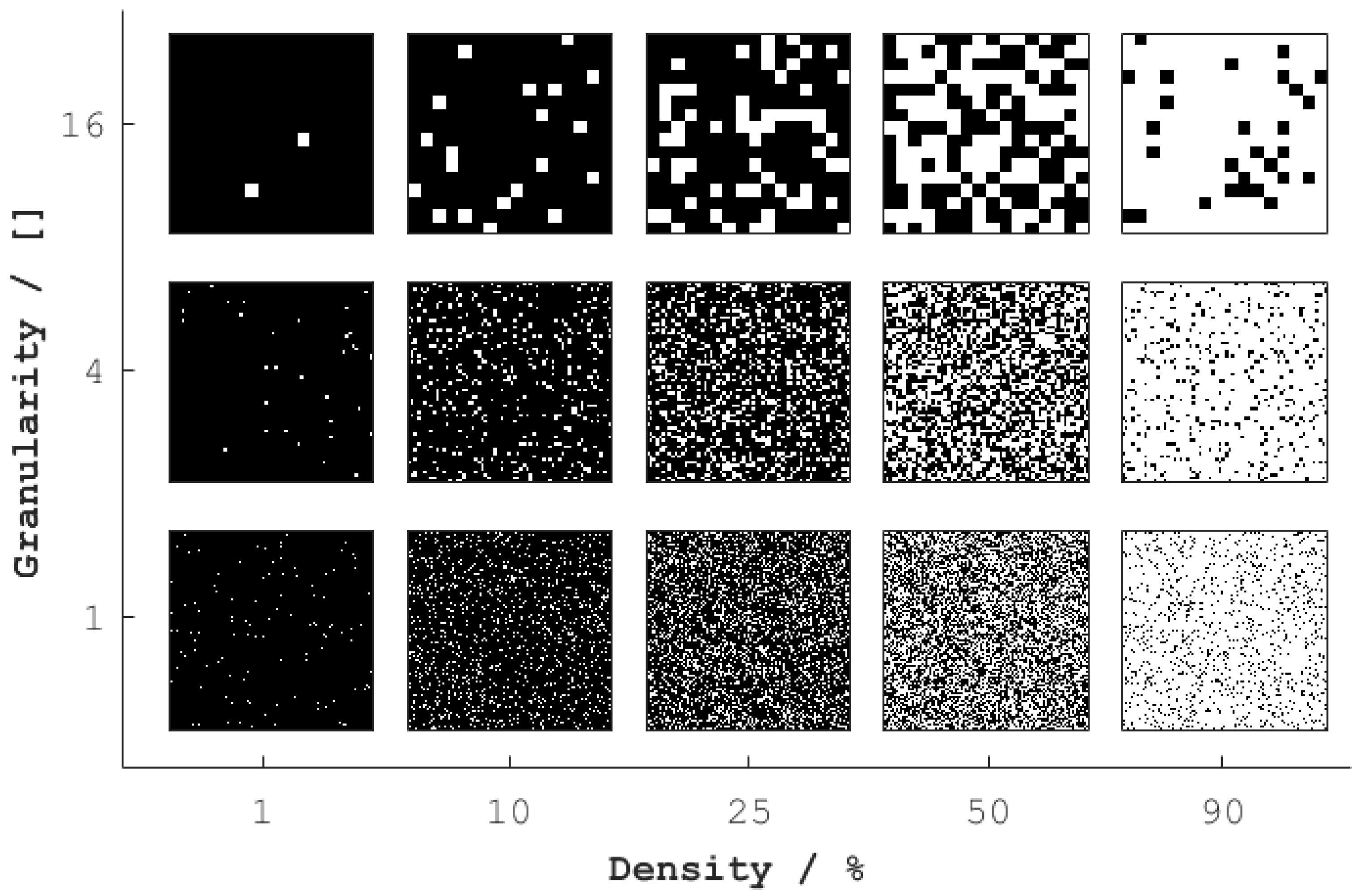
16]. We used the YACCLAB data set [
20] for our tests. This dataset contains a set of benchmark images from different applications which have been used for benchmarking CCA algorithms in different studies. In particular, we used the “random/granularity“ and “random/classical“ data sets (see example images in
Figure 3). The benchmarks were run on the two systems described in
Table 1.
Each benchmark was run by reading the set of ten images of the particular parameters (e.g., density 50%, granularity 4) into the device memory. This set is streamed through the processing stage repeatedly until 1000 images are processed in total. Using ‘nsys’, we assessed the kernel execution and memory transfer (device to host) durations.
4. Results
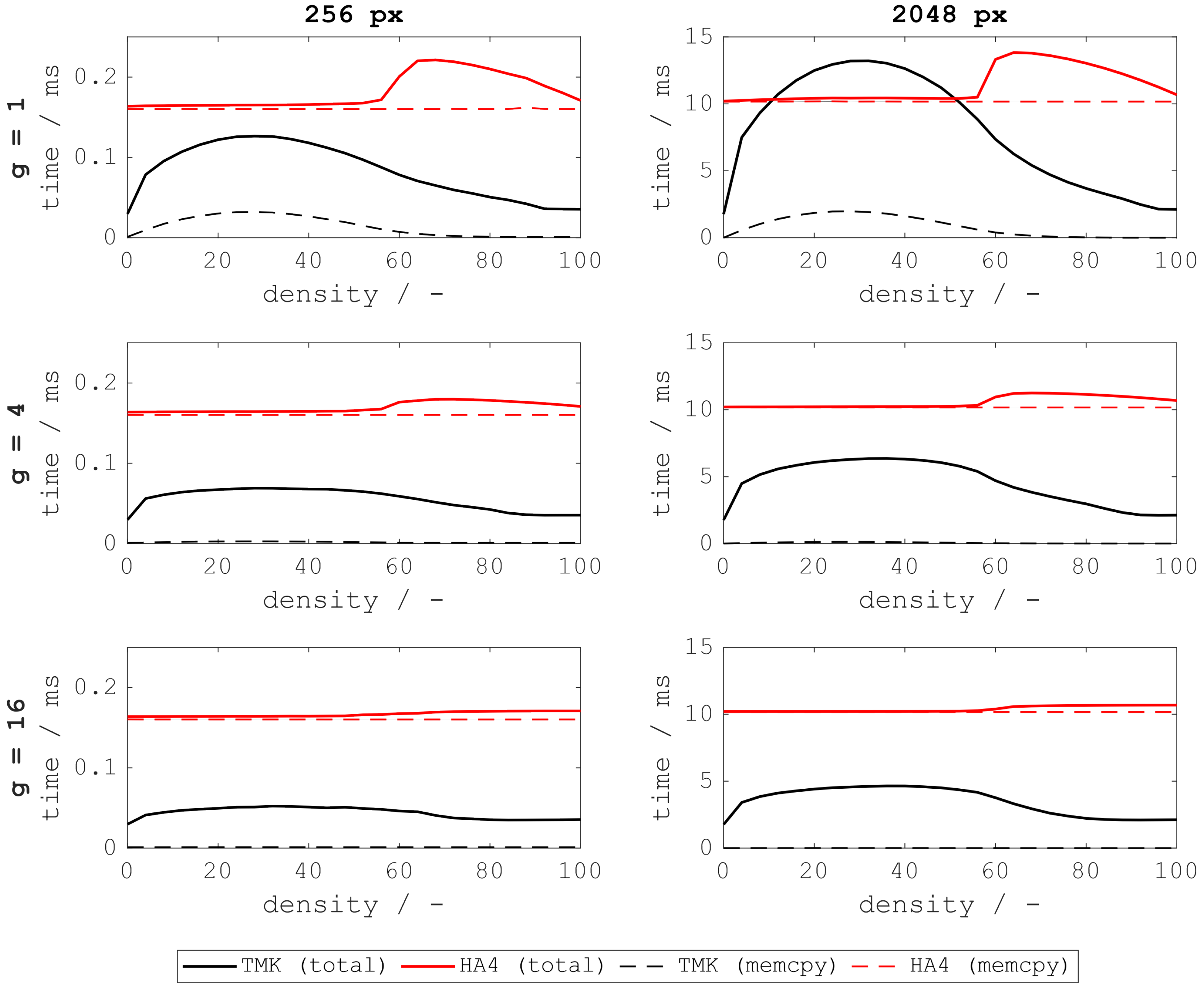
Figure 4 shows the execution times on the System A for the proposed tree merge kernel (TMK) compared to the HA4 algorithm. Benchmarks on the System B showed qualitatively similar results and are not shown. Note that the execution time for TMK includes generation and balancing of the tree, whereas the HA4 algorithm does not create a tree structure. Instead, the features array
F is filled and transferred completely. The results show that the increased computational effort on the device, i.e., building and balancing the tree, yields an overall lower execution time due to the drastically reduced memory transfer time in most cases.
Further, it can be seen that the tree merge kernels execution time scales with the total number of connected components rather than the number of foreground pixels, i.e., density. Hence, it performs worst for densities around 25% which yield the largest number of objects in the random images. Contrary, the tree merge algorithm remains unaffected by the percolation threshold around 60% which typically poses a bottleneck for CCA algorithms like HA4. This slowdown for algorithms like HA4 is a result of the sudden increase in object sizes at the percolation threshold. This leads to more conflicts between threads voting on the objects properties which need to be serialized. TMK, on the other hand, merges object properties non-atomically (as explained in
Section 3.2.2(d)). Hence, it is not negatively effected by the increase in object size. Instead, TMK needs to perform atomic operations, i.e., potential serialization, when building the tree structure which becomes more expensive for larger numbers of objects.
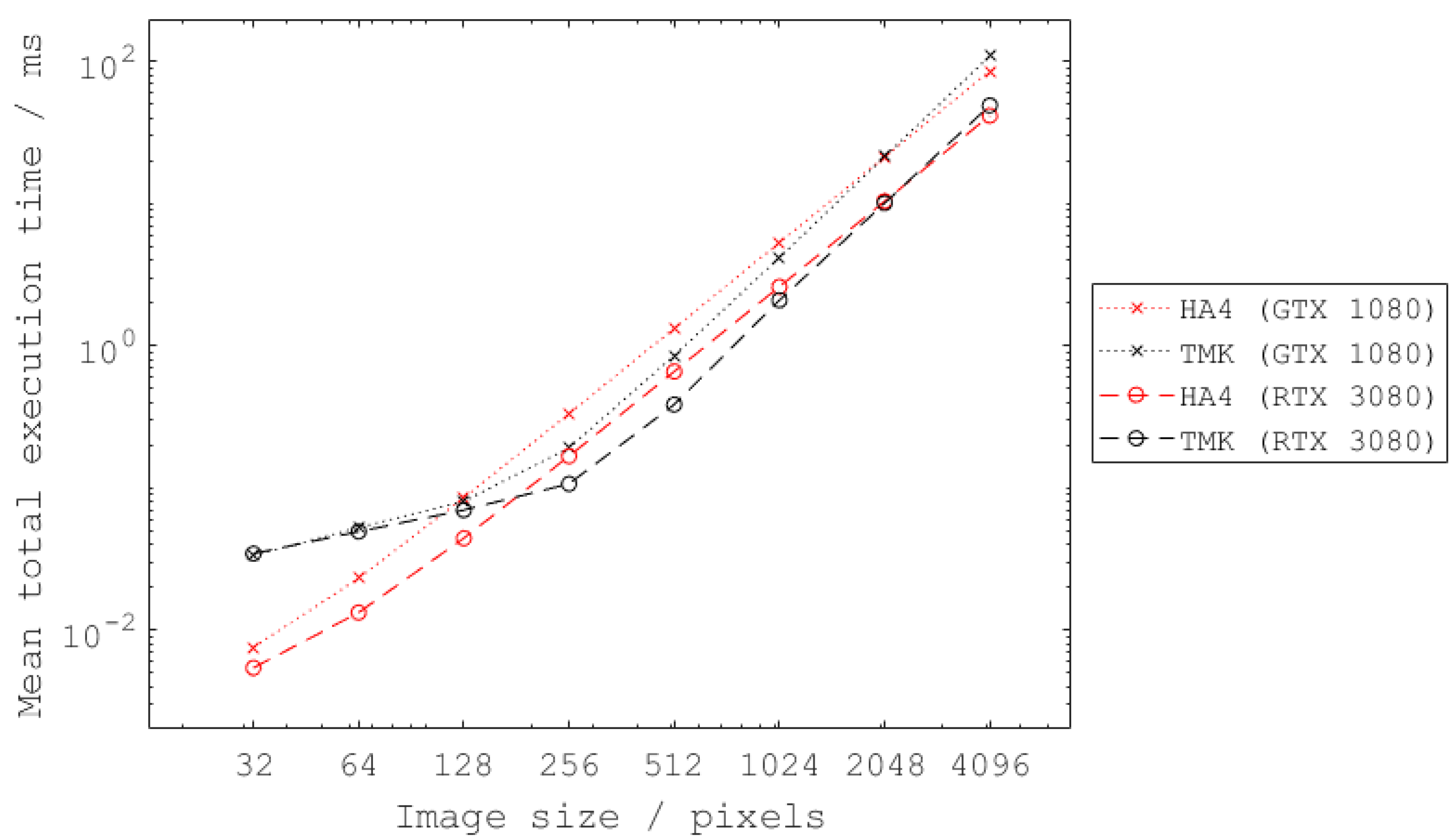
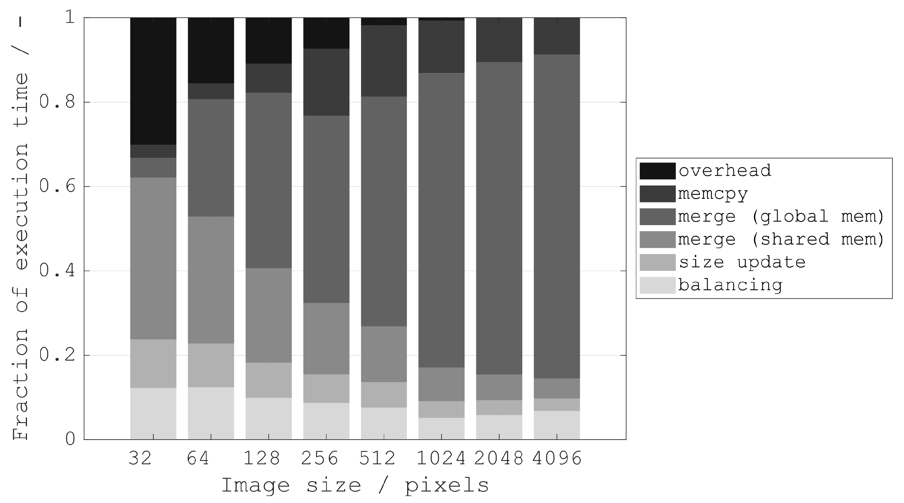
Regarding varying image sizes, the results reveal TMKs different effectiveness for small, medium and large image size. The average execution time with respect to the image size is shown in
Figure 5. The portions of total execution time for each part of TMK are shown in
Figure 6.
For small image sizes (≤128 px), the overhead for kernel launches is significant. Even though much of the tree merging is performed in shared memory, the overall computational effort outweighs the possible savings in memory transfer time.
For medium image sizes (256 px to 1024 px), the TMK performs best due an increase in possible memory transfer savings whilst processing large portions of the tree merging in shared memory.
For large image sizes (≥2048 px), much of the tree merging must be performed using global memory. This significantly slows down execution. In total, the additional computation time required for the global memory merging outweighs the increased savings in memory transfer time.
5. Discussion
Our investigations have shown that the proposed tree merge kernel (TMK) reduces overall execution times for connected component analysis when taking into account transfer times between device and host. It performs best for medium image sizes (256 px to 1024 px). For larger images, total execution time is similar to HA4 due to TMKs increasing dependency on global memory accesses. Still, required memory bandwith is drastically reduced when compared to naïvely transferring the (typically sparse) object features array from the device. This advantage is even more pronounced for images with larger granularity, i.e., less objects in total. Contrary, mere feature calculation using TMK is slower than HA4 for most cases, with noteworthy exceptions for image densities around the percolation threshold.
For future work, it may be worthwhile combining the advantages of both approaches in an algorithm which can quickly perform CCA (e.g., HA4) followed by compression of the features array before transfer to the host.
Author Contributions
Conceptualization, D.W. and C.K.; methodology, D.W. and C.K.; software, D.W. and C.K.; validation, D.W. and C.K.; formal analysis, D.W.; investigation, D.W.; resources, G.J. and A.B.; data curation, D.W.; writing—original draft preparation, D.W.; writing—review and editing, A.B. and G.J.; visualization, D.W.; supervision, A.B.; project administration, D.W. and A.B.; funding acquisition, A.B. and G.J. All authors have read and agreed to the published version of the manuscript.
Funding
This research was funded by Deutsche Forschungsgemeinschaft under grant number HA 3088/26-1.
Data Availability Statement
Publicly available software and data was analyzed in this study. The source code can be found here:
https://codebase.helmholtz.cloud/risa (accessed on 27 January 2023). The dataset used for the benchmarks (“YACCLAB”) can be found here:
https://github.com/prittt/YACCLAB (accessed on 6 October 2022). The subset “random/granularity“ was used for
Figure 4. For analysis of 256 px images, only the top-left 256 × 256 px region was used. The subset “random/classical“ was used for
Figure 5 and
Figure 6.
Conflicts of Interest
The authors declare no conflict of interest.
Abbreviations
The following abbreviations are used in this manuscript:
| CCA | Connected-Component Analysis |
| CUDA | Compute Unified Device Architecture |
| FPS | Frames Per Second |
| GPU | Grapical Processing Unit |
| HA4 | Hardware Accelerated 4-connected |
| OFS | Object Feature Struct |
| RISA | Real-time Image Stream Algorithms |
| TMK | Tree Merge Kernel |
| UFXCT | Ultrafast electron beam X-ray Computed Tomography |
References
- Nazlibilek, S.; Karacor, D.; Ercan, T.; Sazli, M.H.; Kalender, O.; Ege, Y. Automatic segmentation, counting, size determination and classification of white blood cells. Measurement 2014, 55, 58–65. [Google Scholar] [CrossRef]
- Khan, N.; Ahmed, I.; Kiran, M.; Rehman, H.; Din, S.; Paul, A.; Reddy, A.G. Automatic segmentation of liver & lesion detection using H-minima transform and connecting component labeling. Multimed. Tools Appl. 2020, 79, 8459–8481. [Google Scholar] [CrossRef]
- Rasheed, A.; Zafar, B.; Rasheed, A.; Ali, N.; Sajid, M.; Dar, S.H.; Habib, U.; Shehryar, T.; Mahmood, M.T. Fabric Defect Detection Using Computer Vision Techniques: A Comprehensive Review. Math. Probl. Eng. 2020, 2020, 8189403. [Google Scholar] [CrossRef]
- Ren, Z.; Fang, F.; Yan, N.; Wu, Y. State of the Art in Defect Detection Based on Machine Vision. Int. J. Precis. Eng. Manuf.-Green Technol. 2022, 9, 661–691. [Google Scholar] [CrossRef]
- Farhat, W.; Faiedh, H.; Souani, C.; Besbes, K. Real-time embedded system for traffic sign recognition based on ZedBoard. J. Real-Time Image Process. 2019, 16, 1813–1823. [Google Scholar] [CrossRef]
- You, S.; Bi, Q.; Ji, Y.; Liu, S.; Feng, Y.; Wu, F. Traffic Sign Detection Method Based on Improved SSD. Information 2020, 11, 475. [Google Scholar] [CrossRef]
- Fischer, F.; Hampel, U. Ultra fast electron beam X-ray computed tomography for two-phase flow measurement. Nucl. Eng. Des. 2010, 240, 2254–2259. [Google Scholar] [CrossRef]
- Frust, T.; Wagner, M.; Stephan, J.; Juckeland, G.; Bieberle, A. Rapid data processing for ultrafast X-ray computed tomography using scalable and modular CUDA based pipelines. Comput. Phys. Commun. 2017, 219, 353–360. [Google Scholar] [CrossRef]
- Windisch, D.; Kelling, J.; Juckeland, G.; Bieberle, A.; Hampel, U. Real-time Data Processing for Ultrafast X-Ray Computed Tomography using Modular CUDA based Pipelines. Trans. Inst. Meas. Control 2022. submitted. [Google Scholar]
- Windisch, D.; Bieberle, M.; Bieberle, A.; Hampel, U. Control concepts for image-based structure tracking with ultrafast electron beam X-ray tomography. Comput. Phys. Commun. 2020, 42, 691–703. [Google Scholar] [CrossRef]
- Playne, D.P.; Hawick, K. A New Algorithm for Parallel Connected-Component Labelling on GPUs. IEEE Trans. Parallel Distrib. Syst. 2018, 29, 1217–1230. [Google Scholar] [CrossRef]
- Kaever, C. Real-Time Object Recognition for Ultrafast Electron Beam X-ray Computed Tomography; Technical Report; Technische Universität Dresden: Dresden, Germany, 2021. [Google Scholar]
- Rosenfeld, A.; Pfaltz, J.L. Sequential Operations in Digital Picture Processing. J. ACM 1966, 13, 471–494. [Google Scholar] [CrossRef]
- Agrawala, A.K.; Kulkarni, A.V. A sequential approach to the extraction of shape features. Comput. Graph. Image Process. 1977, 6, 538–557. [Google Scholar] [CrossRef]
- Lacassagne, L.; Zavidovique, B. Light speed labeling: Efficient connected component labeling on RISC architectures. J. Real-Time Image Process. 2011, 6, 117–135. [Google Scholar] [CrossRef]
- Hennequin, A.; Lacassagne, L.; Cabaret, L.; Meunier, Q. A new Direct Connected Component Labeling and Analysis Algorithms for GPUs. In Proceedings of the 2018 Conference on Design and Architectures for Signal and Image Processing (DASIP), Porto, Portugal, 10–12 October 2018; pp. 76–81. [Google Scholar] [CrossRef]
- Cabaret, L.; Lacassagne, L.; Etiemble, D. Parallel Light Speed Labeling: An efficient connected component algorithm for labeling and analysis on multi-core processors. J. Real-Time Image Process. 2018, 15, 173–196. [Google Scholar] [CrossRef]
- Řiha, L.; Mareboyana, M. GPU accelerated one-pass algorithm for computing minimal rectangles of connected components. In Proceedings of the 2011 IEEE Workshop on Applications of Computer Vision (WACV), Kona, HI, USA, 5–7 January 2011; pp. 479–484. [Google Scholar] [CrossRef]
- Lemaitre, F.; Hennequin, A.; Lacassagne, L. Taming Voting Algorithms on Gpus for an Efficient Connected Component Analysis Algorithm. In Proceedings of the ICASSP 2021—2021 IEEE International Conference on Acoustics, Speech and Signal Processing (ICASSP), Toronto, ON, Canada, 6–12 June 2021; pp. 7903–7907. [Google Scholar] [CrossRef]
- Allegretti, S.; Bolelli, F.; Grana, C. Optimized Block-Based Algorithms to Label Connected Components on GPUs. IEEE Trans. Parallel Distrib. Syst. 2019, 31, 423–438. [Google Scholar] [CrossRef] [Green Version]
| Disclaimer/Publisher’s Note: The statements, opinions and data contained in all publications are solely those of the individual author(s) and contributor(s) and not of MDPI and/or the editor(s). MDPI and/or the editor(s) disclaim responsibility for any injury to people or property resulting from any ideas, methods, instructions or products referred to in the content. |
© 2023 by the authors. Licensee MDPI, Basel, Switzerland. This article is an open access article distributed under the terms and conditions of the Creative Commons Attribution (CC BY) license (https://creativecommons.org/licenses/by/4.0/).


