A Real-Time Novelty Recognition Framework Based on Machine Learning for Fault Detection

Abstract

New technologies are developed inside today’s companies with the ascent of Industry 4.0 paradigm; Artificial Intelligence applied to Predictive Maintenance is one of these, helping factories automate their systems in detecting anomalies. The deviation of statistical features from standard operating conditions computed on collected data is a common investigation technique that companies use. The information loss due to transformation from raw data to extracted features is a problem of this approach. Furthermore, a common Predictive Maintenance framework requires historical data about failures that often do not exist, neglecting the possibility of applying it. This paper uses Artificial Intelligence as Machine Learning models to recognize when something changes in the data’s behavior collected up to that moment, also helping companies to gather a preliminary dataset for future Predictive Maintenance implementation. The aim concerns a framework in which several sensors are used to collect data by adopting a sensor fusion approach. The architecture is composed of an optimized software system able to enhance the computation scalability and the response time regarding novelty detection. This article analyzes the proposed architecture, then explains a proof-of-concept development using a digital model; finally, two real cases are studied to show how the framework behaves in a real environment. The analysis done in this paper has an application-oriented approach; hence a company can directly use the framework in its systems.

1. Introduction

Since the 2010s, Artificial Intelligence (AI) and Machine Learning (ML) have become standard ways to tackle complex problems relating to Industry, Medical, Manufacturing, or Economics. Flexibility, generality, and efficiency are only some of the qualities permitted by AI to be adopted into multiple scenarios. Furthermore, academics have recently enhanced learning programs, research programs, and collaboration projects with companies to respond to the industrial world’s increasing AI and ML needs. With the upcoming Industry 5.0 paradigm, the term Predictive Maintenance (PdM) is becoming more common in the language of companies today. This type of maintenance plays an interesting role in preventing machine failures and reducing the downtime cost in a preponderant way. The cost of unplanned failure occurring in industrial machines is estimated at USD 50 billion annually as reported in the analysis by Ref. [1]. An explanation of how predictive maintenance is able to reduce the overall costs by 5–10% and the standard maintenance costs by 20–50% is reported in Ref. [2], highlighting its impact on the company’s economic aspect.

Throughout the years, the term “Maintenance” has taken different shapes and terminologies, as shown in (Figure 1) [3]:

• Reactive/Corrective Maintenance: it intervenes after a problem has occurred and is considered the oldest one;
• Aggressive Maintenance: it focuses on the performance improvement of production equipment design;
• Proactive Maintenance: it prevents machine failures and is considered to be the most used maintenance strategy today; two sub-maintenance strategies derive from this approach:

  −

  Preventive Maintenance: it is based on a periodic components’ substitution, generally the most used ones;

  −

  Predictive Maintenance: it is able to predict when a problem will occur in the future.

Since the first industrial revolution, the predictive maintenance branch has increased companies’ and scientific community’s interest in an exponential way [4]. Predictive Maintenance monitors the real status of the machine by employing events, states, and sensor data. With this kind of maintenance, component substitution is done when it is truly necessary. This approach represents the future trend of maintenance thanks to its ability to estimate when a failure will occur, reducing the cost of useless substitution and harmful downtime. Its main drawback concerns the need to collect numerous data to perform an estimation with adequate accuracy.

Often, the term “Predictive Maintenance” is used improperly by engineers, blurring it with Condition Monitoring (CM). There is a substantial difference between these two methodologies [5]: CM is based on the overcome of specific thresholds computed by a domain expert or on the datasheet basis; hence, if a warning appears, the maintainer has to intervene in solving the anomaly. With CM, there is no prediction about future issues, and an alarm is emitted when a problem has already appeared. CM is deeply explored in different application domains, as reported in Refs. [6,7,8]. The PdM’s approach is different from CM’s; using the collected data, PdM can predict when an issue will appear in the future, giving time to the maintainer to intervene before the breakdown. These two techniques are also related to two other common words: diagnostics and prognostics. Diagnostics is related to analyzing the past collected data, studying which damage occurred and the cause of that; similar to the medical environment, prognostics analyzes the data collected in the past together with the present ones to predict issues and failures in the future [9]. In detail, according to the definition of ISO 13381-1 [10], prognostics has the quirk to predict the Remaining Useful Life (RUL) of the components analyzed. Different models exist to perform a prognosis, as reported in Ref. [11], in which three different variants are well explained. Today’s PdM methodologies use more complex algorithms than the statistical ones used in the past. Among these methodologies, Machine Learning and Deep Learning (DL) cover part of today’s algorithms used to recognize anomalies and predict the Remaining Useful Life (RUL) of components analyzed. The main and common problem that companies have when working with standard algorithms concerns the complete absence of data collection about failures encountered in the past (e.g., a new machine). Hence, a standard ML algorithm cannot be applied due to the proper model training unfeasibility. This approach requires a labeled dataset that is already collected and well-known by an expert, in which each label represents the machine’s status; hence, the label gives information about the component’s RUL. When a gathered dataset does not exist (the failures labeled dataset is not present), a standard approach cannot be applied. A recent research field—called “Novelty Detection” (ND)—responds to this demand by searching for a solution to apply the PdM without a dataset collected. This paper concerns a fast and easy implementation of the Novelty Detection Framework (NDF). The paper is organized into different chapters: Section 2 presents the state-of-art and the “Related Works” about this topic; Section 3 reports the framework’s architecture with the analysis performed during the study; Section 4 concerns the Proof-of-Concept in which the framework is applied to a digital model, and at the end, two real cases are analyzed in Section 5.

2. State-of-Art and Related Works

PdM strategies used statistical parameters to study their deviation in the past, predicting when they exceeded predefined thresholds, as reported in Ref. [12]. Concerning ML, numerous algorithms could be used for this scope, from supervised, such as Refs. [13,14,15] to unsupervised, such as Ref. [16] or Ref. [17]. Generally, the Supervised/Unsupervised choice depends on how much and which type of data has been collected. In the case of a small amount of data, ML and DL are quite similar from the prediction accuracy point of view, as reported in Ref. [18]; as the number of data increases, the quality of DL prediction increases too. An example of a DL algorithm can be the Long Short-Term Memory LSTM—as reported in Ref. [19]—which requests a huge amount of data to perform PdM predicting RUL in the best way. Other examples that use DL models can be Ref. [20], where CNN is applied to a rotating machinery, or Ref. [21], where a gated recurrent unit network is applied to three different use cases. Other techniques are also used for PdM applications, such as the method used in Ref. [22] where an alternative approach performs failures identification considering the environmental noise in which a typical industrial machine is influenced (vibration due to wear or due to other vibrations coming from other machines as examples). Another approach being developed these years involves applying Reinforcement Learning algorithms to the PdM context, as reported in Ref. [23].

Most of the time, developed and known algorithms require failure data experience already collected to train a model able to recognize anomalies, as reported in the previous paragraph. Often, a common algorithm cannot be applied due to the absence of this failure collection. This paper’s idea concerns solving this problem by developing an alternative framework algorithm that does not need any past experience with failures to recognize anomalies or problems. The technique is also known as Novelty Detection, a parallel branch of Predictive Maintenance that can predict failures and changes without a dataset already collected. ND can be applied in different situations depending on the data pattern collected; it can be recognized in three main contexts [24]:

• Point pattern: where individual instances are different compared to the trained ones;
• Collective pattern: in which a small sub-dataset is a novelty concerning the whole distribution;
• Contextual pattern: in which novelty can happen within a specific context.

This paper concerns Contextual Pattern recognition; hence, the framework recognizes a change in the data due to some external events (environment, maintenance operation). Novelty detection has been developed in the scientific community thanks to its ability to satisfy company requirements. Papers such as Refs. [5], [17], or [25] have worked on this topic, framing this as a new research field to help companies implement a preliminary framework to collect data until a real PdM infrastructure is built. This detection type can be applied in numerous domains such as medical, robotic/industrial, vision surveillance, and other fields, as reported in Ref. [26] that deeply analyze this research topic.

A common Novelty Detection algorithm often uses complex algorithms to perform its tasks, but sometimes, highly skilled systems are unavailable (e.g., embedded systems). The work developed in this paper wants to give an alternative use of ML that differs from a common utilization, able to perform novelty recognition in real-time, requiring very few computational efforts. Easy mathematical computations allow us to use an embedded device as a framework’s container, which is not common in the known approaches. The alternative approach is based on a real-time ML error computation between predicted and real data to understand if the incoming information is similar to the trained ones; in case of deviations, a domain expert understands if the system’s status is healthy or faulty. This technique can be used without statistical features but with proper raw data preprocessing, as reported in the “Architecture paragraph” below. A comparison between known algorithms and the one used in this paper can be resumed in the following clear steps:

• Low computational effort required: thanks to easy mathematical computations and the models selected, this algorithm requires low energy in terms of computational effort;
• Real-time: thanks to the low computational effort, the system can work in real-time as reported in the “Discussion paragraph” in which the resume table reports the small time required for each framework’s stage;
• Flexibility and scalability: the framework has a general template in which different sensors can collect data to understand if some of them are changing from the trained one. The sensor adding is always possible without changing anything in the framework but just retraining/updating the model with new data added (as explained in the following paragraph);
• Data collection: using this framework, healthy and faulty collection can be collected in order to build a complete dataset for a future PdM implementation.

3. Proposed Predictive Maintenance Architecture

The architecture proposed in this paper concerns a “Novelty Detection Framework” (NDF). The system is divided into modules responsible for performing different tasks (Figure 2). Every framework’s unit in this chapter is explained in detail to understand how it works.

3.1. Maintained System

The elements of this section interconnect the machine’s parts under study with the software framework. This module can be composed of sensors, cameras, machine logs, and every element can help the data collection phase. As mentioned, this framework’s essence is based on comparing the initial trained data to the actual ones to recognize if some difference appears in the data pattern. In a real environment, two possible situations can be found:

• A system that always works in the same condition with the same parameters, such as a drilling machine’s asynchronous motor or an injection molding machine’s motor;
• A system in which the condition often changes, such as in car engines or linear motors in which the speed and parameters can change at every time instant.

In the latter case, the conditions must lead to the same type to obtain a reference in which a training process is consistent (an example can be the same motion of a linear motor always with the same parameters). This unit is also responsible for performing another important operation—the data sizing; every data collected by sensors must always be of the same size to perform the prediction in the best way. In this paper, the word “Dataset” will refer to a record with a number of samples that is always equal.

3.2. Data Source Unit

This section is responsible for storing data on a database installed locally or in a remote cloud. Every dataset uploaded to the database contains a specific format useful for the framework; indeed, it is possible to imagine a sort of table in which every row represents a single database record while the columns represent all the features used to characterize a data pattern (such as temperature, acceleration, or sound). Data is labeled in every column with the name of that specific feature, as reported in the following

Table 1. Data labeling.

id	Timestamp	Fs	Acc_1	Acc_2	…	Acc_n	Sound_1	…	Sound_n
…	…	…	…	…	…	…	…	…	…

:

Hence, more columns are present in the data frame used depending on the time and the sampling frequency.

3.3. AI Unit

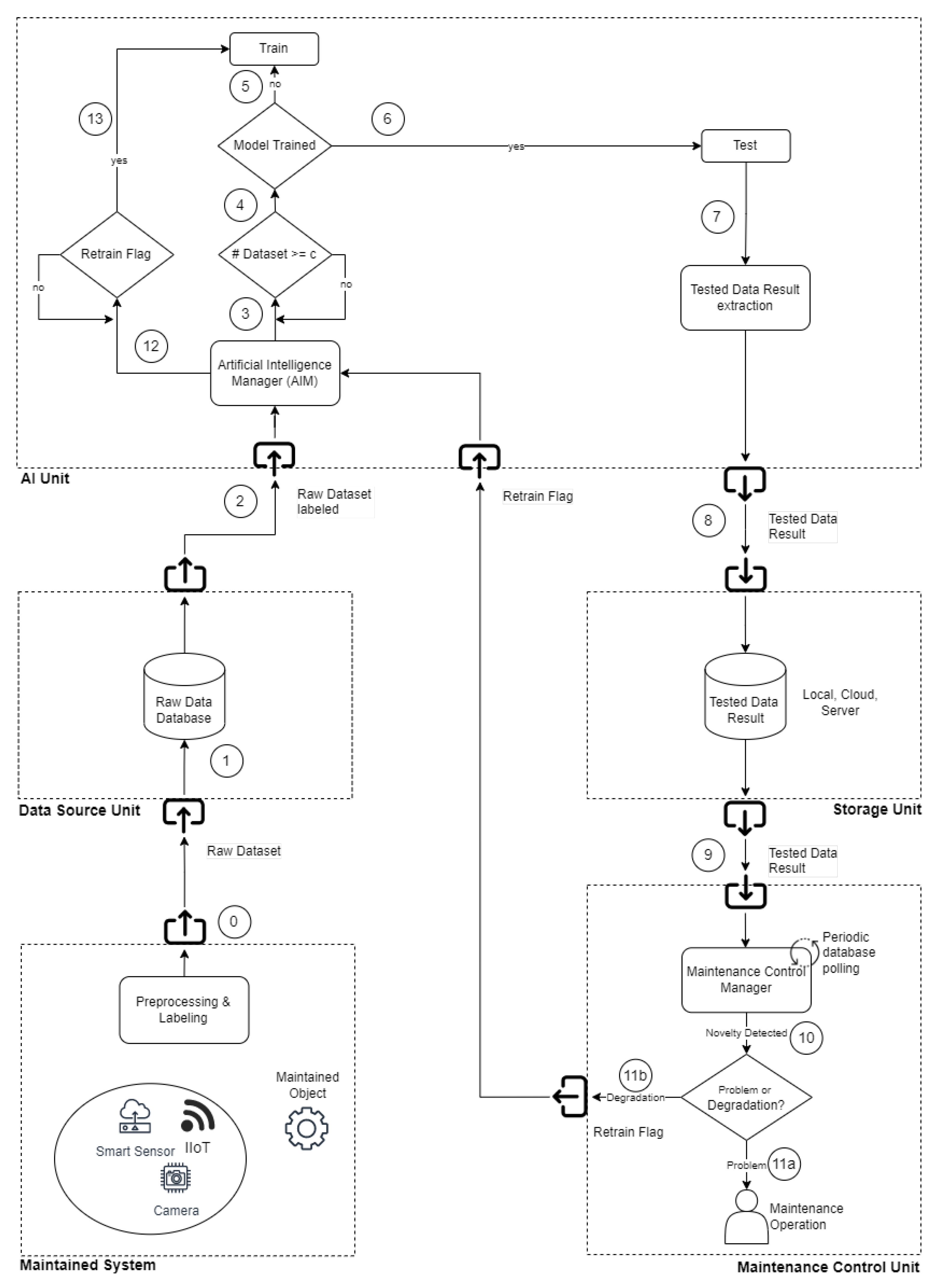
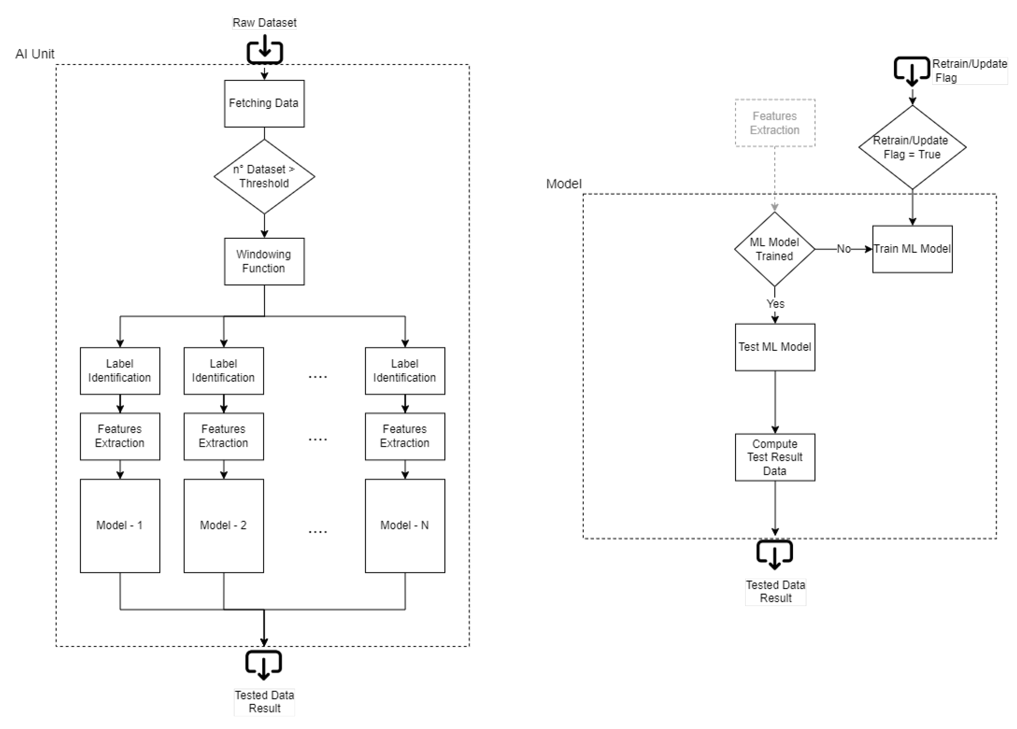
The AI Unit is shown in Figure 3, the framework’s “brain”. As a standard ML approach, the parts that compose the process flow are represented in Figure 4:

As mentioned before, the idea of this paper is to give a different use of ML compared to a normal flow. A common approach follows the standard way that a dataset is divided into Training Set, Testing Set, and Validation Set; in this case, the framework continuously works in testing mode to compute the prediction error for every dataset that arrives in the database. Monitoring this error makes it possible to understand if a deviation occurs in the collected dataset. Every time that data collected are similar to the ones used for Training, the error obtained is low. In contrast, if an issue happens in the machine, the error tends to increase due to different behavior in the data pattern collected. This type of detection does not predict only problems; it can also understand when a novelty related to a change appears in the dataset (typical in a real situation, an example can be environmental changes).

For this reason, the trained dataset must represent the whole machine’s behavior. The number of datasets chosen for the training depends on the framework’s application: by increasing the number of training datasets, the prediction’s accuracy increases too (the risk of a false positive due to a change is low); however, training the framework with a small number of datasets allows using it earlier, but the maintainer may work more during the first days by updating it (the risk of detecting a change is higher). A trade-off concerning the duration of the training process has to be defined. Generally, companies that design machines/components always have a period in which the machine/component is calibrated and tested; this period can last from a few days to an entire month, and it could be useful for the training process. An entire environmental changes cycle (such as the morning, the afternoon, and the night) can be useful for gathering all the possible components’ changes. Sometimes the data collected can change over the day: during the morning, when the temperature is low, the machine has a certain accuracy that changes during the afternoon due to the higher temperature reached. There is no general rule explaining how many datasets are gathered; a possible hint is to collect one week’s worth of data to record a consistent dataset. The best situation in which this framework can be trained is at the beginning of the machine’s life (e.g., after the assembly process). Nevertheless, the framework can also be trained after years of machine work; in this case, the framework performs the training at that moment and cannot recognize preexisting faults due to the absence of healthy datasets. However, the nature of failures leads to a machine’s worsening over time, detecting them also if training is performed with a partially faulty system; hence, thanks to the system’s adaptability, the absence of a healthy dataset is not a problem, but it may afflict the framework’s accuracy. The first stage of the ML process flow is preprocessing, which consists in taking every single dataset from the database and recognizing which kind of features are stored (such as Acceleration, Sound, or Temperature). Then the AI manager applies a windowing function for each type of feature recognized: the windowing approach divides the large dataset’s features into a parametrized small number of windows (for example, acceleration is divided into $k_1$ windows, sound into $k_2$ windows) depending on the resolution wanted in the framework recognition: a higher number of windows corresponds to a higher prediction’s resolution; on the other hand, the system works more complexly due to the higher number of windows to predict. 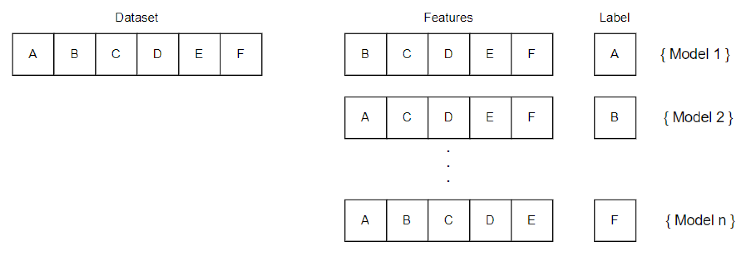Each window is associated with a predictor (AIUP), which uses $i_{th}$ window as a label and the others as features (Figure 5). Thanks to the windowing approach, each window is used to perform computation by condensing the initial amount of data (a cumulative sum is used for each window in this paper). The mathematical representation of the windowing function and cumulative absolute sum for each window is reported below:

$$[x_1,x_2,\dots ,x_n]->\left\{\begin{array}{c}[x_1,x_2,\dots x_m]withm<n\hfill \\ [x_{m+1},x_{m+2},\dots x_{m+k}]withm<m+k<n\hfill \\ \dots \hfill \\ [x_{m+k+1},x_{m+k+2},\dots x_n]\hfill \end{array}\right.$$

While the cumulative absolute sum function used is the following:

$$\left\{\begin{array}{c}[x_1,x_2,\dots x_m]\hfill \\ [x_{m+1},x_{m+2},\dots x_{m+k}]\hfill \\ \dots \hfill \\ [x_{m+k+1},x_{m+k+2},\dots x_n]\hfill \end{array}\right.->\left\{\begin{array}{c}\sum _{i=1}^m\left|x_i\right|\hfill \\ \sum _{i=m+1}^{m+k}\left|x_i\right|\hfill \\ \dots \hfill \\ \sum _{i=m+k+1}^n\left|x_i\right|\hfill \end{array}\right.$$

The feature extraction and labeling phase follow the preprocessing stage. This block is responsible for preparing data for the following ML model training. With a multi-threading approach, a feature is extracted from the dataset by converting it to a label; this procedure is done for each window/feature, creating a number of labels equal to the number of windows and predictors. This rule is schematized in the following figure:

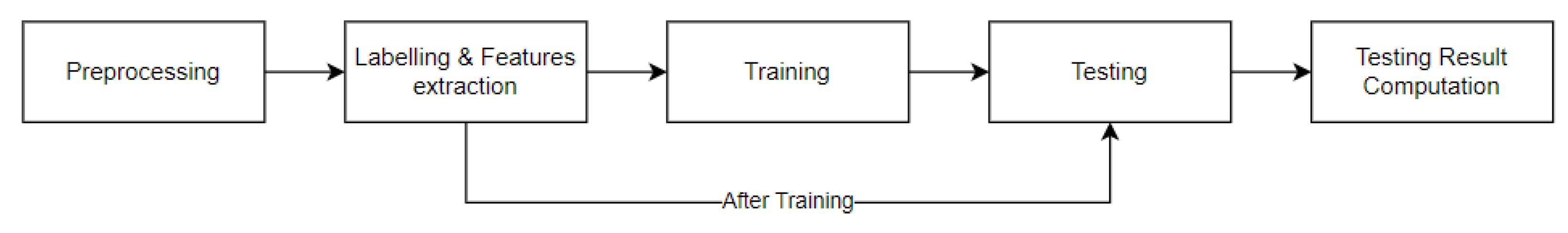
At the end of the preprocessing stage, a number of trainsets equal to the number of windows are created; each trainset is used for the related ML model training. Then, the testing phase follows the training one. The same preprocessing approach is applied to each new dataset; in the end, the label related to $i_{th}$ model is predicted and compared with the real one, computing the error used for novelty detection. Hence, the AI Unit can be divided into two different macro-stages:

• The first part is related to the training process in which the system waits for a predefined number of data to train the models;
• The second part is the testing process in which incoming data are continuously tested to compute the predictions’ error results.

For the Training phase, three regressors are tested to visualize the potential differences in the prediction behavior. The models used during the evaluation are:

• Linear Regressor;
• Decision Tree Regressor;
• Random Forest Regressor.

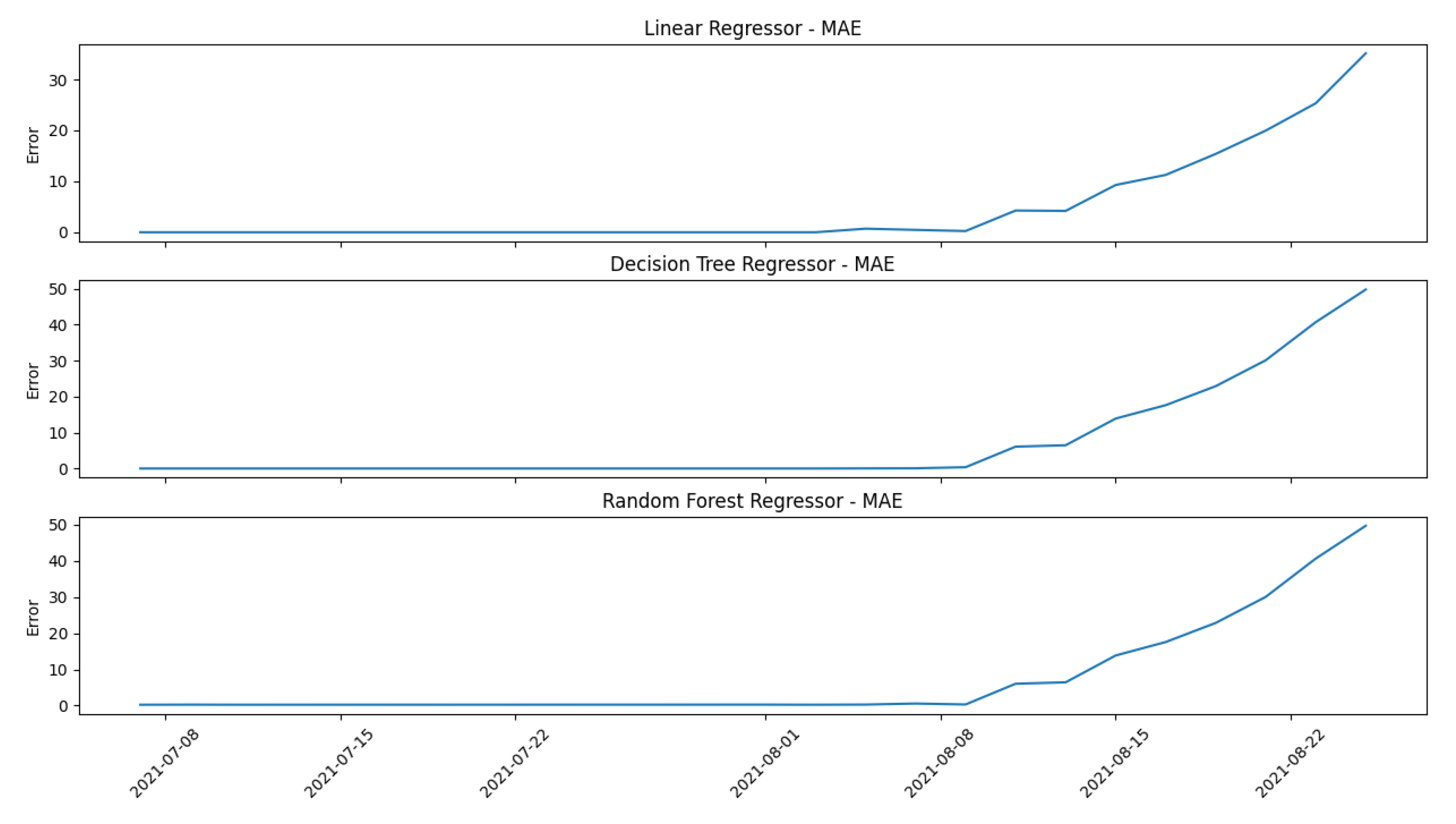
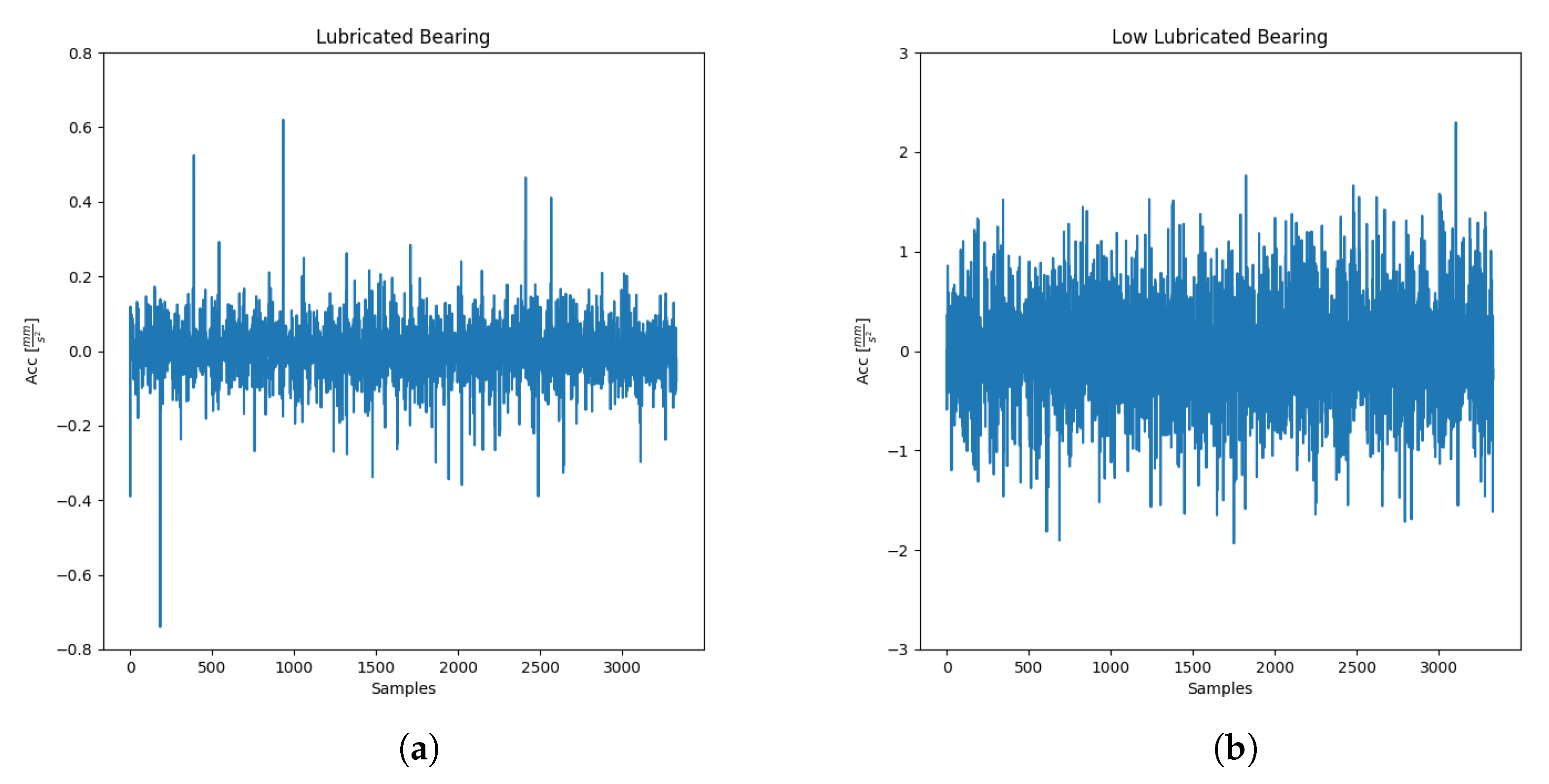
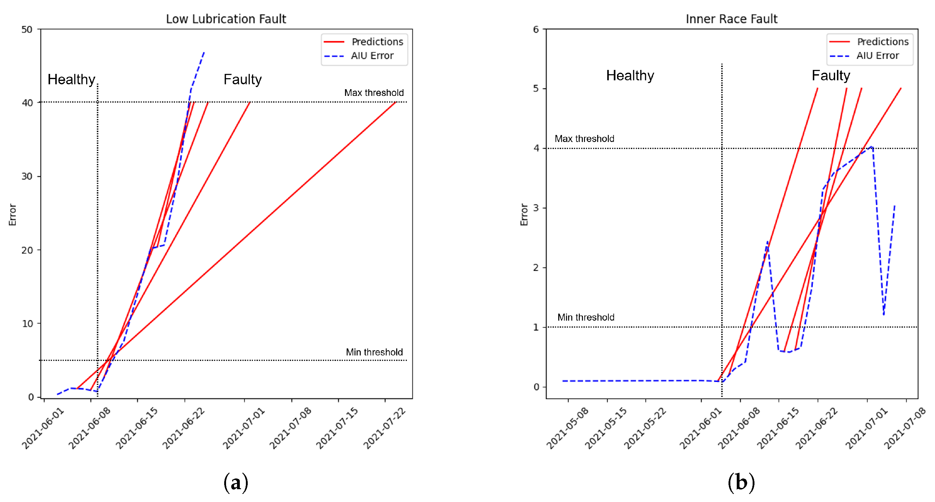
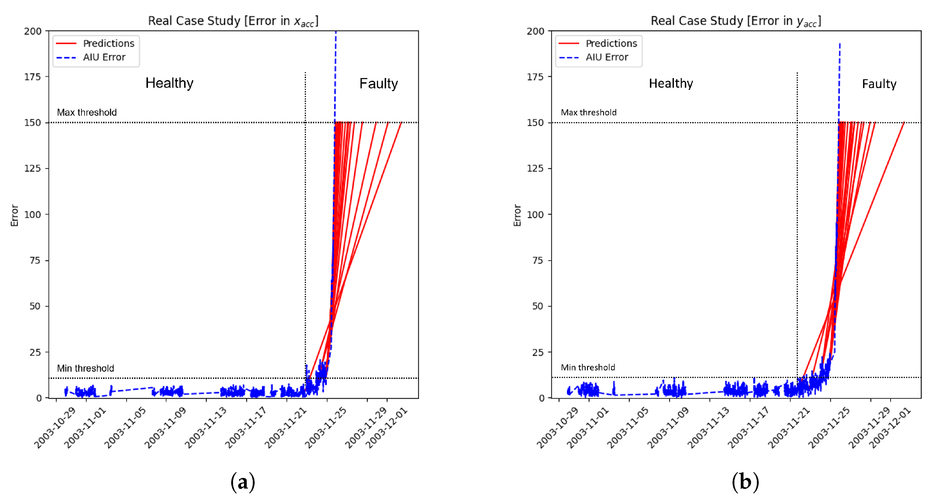
The “Low Lubrication Case” of the “Digital Model” (better explained in the following paragraph) is used as a representative example to see how the mentioned models work in order to compare them. Generally, a system works always in the same way: at the beginning of life, when it is healthy, the error computed by the model’s prediction is low; when the failure appears, the error’s prediction starts to increase. A further confirmation that a general system works in this manner is shown in Section 5 in which the real cases behave exactly like the digital model used for the proof-of-concept, starting with a low error that increases at the end of the life when the failure appears. This general behavior is shown in Figure 6 and Figure 7: the former concerns the models’ selection, while the latter represents the errors’ selection.

The results obtained by comparing the three models are almost identical. In the Linear Regressor model, the y-scale has a lower variance in terms of the range in which the error can span, while in the other two models, the y-scale range is almost the same. The user can choose one of the three models with no particular weakness; generally, the tree models have better accuracy than the easier Linear Regressor, but this one has the advantage of being faster when the training process is performed. Decision Tree Regressor and Random Forest Regressor work similarly from a general point of view: the former works only with decisions while the latter works with decision trees. The main difference between them concerns the accuracy obtained and the computation’s complexity: a Decision Tree Regressor has lower computational complexity and accuracy than a Random Forest Regressor. The operator can choose one of the three models depending on the application in which the framework operates: for example, if there are no “computational effort thresholds”, such as a workstation or a computer, a Random Forest Regressor can be used to obtain an accurate prediction, while if the aim is to deploy the framework in a stand-alone embedded device, a Linear Regressor or a Decision Tree Regressor can be used in order to reduce the overall computational effort. The paper’s framework is uploaded in a workstation to compute the predictions and results; hence, a Random Forest Regressor is chosen as the reference model.

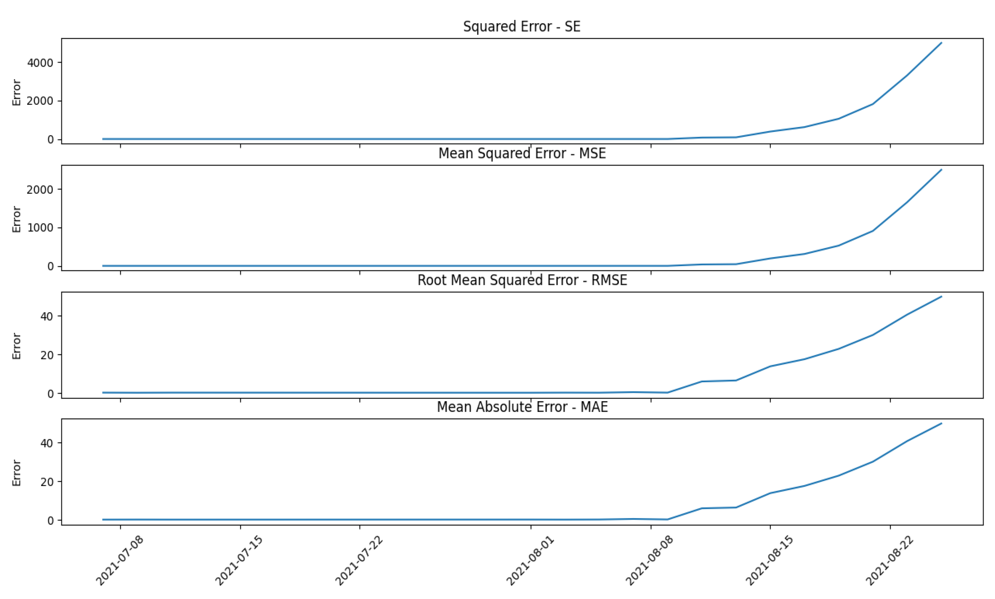
Furthermore, different errors were also evaluated during the study: Squared Error (SE), Mean Squared Error (MSE), Root Mean Squared Error (RMSE), and Mean Absolute Error (MAE), with the shape reported below:

$$SE(y,\widehat{y})={\sum }_{i=0}^{n-1}{(y_i-\widehat{y_i})}^2$$

$$MSE(y,\widehat{y})=\frac{1}{n}{\sum }_{i=0}^{n-1}{(y_i-\widehat{y_i})}^2$$

$$RMSE(y,\widehat{y})=\sqrt{\frac{1}{n}{\sum }_{i=0}^{n-1}{(y_i-\widehat{y_i})}^2}$$

$$MAE(y,\widehat{y})=\frac{1}{n}{\sum }_{i=0}^{n-1}|y_i-\widehat{y_i}|$$

where $y_i$ is the real value while $\widehat{y_i}$ is the predicted one. Figure 7 shows different error pictures computed on the same predictor using a Random Forest Regressor (RFR).

As shown in Figure 7 there is a substantial difference between the obtained results; the last two graphs are more disrupted than the first two because they follow the prediction’s behavior faster. As in the AI model selection case, there is no particular rule for the error model selection. A possible solution could be to configure all four error models to monitor the deviation by creating dedicated predictor agents to perform the computation, but this creates waste from a computational energy point of view. The latter two error models show very similar behavior because of the huge likeness in the formula behind them; with the same number of samples, the MAE has $1/n$ while RMSE has $\sqrt{1/n}$, multiply the square root member. The similarity in the graphs above is due to the number of data used for the computation: when the number is low, the $1/n$ and $\sqrt{1/n}$ are very comparable, also bringing a similarity in the results obtained. In this case, the operator can again choose which error model or which error models the framework has to use to monitor the behavior of the machine. In this paper and the following case studies, the error chosen for the evaluation is the MAE. 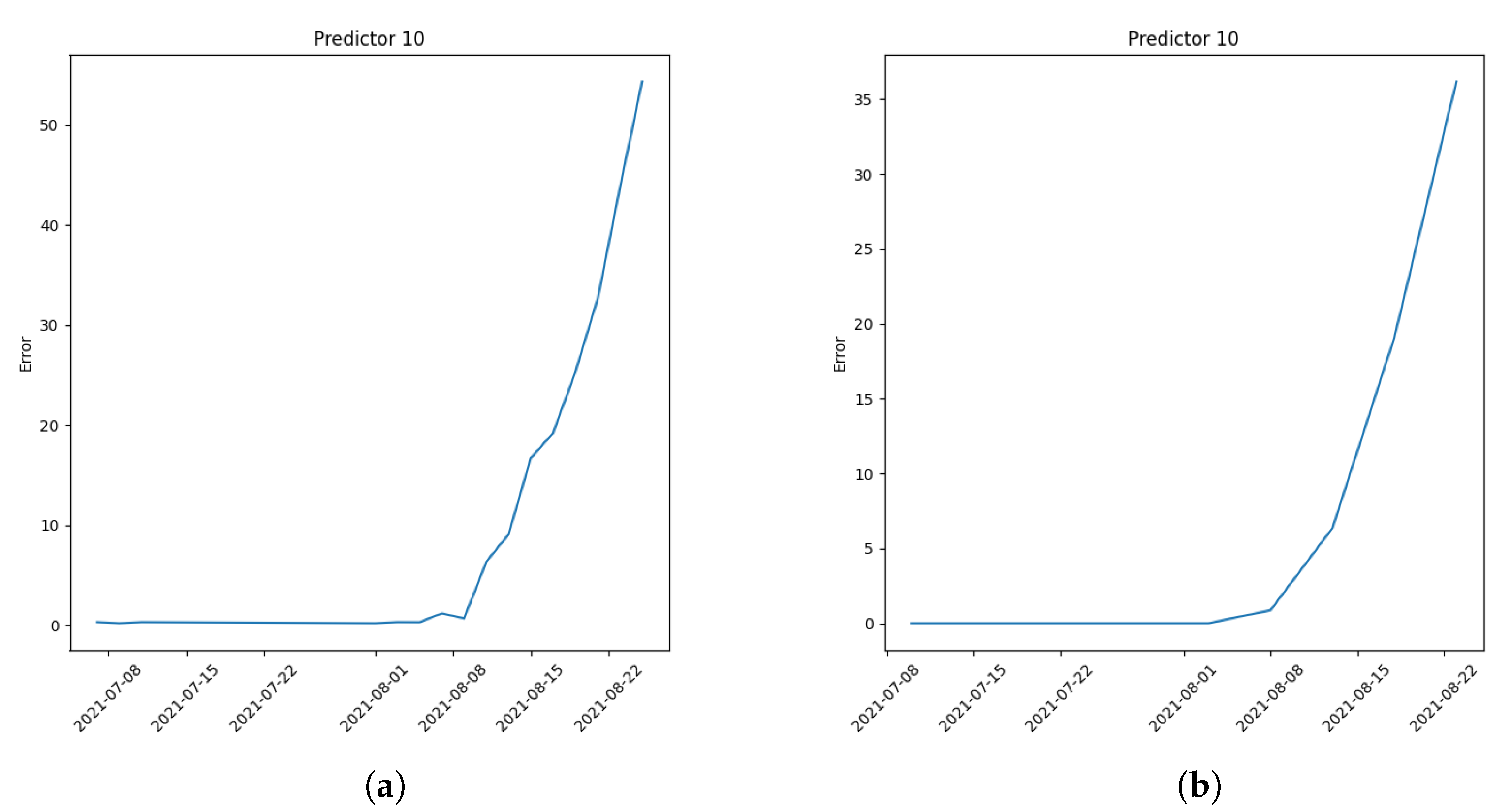Figure 8a,b show two examples in which the error is computed with two sample ranges n; Figure 8a shows the last two records while Figure 8b shows the last five records:

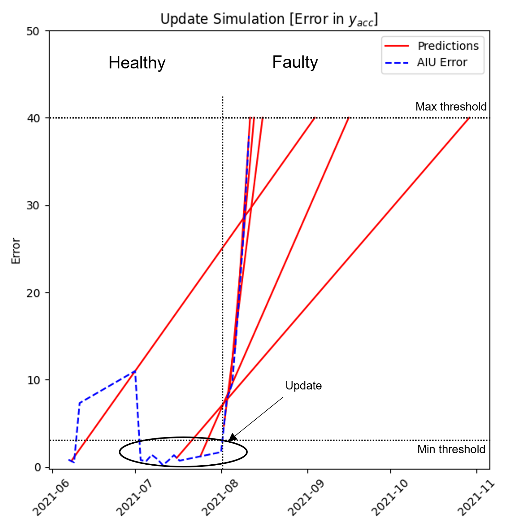
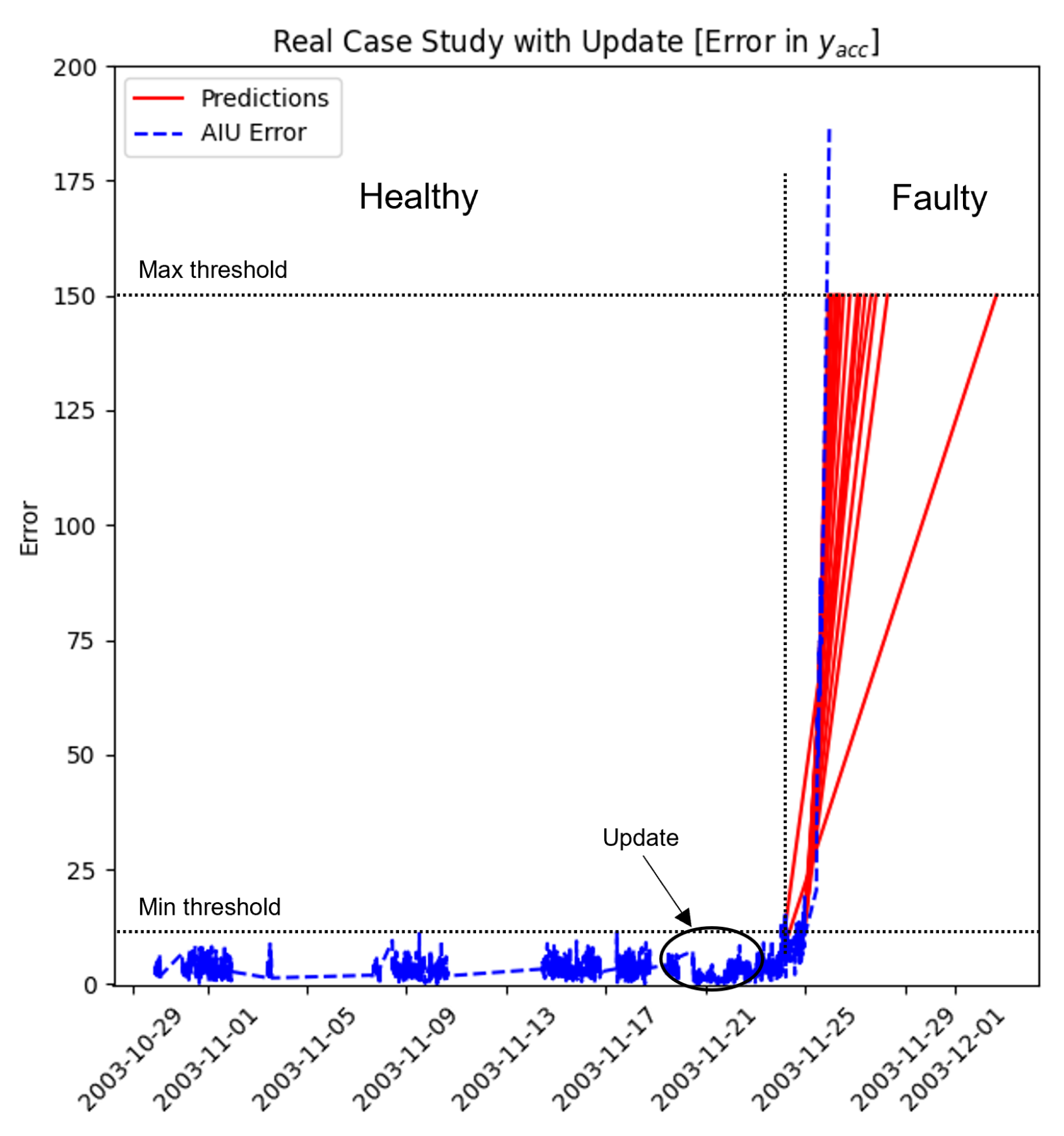
A two-sample error is chosen for the following experimental executions because of its ability to predict quickly. Another ability of the main framework concerns the possibility of updating or retraining the already trained models: as explained above, Novelty Detection can understand when something new happens in the system; this change can be related to an issue or a change does not create any problem. For this reason, when a novelty appears, the maintainer has to examine if the problem truly exists in order to choose one of the following procedures:

• Models Update: in the case in which the data collected are different from the trained ones, but this change is not related to an issue in the machine, the maintainer can update the framework with the last parametrized n data, considering the incoming data as good ones. Thanks to the models’ update, a substantial reduction of the error value is performed;
• Models Retrain: when a problem or a component substitution is performed in the machine, the retraining process is necessary due to the inevitable data change in the prediction (a common change could be a shift error in the data collected). The maintainer can decide to retrain the models by neglecting all previous ones and returning to the beginning phase.

An example of the update/retrain function is shown in the following “Digital Model” paragraph. The model update function also collects consistent datasets of the component under study to help the beginning data collection, which is useful to create the machine’s behavior history for future PdM implementation.

Recapping the AI Unit’s phases (Figure 3):

• Data Fetching Phase: in a continuous loop, the Unit waits for new data uploaded in the local/remote database to take them for the following Training or Testing phase;
• Training Phase: when a predefined number of datasets are uploaded to the database (depending on how long the train dataset collection lasts), the framework understands that the training process can start. After the Training process, several models are created as a function of the features extracted (hence depending on the number of windows of the windowing function);
• Testing Phase: after the training phase, every dataset uploaded is processed by the framework with a number of predictors equal to the number of models previously created. Then, every predictor estimates its label with an error; the upcoming failures conduct the dataset to change its shape, increasing the error in the prediction. The number of predictors equal to the number of features can help in error recognition by covering all the data distribution.
• Retraining/Updating Phase: in some cases, the model error deviates without a real problem on the machine; in this case, the maintainer can update the models trained, considering incoming new data as “normal”, resetting the error value. The retraining process is necessary when a maintenance operation is performed; then, past data are neglected, and only new data are used for future predictions.

3.4. Storage Unit

After the elaboration done by the AI Unit, the results obtained are stored again in a database; this way, it is always possible to see the history of data collected till that moment.

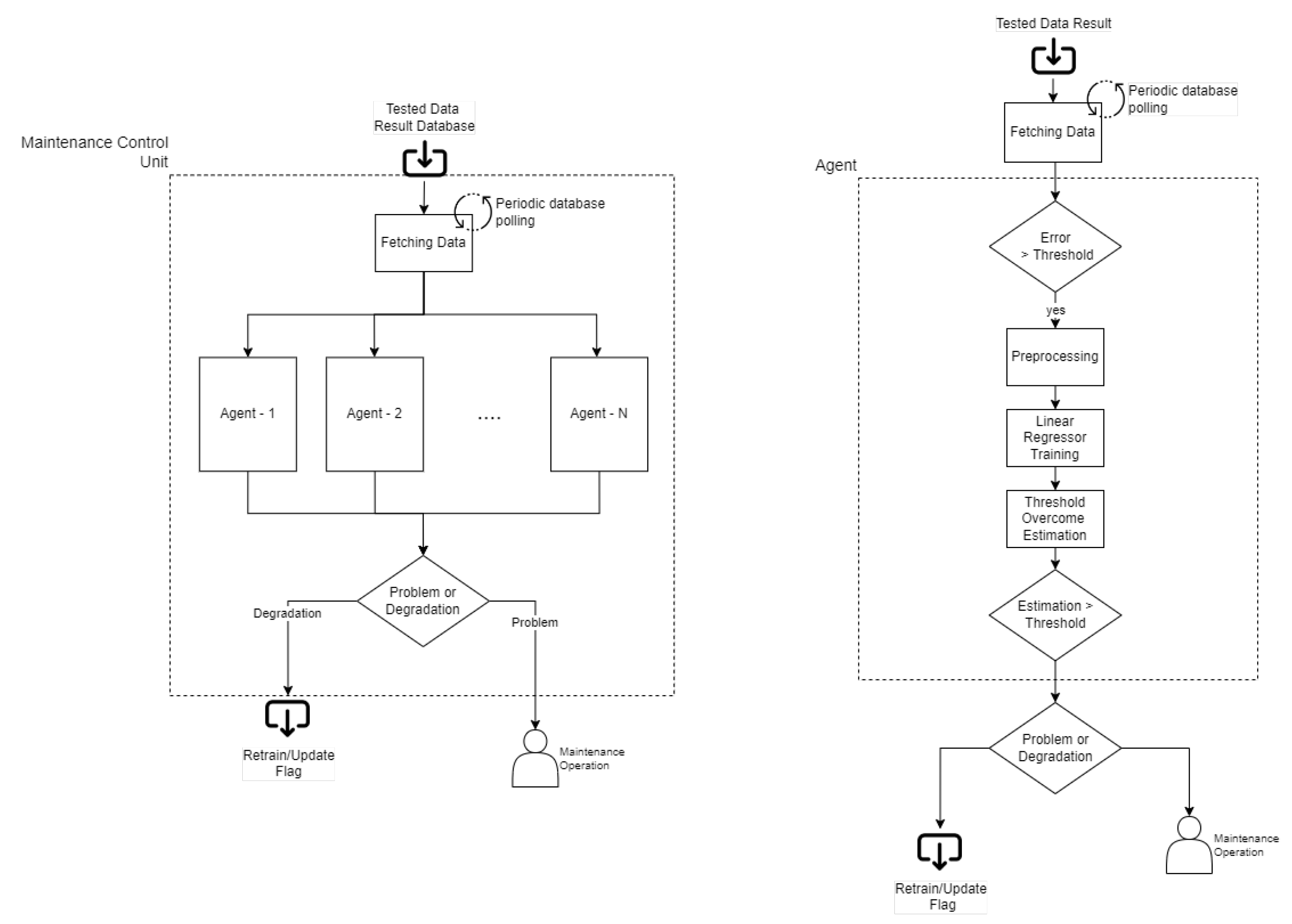
3.5. Maintenance Control Unit

The Maintenance Control Unit (MCU) is developed as a software Multi-Agent System (MAS), composed of a system and an application level. This section analyzes the MCU system and application levels from an architectural, functional, and procedural point of view by entering into its implementation details.

As presented, NDF measures the evolution over time of a system using a set of metrics and predicts the time in which these measures become relevant to detect system model changes. As explained above, two main modules can be identified in the NDF environment: AIU and MCU. AIU computes raw data and provides information about model accuracy over time using prediction error. MCU monitors this model’s accuracy degradation over time to detect relevant changes in system behavior compared to the trained ones. Hence, MCU performs:

• Sensing error over time, produced by AIUPs;
• Evaluating current AIUPs’ errors by applying a set of condition-action rules;
• Performing time predictions of AIUPs’ errors degradation through their most recent data result;
• Producing maintenance events to notify AIUPs’ models changes.

AIU consumes raw data from a system and provides different error data types. MCU processes these results to detect changes, making the Remaining Time to Retrain (RTR) predictions. RTR is similar to RUL in a PdM environment; however, it is related to a different type of prediction: in RUL, the prediction concerns the computation of the remaining time before the occurrence of a failure; on the other end, RTR concerns the computation of the remaining time before exceeding a threshold defined as a warning value.

MCU performs its task by separately analyzing all errors collected by AIU. Since the results collected are related to different AIUPs, MCU can be divided into smaller independent units (agents), and each of them computes a result for a fixed model (AIUP) (Figure 9). For this reason, MCU is developed as a software MAS.

Two main “actors” can be identified in the architecture’s MAS:

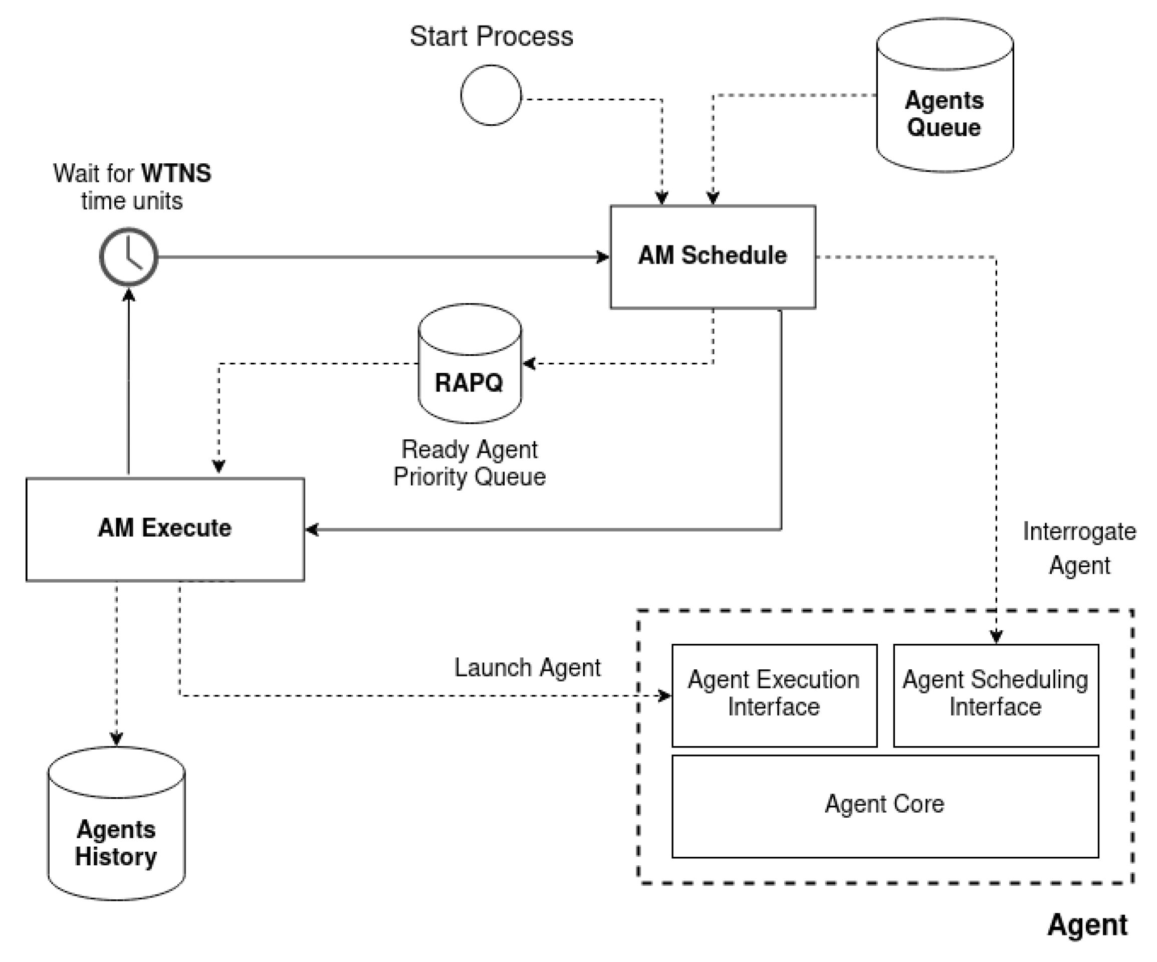
• Agent Manager (AM) detains control flow of the system process and manages the life cycle of single agents. It is responsible for maintaining, scheduling, and executing each agent over time;
• Agents interfaced with the Agent Manager: they solve their designed job by executing their Agent Program (AP) into the system process. Each agent holds its intelligence internally in terms of capabilities and features.

Generally, AM acts as a dummy entity, and the whole complexity of the system is moved onto the agents. Furthermore, a secondary actor appears in the MCU, the Agent System (AS). AS controls AM and is responsible for initializing and configuring agents, launching AM execution, and waiting into sleep mode until AM execution ends or an AM exception occurs.

AM is implemented in the MCU system control layer and is not involved in the MCU application process. During AS initialization, the AM and all agents are loaded. Until AS launches AM, the AM main process will start, and AS will go idle. As shown in Figure 10 the AM main process comprises a stoppable loop of three sequential phases identified as agents scheduling, executing, and waiting for the next scheduling. During agents scheduling, AM collects ready agents and computes the Wait Time for the Next Scheduling (WTNS). During agents execution, AM executes the collected ready agents. To increase MCU’s reliability, the AM will wait for a Maximum Wait Time for Execution (MWTE). Finally, AM will sleep for WTNS time units before the next scheduling.

Model Change Detector Agent (MCDA) architecture is developed as an agent that perceives the environment and its state, applies some condition-action rules, and executes a given action. Each agent executes its program by performing the following operations:

• Sense environment and obtains k errors back in time, related to a given AIUPs’.
• Applies a condition-action-based rule to evaluate the last error value and detect model changes. The agent works in a specific operative range composed of low and high thresholds (lowest and highest bounds). The lowest bound represents when the agent starts its prediction, while the highest bound represents the maximum error allowed. This last value is used for the RTR prediction;
• Performs an “Average” computation of the parametrized k errors selected back in time; when the lowest bound is overcome, the system triggers the related software agent that takes the last k errors back in time, dividing this errors-set into two different parts, an “oldest” and a “newest” part; at the end, an error and time average are computed for both the first and the second part selected, obtaining two points useful for the following trend identification phase;
• Performs the trend degradation analysis by training a Linear Regressor (LR) on the two points computed in the phase before and making a prediction on the time of reaching a certain error value;
• Apply a condition-action-based rule on the predicted time to degradation value to decide whether the model changes. The notification is performed if the predicted time is closer to a parametrized notification prevention tolerance time. Otherwise, the agent program ends. This approach avoids notifying model changes, which error threshold value will most likely be reached in a long time;
• Notify model change for a given predictor and error type. The notification is performed thanks to the interface actuation function that permits emitting a notification with a related message. The notification message contains the detected predictor that changes with the time prediction of reaching the error threshold value.

The MCU application architecture is composed of different MCDAs that operate independently over time. Each MCDA executes its AP periodically.

To summarize, MCU is implemented as a leader-follow, time-triggered agent system. Both system and application architecture are entirely developed using multi-threading and Object Oriented Programming approaches. Additionally, inheritance and polymorphism are used to develop the hereditary hierarchy of agents. Thanks to its code reusability optimization and extendability, this MAS allows the development of new applications easily through new agents.

The framework’s code will be available at the following link: https://github.com/PIC4SeR/PdM_NoveltyDetectionFramework.git (accessed on 1 November 2022).

4. Proof of Concept—Digital Model

For the proof-of-concept and validation of the whole framework, a multibody digital model is developed using Simulink’s toolbox to generate datasets for training and testing. The model developed consists of a rotating shaft with two bearings at the extremities and a gear in the middle dedicated to the torque transmission. The aim concerns the design of a complete digital model that simulates failures to test the framework’s response and prediction ability. In Figure 11, the digital model designed is shown:

The digital model is voluntarily simplified because the aim concerns understanding how NDF works during a change in the data pattern. A realistic mechanical model runs away from this paper. The vibration propagation is a fundamental property that the model must possess; this property allows sensing vibrations from other components far from the noise source (an example can be a vibration felt by the right bearing with the left bearing subjected to the noise source). For this scope, “virtual accelerometers” are used to understand how vibrations affect the shaft and bearings to recognize failure conditions or problems during the rotation. The material used for all the components is the same, which is steel with the following properties (

Table 2. Material Configuration.

Density	7500 kg/m${}^3$
Young’s Modulus	210 GPa
Poisson’s Ratio	0.30

):

In the following sections, each component is analyzed in further detail.

4.1. Shaft

The shaft is divided into different components representing each section diameter change; hence, a rigid connection is used to link all the “fragments” together, assembling the whole shaft. A discretization of two finite elements reduces the model simulation complexity. The gear affects the shaft with a radial force and a torque; bearings are responsible for the noise generation represented by a random uniform force impulse, which affects radial x and y directions.

4.2. Bearings

Each bearing is divided into two parts: an internal ring linked to the shaft by means of a rigid joint and an outer ring rigidly connected to the fixed reference frame of the “environment”. The representation of the roller vibration is performed using a planar joint with three degrees of freedom (dof) that gives the possibility to move in x and y directions but also around z with predefined stiffness and damping values. Hence, x and y directions represent the vibration directions generated by each sphere during rotation designed as small impulses acting on the inner ring; the motion around z represents the rotational viscous damping due to the bearing’s lubricant. The remaining dof are neglected to simplify the computations done by the simulator.

4.3. Simulations

Numerous simulations are performed to represent different fault cases. The chosen tests performed on the framework are the following:

• Low Lubrication: a lubrication degradation condition is simulated inside bearings. This situation is represented by increasing the variance range of the impulse’s force acting on the shaft. Two accelerometers are placed on the bearings and on the shaft to measure vibrations emitted and transmitted. Hence, in every simulation, the accelerometers measure an increase in general noise with a reduction of rotational viscous damping around z. The parameters change in each simulation in the same manner for the left and the right bearing. It can imagine that every simulation has different time instants in which a maintainer takes data from the machine to monitor; for this reason, each simulation is delayed by one day. This case is represented in Figure 12a,b in which the lubricated and not completely lubricated bearings are shown. The vibrations shown are measured on the right bearing:
• Inner Race Faults: as reported in Ref. [27], a general rolling bearing has four standard types of fault that can occur over time; these faults are “translated” as frequencies with the following names and shapes:

  −

  Ballpass frequency outer race (BPFO), a fail occurs in the bearing’s outer race:

  $$BPFO=\frac{n{f}_r}{2}(1-\frac{d}{D}cos\varphi )$$

  −

  Ballpass frequency inner race (BPFI): a fail occurs in the bearing’s inner race:

  $$BPFI=\frac{n{f}_r}{2}(1+\frac{d}{D}cos\varphi )$$

  −

  Fundamental train frequency (FTF): a fail occurs in the bearing’s cage:

  $$FTF=\frac{f_r}{2}(1-\frac{d}{D}cos\varphi )$$

  −

  Ball spin frequency (BSF): a fail occurs in the bearing’s rolling elements:

  $$BSF=\frac{D}{2d}(1-{\left(\frac{d}{D}cos\varphi \right)}^2)$$

  where $f_r$ is the shaft speed, n is the number of spheres, $\varphi$ is the angle of the load with respect to the radial plane, d is the sphere diameter, and D is the bearing’s radius between two rings.
  For the proof-of-concept of this paper and to test the framework in different situations, an Inner Race Fault is simulated, as shown in Figure 13a,b. Hence, this kind of simulation works similarly to the low lubrication one with the difference in the force application. In the low lubrication case, the force’s impulse acts with a random amplitude at high frequency, while in this case, it acts with a period depending on the BPFI computed with the above formula. Similar to the low lubrication case, the force’s amplitude increases in each simulation, reproducing a failure’s worsening. The initial and final simulation gives the following results:

The framework is tested for both simulations to understand how it works. Figure 14a represents the framework application on the low lubrication data, while Figure 14b represents the application on the BPFI fault:

The blue dashed line represents the result obtained from the AIU, while the red lines represent the predictions computed by the MCU. Starting from Figure 14a, the MCU is applied to the low lubrication case. An increase in the noise generated by the model corresponds to an increase in the error computed by the AIU, subjecting this to a substantial difference compared to the elements trained at the beginning. The parameters set for this evaluation are the following (

Table 3. Low Lubrication Framework Configuration.

Windows	20
Average	4
Lowest Bound	5
Highest Bound	40

):

The average value gives the “speed” of the prediction: an MCU with a small average creates predictions that are able to better follow the real system’s volatility; a high number of the average corresponds to a slower prediction response, compensating for the volatility and outliers of the real measures. The configuration used for the digital model allows for fast predictions that are able to follow the error trend. As reported in the previous paragraph, each predictor monitors a window computed after the preprocessing stage. When the error in a window crosses the lowest bound, the related predictor is triggered; hence, a prediction is performed every time the obtained error is higher than the lowest bound. Each predictor computes when the error will reach the highest bound using the Linear Regressor explained in the previous paragraph. If the error keeps rising, the predictions will accordingly fit even better. According to Figure 14a, this window crosses the lowest bound 20 days before the failure, and the framework gives a warning to the maintainer that something has changed compared to the training phase; 10 days before the failure, the prediction performed by the MCU fits well with the real behavior, alerting the maintainer that the change will become too relevant. In Figure 14a, the framework is tested on a bearing inner race defect type. In this case, the bearing behaves differently compared to the low lubrication one; as explained, the fault manifests itself as periodical impulses with high amplitude in this second configuration. This fault might not be detected from all AIUPs because it occurs only in specific time ranges. In this case, the configuration set is the following (

Table 4. BPFI Framework Configuration.

Windows	20
Average	4
Lowest Bound	1
Highest Bound	5

):

The error computed is quite disrupted, but the framework accurately predicts when the bearing’s change becomes relevant in error deviation. As before, the MCU triggers its agents 20 days before the final failure with low accuracy; the prediction fits well about 10 days before the final failure.

An example of the update/retrain function is shown in Figure 15 in which, around July 2021, the update function is executed by the user; the error decreases drastically, reducing itself to a value close to zero, expanding the trained data and transferring the information that the last k datasets acquired are healthy and the framework should not send any warning to alert the maintainer.

By tuning the framework’s parameters properly (better explained in the following paragraph), the maintainer could be called often or only sometimes, depending on the accuracy wanted during the recognition. A “faster framework” detects changes in the data pattern, also giving more false positives, alerting the maintainer many times after the training process. A “lower framework” detects changes only when these become too relevant. A trade-off by opportune tuning has to be done during the training process to understand which parameters work better for the application. Generally, the maintainer’s work is reduced by properly training the models.

Generally, the amount of data is destined to increase over time. Companies and researchers can understand if the model chosen is ready and well-tuned thanks to the feedback sent by the framework. False positives are strictly related to a low amount of data used for training and/or a not well-tuned framework; hence, if the framework works well, giving no warning at the beginning means the tuning and the amount of data are good enough for the model chosen and for the prediction process.

5. Real Case Study

In order to validate the framework on a real case study, a real bearing dataset is considered. The collection created by the NSF I/UCR Center for Intelligent Maintenance Systems (IMS) [28] is chosen as a real case study dataset suitable for the framework application. The advantage of using this collection concerns the possibility of having the complete bearing’s life from the normal behavior to the failed one to test the framework, simulating a real environment.

5.1. Setup and Dataset Description

The IMS Bearing setup is configured with four Rexnord ZA-2115 double-row bearings on a rotating shaft, as shown in Figure 16. An AC motor is coupled with the shaft by rub belts in the proximity of bearing number 1 to keep the shaft moving at the required speed. Datasets are withdrawn at a constant rotational speed for the AC motor, corresponding to 2000 RPM. A radial load of 27,000 N is applied through a spring mechanism onto bearings 2 and 3. The four bearings are force lubricated.

5.2. Bearings

The dataset is collected using High Sensitivity Quartz ICP accelerometers sampling data at 20 kHz. The dataset is composed of files in which every file corresponds to 20,480 measures sampled every 10 min (except for he first 43 files taken every 5 min). After 100 million revolutions, an inner race defect occurred in bearing 3.

5.3. Framework Application

The framework is tested on the IMS dataset to test the recognition ability regarding the inner race failure on bearing 3. The database used for both Data Source Unit and Storage Unit is MongoDB, a Non Relational database. The AIU Configuration used for the evaluation is the following (

Table 5. AIU Configuration—Real Case.

Train Elements	200
Test Elements	2
Windows	20

):

As in the case of the Digital Model, the parameters are set to have a good trade-off between responsiveness and prediction accuracy. AIU’s models are ready and trained after 30 h by using this configuration; then, the framework starts the error evaluation for each model to monitor the bearings’ status. Concerning the MCU Configuration, the settings used are the following (

Table 6. MCU Configuration—Real Case.

Average	16
Lowest Bound	10
Highest Bound	150

):

The result obtained after the framework application is reported in Figure 17a,b in which the blue dashed line corresponds to the x and y error degradation of bearing 3 computed on acceleration data and red lines represent the predictions performed by the MCU. As reported on the graphs, the error obtained at the beginning is low; at the end, when the bearing failure appears, the error also increases accordingly. The system recognizes the relevant change 1/2 days before; the trigger could be set lower to wake up the framework earlier, but the number of “positive false” increases accordingly. Predictions fit better over time, as represented by red lines, in which the monotony increases close to the complete breakdown. The advantage of having different predictors as the features number allows for compensating possible “positive false”; the framework can be programmed to send a warning only if more than k predictors detect a change. In the same figures, the long straight lines in the graph represent data missing during that period; using a line plot instead of a scatter plot can be useful to understand if a shift appears in the pattern. For example, a shift could be related to a maintenance operation or a component substitution performed on the machine. The framework’s update function is shown in Figure 18 to see how it behaves. The difference can be noted by comparing Figure 18 with Figure 17b around 11/21. The trainset is updated with 200 other datasets, reaching 400 as the total number of datasets collected. After the model update, the error computed by the AIU decreases, reaching a value close to zero. The maintainer can perform this procedure when the model detects a change without a real problem on the machine/component.

5.4. First Industrial Prototype Implementation

Furthermore, another real case is analyzed by implementing the whole framework on an industrial machine provided by Spea Spa—a company that designs systems able to test electrical and electronic devices—to validate the prototype on a real industrial case. The machine chosen is a multi-purpose machine with x/y/z motion capabilities, used by the company to perform different tasks, from MEMS to spring probes tests. This latter ability regards the main focus of the data collection and framework implementation. The company designs a stress program to test the probe’s wear over time. Usually, probes are considered spoiled after a given number of cycles using a preventive maintenance approach. Spea chose this threshold considering the past probes’ electrical resistance value degradation. If the resistance exceeds the minimum threshold, the probe is intended to be worn. The company has wanted to change this approach by applying the framework to evaluate when the probe deviates in an anticipated manner following a predictive method. The Spea’s machine keeps a set of probes as the main tool. It measures the electrical resistance of probes by knocking them repeatedly on a conducting test surface. The machine executes this operation continuously, collecting raw data during the process.

A customized raw dataset template has been built. It is composed of sampling each probe’s resistance and the related time references. The AIU preprocessing task transforms the custom raw dataset into the standard AIU data format treated by AIUP. Each dataset comprises 10 resistance values collected for each probe over time. The same framework’s storage is maintained for this experiment: MongoDB as Storage and Data Source Unit database.

The AIU Configuration used for this evaluation is the following (

Table 7. AIU Configuration—Spea Prototype.

Train Elements	50
Test Elements	2
Windows	5

):

The MCU configuration is set with the following parameters (

Table 8. MCU Configuration—Spea Prototype.

Average	2
Lowest Bound	0.20
Highest Bound	1

):

As for the previous experiments, AIU trains its models on a set of initial raw data coming from the machine, producing results related to the model’s errors. The result obtained after this framework application is reported in Figure 19.

The result of AIU computation is the blue dashed line in the graphs above, corresponding to the MAE error degradation of a probe computed on electrical resistance data over time. MAE is stable and fixed around zero; apart from a few low amplitude disturbances, no degradation appeared on the dataset. Hence, there are no significant changes from the initial trained model, meaning that the probe is not worn. As explained in the real case, the blue straight dashed lines that appear in the data pattern are due to data missing during that period. The data acquisition lasts a few hours, while the idle period without acquisitions lasts numerous days; this different scale range creates long lines. The graph reported in Figure 19 shows that no shift appears in the data pattern; finally, no general deviation appears, which is a symptom that no relevant changes or problems are happening. This prototypical application confirms that incoming data does not change from the training ones. Hence, future works regard the ongoing collection of other data to identify possible future changes related to failures.

6. Discussion

In order to have an idea about the framework’s performances and better see the scalability property, two tables are compiled with Train, Test, and Preprocess time with different configurations. This analysis is performed for both the AIU and the MCU.

Table 9. AIU time performance indicator $\mathit{W}$, ${\mathit{s}}_{train}$, ${\mathit{s}}_{test}$ and [min, max] time statistics for $\mathit{Preprocess}$, $\mathit{Train}$, $\mathit{Test}$.

$\mathbf{Features}$	W	${\mathit{s}}_{\mathit{train}}$	${\mathit{s}}_{\mathit{test}}$	${\mathit{t}}_{\mathit{train}}$	${\mathit{t}}_{\mathit{preprocess}}$		${\mathit{t}}_{\mathit{test}}$
				[s]	min [s]	max [s]	min [s]	max [s]
120	20	5	2	0.9880	0.9296	1.4058	0.4927	0.6483
120	20	5	5	0.9857	1.8990	2.2966	0.7211	0.5164
120	20	5	10	1.0237	0.3692	0.6698	0.4664	0.7705
120	20	10	2	1.04	1.8848	2.2882	0.5146	0.5387
120	20	10	10	1.0764	1.8849	2.2882	0.4696	0.4882
120	20	20	2	1.2819	0.3692	0.4345	0.4689	0.4967
120	20	50	2	1.3426	0.3681	0.4476	0.4680	0.5377
120	20	70	2	1.3275	0.9265	1.0170	0.4974	0.5057
120	20	70	5	2.6040	0.9265	1.0170	1.3399	1.3878
300	50	70	5	4.4466	0.9281	1.0314	1.3418	1.4066
600	100	70	2	12.6561	0.3772	0.4523	2.5674	2.7112

and

Table 10. MCU time performance indicator. It shows the statistics $\mu$ and $\sigma$ calculated over all MCDAs $\mathit{Execution}$, $\mathit{Train}$, $\mathit{Predict}$ operations.

${\mathit{t}}_{\mathit{execution}}$		${\mathit{t}}_{\mathit{train}}$		${\mathit{t}}_{\mathit{predict}}$
$\mathit{\mu }$[ms]	$\mathit{\sigma }$[ms]	$\mathit{\mu }$[ms]	$\mathit{\sigma }$[ms]	$\mathit{\mu }$[ms]	$\mathit{\sigma }$[ms]
16.6287	5.0196	0.0106	0.1027	0.0067	0.0813

report the results of this analysis.

The table results lead to the idea of how the system works efficiently. The training stage requires a very small amount of time, thanks to the easy models used. This time also gives the possibility to maintain the framework in real-time when other sensors are added to the machine. Indeed, the order of magnitude about time always remains around seconds when performing the computation. The AIU requires more time than the MCU due to the higher computational effort; the training process is the hardest computation processed by the AIU. All the performances strictly depend on the number of windows elaborated: a high number of windows corresponds to high requirements in terms of time performance. Concerning the MCU, Table 10 refers to the agent’s mean and variance time performances during the execution of its task on a single window. Each agent requires a small amount of time to perform a prediction compared to AIU. MCU works each agent one at a time, following a time scheduling approach (when it concludes with one agent, it can start with the following one); for this reason, the number of windows influences the MCU’s time performance in a preponderant way. This computation can be performed by multiplying the execution time of each agent by the total number of windows:

$$T_m=T_e·w$$

$T_m$ is the Total MCU Time, $T_e$ is the execution time, and w is the windows number. The different domain examples proposed in this paper prove the flexibility and adaptability of the framework in any domain where it is adopted. Bearing degradations are analyzed for both Simulink simulations and real case, in which the framework was able to understand when the system deviates excessively, alerting the maintainer before the breakdown. Different types of faults are used to test the framework’s capability: low lubrication increases the system’s noise in terms of vibration captured by the sensors and processed by the framework, giving an estimation of when this vibration becomes too high. Then, a ball-pass-inner-race-fault is tested to prove the framework’s flexibility, in which a force impulse acts on the bearing with a specific period; hence, these impulses can be seen only in some of the windows that include them. The predictors related to such windows recognized that something was changing from the trained data, alerting the maintainer. While in the first case, all predictors showed a general error increase, only some showed this behavior in the second test, as wanted. Finally, the framework is tested in a completely different real environment, a resistance test, always to show flexibility and adaptability properties. In this case, the framework has to work with another physical variable, understanding if some probes’ resistance is changing from the beginning and giving an alert to the maintainer when the probe will be worn. As shown, the framework works well again in finding that probes are healthy till that moment without a false positive warning sent to the maintainer. As reported in Section 2, thanks to the algorithm’s ease and adaptability, it can be used in numerous domains by comparing the trained data with the actual ones. To summarize, the framework’s advantages are as follows:

• Experience and data history is not necessary: this framework can detect novelties in observed data such as errors, faults, problems, and changes related to machines, as well as environmental data such as vibrations or noises, temperature, or magnetic field comparing to the trained ones. Furthermore, this property can help collect datasets and maintenance warnings for future definitive PdM applications;
• Flexibility/Scalability: the framework is very flexible and scalable; a maintainer can add a sensor in the machine anytime by updating or retraining the framework creating a new starting point, but always recording past data for a future PdM application;
• Low computational effort required: the framework uses straightforward ML models to estimate when and how the trained and current data differ with low computational effort, facilitating a future implementation on embedded devices.

Future Research Directions

Future research and optimizations regarding this framework involve different enhancements: optimization can be obtained by neglecting useless predictors for the prediction, hence lightening the overall payload of the MCU, reducing the time to perform prediction, and consequently, the framework’s real-time efficiency. Another consideration to develop as a next step can be related to the application of this framework in a multi-domain dataset with features sampled with different sampling times (an example can be the vibration measured by an accelerometer and the temperature measured by a thermometer sampled with less order of magnitude). Adapting this framework not only to the same motion but also to a system’s random/general motion will be an important enhancement. Furthermore, future research concerns deploying this framework on real embedded devices by optimizing the framework developed, evaluating how tiny ML models work, and obtaining an intelligent edge device to mount directly on the component to analyze. As a final future step, after implementing the mentioned framework’s enhancements, a baseline comparison will be performed to better understand the differences compared to standard and well-known algorithms concerning speed and accuracy.

References

1. Industry Week & Emerson. How Manufacturers Achieve Top Quartile Performance. Available online: https://partners.wsj.com/emerson/unlocking-performance/how-manufacturers-can-achieve-top-quartile-performance/ (accessed on 31 May 2017).
2. Deloitte. Predictive Maintenance and the Smart Factory. 2021. Available online: https://www2.deloitte.com/content/dam/Deloitte/us/Documents/process-and-operations/us-cons-predictive-maintenance.pdf (accessed on 10 June 2021).
3. Swanson, L. Linking maintenance strategies to performance. Int. J. Prod. Econ. 2001, 70, 237–244. [Google Scholar] [CrossRef]
4. Poór, P.; Ženíšek, D.; Basl, J. Historical overview of maintenance management strategies: Development from breakdown maintenance to predictive maintenance in accordance with four industrial revolutions. In Proceedings of the International Conference on Industrial Engineering and Operations Management, Pilsen, Czech Republic, 23–26 July 2019; pp. 495–504. [Google Scholar]
5. Calabrese, F.; Regattieri, A.; Bortolini, M.; Gamberi, M.; Pilati, F. Predictive Maintenance: A Novel Framework for a Data-Driven, Semi-Supervised, and Partially Online Prognostic Health Management Application in Industries. Appl. Sci. 2021, 11, 3380. [Google Scholar] [CrossRef]
6. Ahmad, R.; Kamaruddin, S. An overview of time-based and condition-based maintenance in industrial application. Comput. Ind. Eng. 2012, 63, 135–149. [Google Scholar] [CrossRef]
7. Tsunashima, H. Condition Monitoring of Railway Tracks from Car-Body Vibration Using a Machine Learning Technique. Appl. Sci. 2019, 9, 2734. [Google Scholar] [CrossRef] [Green Version]
8. Stetco, A.; Dinmohammadi, F.; Zhao, X.; Robu, V.; Flynn, D.; Barnes, M.; Keane, J.; Nenadic, G. Machine learning methods for wind turbine condition monitoring: A review. Renew. Energy 2019, 133, 620–635. [Google Scholar] [CrossRef]
9. Sikorska, J.Z.; Hodkiewicz, M.; Ma, L. Prognostic modelling options for remaining useful life estimation by industry. Mech. Syst. Signal Process. 2011, 25, 1803–1836. [Google Scholar] [CrossRef]
10. ISO 13381-1; Condition Monitoring and Diagnostics of Machines—Prognostics—Part 1: General Guidelines. International Standards Organization: Geneva, Switzerland, 2015.
11. Liao, L.; Köttig, F. Review of Hybrid Prognostics Approaches for Remaining Useful Life Prediction of Engineered Systems, and an Application to Battery Life Prediction. IEEE Trans. Reliab. 2014, 63, 191–207. [Google Scholar] [CrossRef]
12. Si, X.; Wang, W.; Hu, C.; Zhou, D. Remaining useful life estimation—A review on the statistical data driven approaches. Eur. J. Oper. Res. 2011, 213, 1–14. [Google Scholar] [CrossRef]
13. He, D.; Li, R.; Zhu, J. Plastic Bearing Fault Diagnosis Based on a Two-Step Data Mining Approach. IEEE Trans. Ind. Electron. 2013, 60, 3429–3440. [Google Scholar] [CrossRef]
14. Wang, J.; Liu, S.; Gao, R.X.; Yan, R. Current envelope analysis for defect identification and diagnosis in induction motors. J. Manuf. Syst. 2012, 31, 380–387. [Google Scholar] [CrossRef]
15. Saimurugan, M.; Ramachandran, K.I.; Sugumaran, V.; Sakthivel, N.R. Multi component fault diagnosis of rotational mechanical system based on decision tree and support vector machine. Expert Syst. Appl. 2011, 38, 3819–3826. [Google Scholar] [CrossRef]
16. Bezerra, C.G.; Costa, B.S.J.; Guedes, L.A.; Angelov, P.P. An evolving approach to unsupervised and Real-Time fault detection in industrial processes. Expert Syst. Appl. 2016, 63, 134–144. [Google Scholar] [CrossRef] [Green Version]
17. Del Buono, F.; Calabrese, F.; Baraldi, A.; Paganelli, M.; Guerra, F. Novelty Detection with Autoencoders for System Health Monitoring in Industrial Environments. Appl. Sci. 2022, 12, 4931. [Google Scholar] [CrossRef]
18. Liu, R.; Yang, B.; Zio, E.; Chen, X. Artificial intelligence for fault diagnosis of rotating machinery: A review. Mech. Syst. Signal Process. 2018, 108, 33–47. [Google Scholar] [CrossRef]
19. Zhang, B.; Zhang, S.; Li, W. Bearing performance degradation assessment using long short-term memory recurrent network. Comput. Ind. 2019, 106, 14–29. [Google Scholar] [CrossRef]
20. Souza, R.M.; Nascimento, E.G.S.; Miranda, U.A.; Silva, W.J.D.; Lepikson, H.A. Deep learning for diagnosis and classification of faults in industrial rotating machinery. Comput. Ind. Eng. 2021, 153, 107060. [Google Scholar] [CrossRef]
21. Zhao, R.; Wang, D.; Yan, R.; Mao, K.; Shen, F.; Wang, J. Machine Health Monitoring Using Local Feature-Based Gated Recurrent Unit Networks. IEEE Trans. Ind. Electron. 2018, 65, 1539–1548. [Google Scholar] [CrossRef]
22. Wei, D.; Han, T.; Chu, F.; Jian Zuo, M. Weighted domain adaptation networks for machinery fault diagnosis. Mech. Syst. Signal Process. 2021, 158, 107744. [Google Scholar] [CrossRef]
23. Zhang, C.; Gupta, C.; Farahat, A.; Ristovski, K.; Ghosh, D. Equipment Health Indicator Learning Using Deep Reinforcement Learning. In Machine Learning and Knowledge Discovery in Databases. ECML PKDD 2018; Lecture Notes in Computer Science; Springer: Cham, Switzerland, 2019; Volume 11053. [Google Scholar] [CrossRef]
24. Miljković, D. Review of novelty detection methods. In Proceedings of the 33rd International Convention MIPRO, Opatija, Croatia, 24–28 May 2010; pp. 593–598. [Google Scholar]
25. Oliveira, M.A.; Filho, E.F.S.; Albuquerque, M.C.S.; Santos, Y.T.B.; da Silva, I.C.; Farias, C.T.T. Ultrasound-based identification of damage in wind turbine blades using novelty detection. Ultrasonics 2020, 108, 106166. [Google Scholar] [CrossRef]
26. Pimentel, M.A.F.; Clifton, D.A.; Clifton, L.; Tarassenko, L. A review of novelty detection. Signal Process. 2014, 99, 215–249. [Google Scholar] [CrossRef]
27. Randall, R.; Jérôme Antoni, J. Rolling element bearing diagnostics—A tutorial. Mech. Syst. Signal Process. 2011, 25, 485–520. [Google Scholar] [CrossRef]
28. Qiu, H.; Lee, J.; Lin, J.; Yu, G. Wavelet filter-based weak signature detection method and its application on rolling element bearing prognostics. J. Sound Vib. 2006, 289, 1066–1090. [Google Scholar] [CrossRef]
Figure 1. Types of maintenance.
Algorithms 16 00061 g001
Figure 2. PdM Generic Architecture.
Algorithms 16 00061 g002
Figure 3. PdM Artificial Intelligence Unit.
Algorithms 16 00061 g003
Figure 4. Machine Learning process flow.
Algorithms 16 00061 g004
Figure 5. Features selection.
Algorithms 16 00061 g005
Figure 6. Machine Learning models evaluation.
Algorithms 16 00061 g006
Figure 7. Errors evaluation.
Algorithms 16 00061 g007
Figure 8. (a) Error computation on the last two records; (b) Error computation on the last five records.
Algorithms 16 00061 g008
Figure 9. Maintenance control unit.
Algorithms 16 00061 g009
Figure 10. The Agent Manager main process that schedules and executes all ready agents.
Algorithms 16 00061 g010
Figure 11. 3D Digital Model.
Algorithms 16 00061 g011
Figure 12. (a) Lubricated bearing noise; (b) Low lubricated bearing noise.
Algorithms 16 00061 g012
Figure 13. (a) Bearing without fault; (b) Bearing with Inner Race Fault.
Algorithms 16 00061 g013
Figure 14. (a) Prediction with low lubrication fault; (b) Prediction with BPFI bearing fault.
Algorithms 16 00061 g014
Figure 15. Maintenance Control Unit.
Algorithms 16 00061 g015
Figure 16. Real Case Setup.
Algorithms 16 00061 g016
Figure 17. (a) Predictions with BPFI fault [ x a c c ] ; (b) Predictions with BPFI fault [ y a c c ] .
Algorithms 16 00061 g017
Figure 18. Predictions with BPFI fault [ y a c c ] and update.
Algorithms 16 00061 g018
Figure 19. Spring Probe Error Resistance.
Algorithms 16 00061 g019