Modeling Different Deployment Variants of a Composite Application in a Single Declarative Deployment Model

Abstract

For automating the deployment of composite applications, typically, declarative deployment models are used. Depending on the context, the deployment of an application has to fulfill different requirements, such as costs and elasticity. As a consequence, one and the same application, i.e., its components, and their dependencies, often need to be deployed in different variants. If each different variant of a deployment is described using an individual deployment model, it quickly results in a large number of models, which are error prone to maintain. Deployment technologies, such as Terraform or Ansible, support conditional components and dependencies which allow modeling different deployment variants of a composite application in a single deployment model. However, there are deployment technologies, such as TOSCA and Docker Compose, which do not support such conditional elements. To address this, we extend the Essential Deployment Metamodel (EDMM) by conditional components and dependencies. EDMM is a declarative deployment model which can be mapped to several deployment technologies including Terraform, Ansible, TOSCA, and Docker Compose. Preprocessing such an extended model, i.e., conditional elements are evaluated and either preserved or removed, generates an EDMM conform model. As a result, conditional elements can be integrated on top of existing deployment technologies that are unaware of such concepts. We evaluate this by implementing a preprocessor for TOSCA, called OpenTOSCA Vintner, which employs the open-source TOSCA orchestrators xOpera and Unfurl to execute the generated TOSCA conform models.

1. Introduction

For automating the deployment of composite applications, which consist of components having dependencies on each other, several deployment technologies, such as Terraform or Ansible, have been developed. According to a review conducted by Wurster et al. [1], most deployment technologies support executing deployments based on declarative deployment models [2], which describe the application components to be deployed, their configurations, and their dependencies in the form of a graph. However, depending on the current context in which a deployment must be performed, different aspects, e.g., requirements regarding costs, scalability, or security, need to be considered. For example, to reduce costs during the development of an application, often all components, e.g., business logic components, databases, or queues, are simply deployed on virtual machines running on a private hypervisor, such as OpenStack, or inside Docker containers running on a local Docker engine. On the other side, production deployments that have to serve high workloads typically run on hyperscaler clouds, e.g., Google Cloud Platform (GCP), and are hosted using modern service technologies, such as Function-as-a-Service, e.g., Google Cloud Functions [3].

Describing different variants of an application deployment using individual deployment models quickly results in a large number of models which are error prone to maintain. For example, if a new version of a component is released, this component must be updated in each deployment model in which it is present. Deployment technologies, such as Terraform or Ansible, support conditional components and dependencies which allow modeling different deployment variants of a composite application in a single deployment model. However, there are deployment technologies, such as TOSCA and Docker Compose, which do not support such conditional elements. The objective of this work is to integrate conditional components and dependencies into technologies that do not support such conditional elements by preprocessing respective deployment models. To achieve this we proceed as follows:

(i)

Variable Deployment Models: We present a modeling approach to describe different deployment variants of a composite application in a single deployment model, which we call the Variable Deployment Model.

(ii)

Preprocessing: We introduce algorithms to preprocess such a Variable Deployment Model to derive a deployment model based on current context parameters, such as costs or scalability requirements.

(iii)

Prototype: We implement an open-source prototype called OpenTOSCA Vintner, which applies our approach to the TOSCA standard [4].

For this purpose, we extend the Essential Deployment Metamodel (EDMM) [1] by conditional components and conditional dependencies. We refer to this extended model as Variable Deployment Model. EDMM is a normalized declarative deployment metamodel that can be mapped to the most prominent declarative deployment technologies, such as Terraform, Ansible, TOSCA, and Docker Compose. The Variable Deployment Model is then preprocessed to derive an EDMM conform deployment model. As a result, conditional elements can be integrated on top of existing deployment technologies that are unaware of such concepts. For our prototype, we applied our extension to the TOSCA modeling language, which we call Variability4TOSCA. Afterward, we implemented a Variability4TOSCA Deployment System which automatically transforms Variability4TOSCA models into standard-compliant TOSCA models and shows that these models can be executed by the open-source TOSCA orchestrators xOpera and Unfurl which are not aware of conditional elements.

The remainder of this paper is structured as follows. Section 2 introduces fundamentals and motivates our approach. In Section 3 and Section 4, we present the approach and its formal definitions and algorithms. We present a system architecture, prototypical implementation, detailed technical case study, and benchmark in Section 5. In Section 6, we discuss related work, and we conclude the paper in Section 8.

2. Fundamentals and Motivation

In this section, we present fundamentals about deployment automation and motivate the need for variability in deployment modeling.

2.1. Fundamentals of Deployment Automation

Modern cloud applications typically consist of many components having dependencies on each other, which makes a manual deployment error prone, time consuming, and therefore, impractical. Various model-based deployment technologies have been developed that enable executing deployments automatically based on so-called deployment models [1]. While the imperative deployment modeling [2] approach enables specifying an application deployment in the form of an explicitly described process that describes each activity to be executed, the declarative deployment modeling [2] approach describes only the structure of the application to be deployed, i.e., its components, their configurations, and their dependencies on each other, in the form of a graph in which colored nodes represent components and their configurations, weighted edges their relations [2]. Thus, while an imperative deployment model explicitly describes how the deployment has to be executed, the declarative approach only describes what has to be deployed, and the actual deployment logic is automatically inferred by the deployment technology. Since the declarative approach has prevailed in practice and is supported by the most prominent deployment technologies [1], we focus in this paper on declarative deployment models.

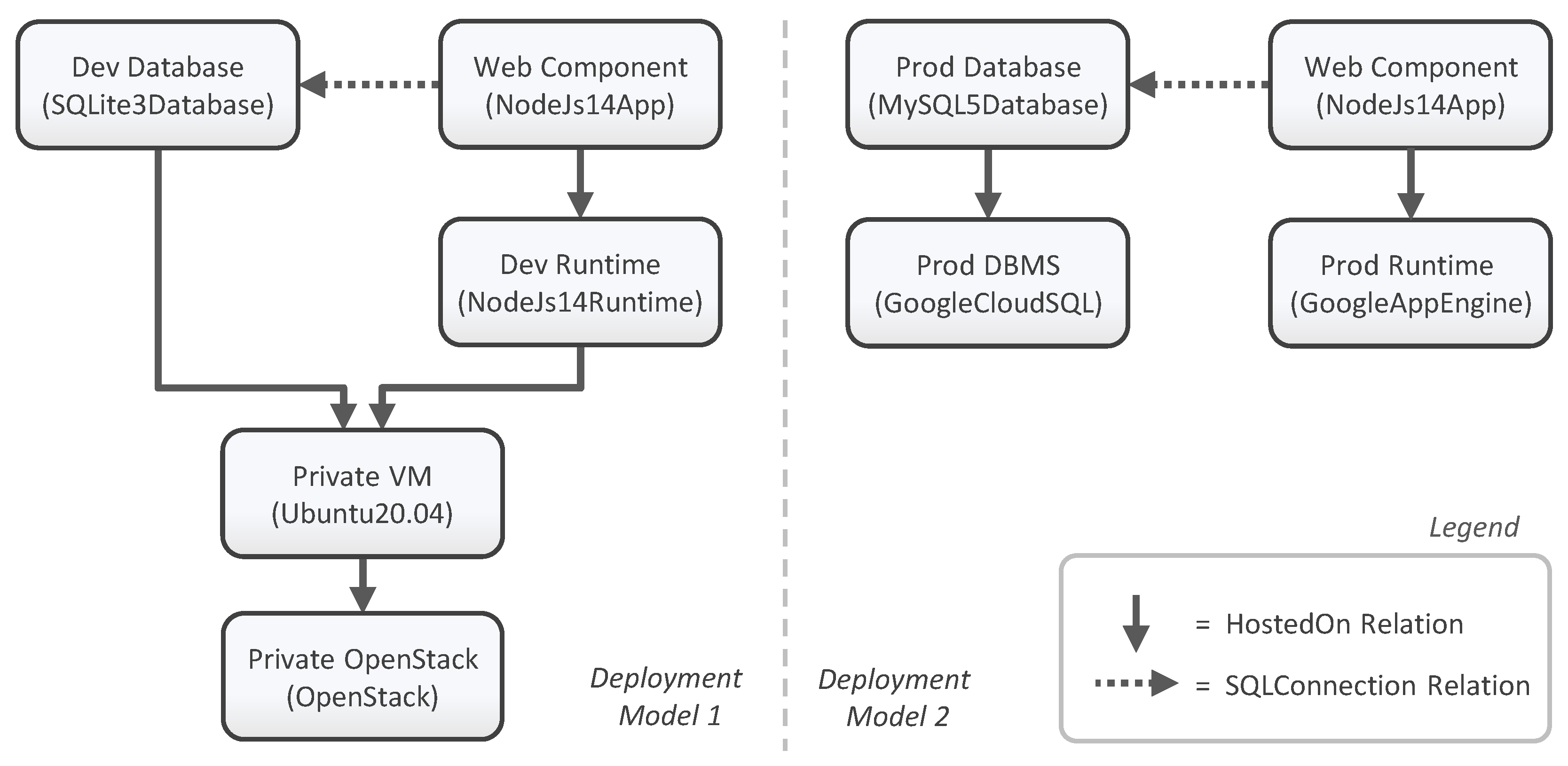
2.2. Motivating Scenario

The following motivating scenario is used throughout the paper to explain our variability modeling concepts and to show technical feasibility. We choose here a very simple scenario consisting only of two components that form the entire application to be deployed since already this simple scenario shows the drawbacks and difficulties if variants are managed in the form of individual deployment models. The motivating scenario is a simple composite application that consists of two components, (i) a web component and (ii) a database. This application can be deployed in different variants. Requirements, such as expected workload, costs, availability, development simplicity, and compliance, influence the decision on which variant to use.

During development, the deployment of the entire application should be cost efficient and fast. Therefore, often all components are simply deployed on a single virtual machine that runs on a hypervisor such as a private OpenStack as shown on the left in Figure 1. In our scenario, the web component is a NodeJs14 application that runs on a local NodeJs14 runtime that connects to a local SQLite3 database.

However, if the application has to serve production workloads all components should be hosted on managed elastic cloud service offerings. In our scenario, we select GCP as provider as shown on the right in Figure 1: The web component is hosted inside Google App Engine [5] and Google Cloud SQL [6] is used to provide a MySQL5 database. If GCP is not a suitable provider, of course also Amazon Web Services (AWS) or others could be used.

Thus, in general, any combination of suitable technologies, cloud providers, and cloud service types can be used to deploy this composite application. If many different deployment variants of a single application are required, it is infeasible to model each variant as a separate deployment model. Managing all these deployment models would be a complex, time-consuming, and error-prone task. For example, if a new version of the web component is released, the respective component must be updated in each deployment model.

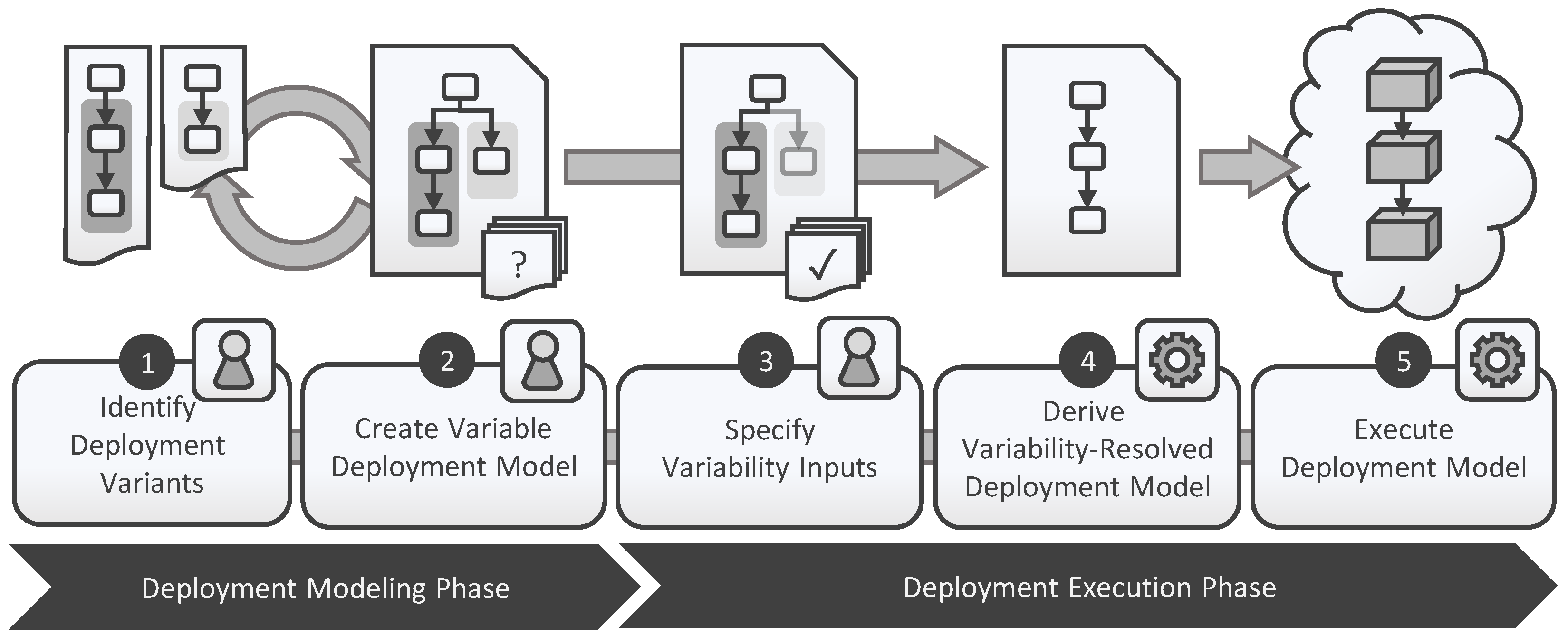
3. Variable Deployment Modeling Method

To give an overview of the idea of what Variable Deployment Models are, how they are created, and how they are used for deployment, this section presents the Variable Deployment Modeling Method, which consists of five steps. The method is split into the Deployment Modeling Phase and the Deployment Execution Phase as shown in the lower part of Figure 2. The two phases involve different user roles: while the modeling phase is typically conducted by deployment experts creating Variable Deployment Models, the execution phase can be conducted by experts as well as non-experts that want to deploy the application in a certain variant.

During the modeling phase, the first step is (i) to identify deployment variants along with their commonalities and differences. Then (ii) a Variable Deployment Model is created that describes all these variants. During the execution phase, (iii) inputs are specified that are then used in step (iv) to automatically resolve the variability and to derive an executable deployment model, i.e., the inputs are used to evaluate conditional elements in the model that are then either present or not. Finally, in the last step, (v) the derived deployment model is executed to automatically deploy the respective variant. In the next subsections, we further explain each step in more detail.

3.1. Step ➊: Identify Deployment Variants

Before a Variable Deployment Model can be created, the possible variants along with their commonalities and differences must be manually identified by a deployment expert. The result of this step is, for example, that a development variant and a production variant are required according to our motivating scenario where the development variant intends to provide a simple deployment with costs and time in mind, while the production variant requires a high-available and elastic deployment. Please note that a variant does not necessarily affect all components and relations but can differ from only a single component or configuration, for example.

3.2. Step ➋: Create Variable Deployment Model

After understanding which variants exist and which components and relations must be present in each variant, the Variable Deployment Model can be created. A Variable Deployment Model is a deployment model that has at least one conditional component or relation, which is only present if attached conditions, so-called Variability Conditions, are fulfilled. As a starting point, the Variable Deployment Model is developed for one variant and then incrementally extended with components and relations of other variants. During this process, conditions are assigned to these components and relations to ensure that they are only present in the respective variants. Variability Conditions are expressions based on Variability Inputs. In our motivating scenario, there is a single Variability Input “mode” that specifies if the application should be deployed for development or production. In contrast, in a more complex scenario, there could be various Variability Inputs, such as the legal location of the company that is responsible for this deployment or the current prices of cloud offerings. Thereby, the legal location might be used to select a compliant data storage while the prices are used to select the most cost-efficient deployment variant. Thus, Variability Inputs can be combined arbitrarily in complex conditions to model deployment variants that are highly dependent on the current context.

3.3. Step ➌: Specify Variability Inputs

This step is the first of the execution phase, in which a human operator or a system invoking the deployment selects a Variable Deployment Model and provides the required Variability Inputs. For example, a Variable Deployment Model may define the legal location of the deployment as the Variability Input, which could be important if personal data need to be stored by the application and when there are laws such as the General Data Protection Regulation that needs to be complied with. In our motivating scenario, only the Variability Input “mode” has to be specified, which is used to evaluate if the application should be deployed for development or for production.

3.4. Step ➍: Derive Variability-Resolved Deployment Model

The Variable Deployment Model as well as the Variability Inputs are then sent to the Variability Resolver. The Variability Resolver is a software component that automatically resolves the variability, i.e., it generates a Variability-Resolved Deployment Model that is a normal executable deployment model of a certain deployment technology, such as Terraform, Puppet, or TOSCA. Thus, the resulting model represents the derived deployment variant. Thereby, the Variability Resolver evaluates each condition attached to a component or relation and removes the ones whose conditions are not fulfilled. This resolver might be integrated into a deployment system that is aware of Variable Deployment Models. We provide an architecture and prototypical implementation of such a deployment system based on the TOSCA standard in Section 5.

3.5. Step ➎: Execute Deployment Model

The final step of the method is the actual deployment of the application. Therefore, a deployment system interprets the previously derived Variability-Resolved Deployment Model and executes the deployment. Since the resolved deployment model is a normal executable deployment model this deployment system must not be aware of Variable Deployment Models. If requirements change at a later stage, the execution phase can be repeated to update the running application.

4. Variable Deployment Models

This section first presents the concept of Variable Deployment Models in detail followed by a formal definition of the corresponding metamodel in Section 4.1, which provides the basis for realizing Step ➋ of our method. In Section 4.2, we introduce algorithms for resolving the variability to generate concrete executable deployment models. These algorithms are implemented by the Variability Resolver as described in Step ➍ of the method.

A Variable Deployment Model is a deployment model which has conditional elements. These are components or relations which have at least one Variability Condition assigned. Only if all Variability Conditions of a conditional element evaluate to true is the associated component or relation present in the deployment. This significantly eases handling multiple variants of a deployment since the human operator does not have to select one out of many deployment models implementing different variants, but only has to provide the required Variability Inputs.

Figure 3 shows this concept based on the motivating scenario introduced in Section 2. Instead of having two different deployment models for the two variants, the shown Variable Deployment Model contains all components and relations of both variants but associated with the Variability Conditions under which they are present in the respective deployment variant. The component “Web Component” should always be present and, thus, has no conditions assigned. However, the components “Dev Database”, “Dev Runtime”, “Private VM” and “Private OpenStack” along with their respective relations are conditional elements which should be only present in the development variant. Therefore, they have a condition assigned that evaluates if the desired deployment is intended for development. In contrast, the components “Prod Database”, “Prod DBMS”, and “Prod Runtime” along with their respective relations are conditional elements having a condition assigned that evaluates if the desired deployment is intended for production.

4.1. Variable Deployment Metamodel

This section introduces the Variable Deployment Metamodel (VDMM), which is based on EDMM introduced by Wurster et al. [1]. In the following, we first explain the underlying EDMM and introduce the required extensions for variability afterward.

EDMM defines a metamodel for declarative deployment models which was the result of an analysis of the most prominent declarative deployment technologies, including Terraform [7], Puppet [8], Kubernetes [9], and Ansible [10]. EDMM contains only modeling elements that can be mapped to all of these technologies, thus providing the greatest common denominator of all these technologies. Since our approach is based on EDMM, the approach can also be applied to these technologies. EDMM defines declarative deployment models in the form of a directed graph in which typed components are represented as colored nodes and typed relations as weighted edges. Figure 4 contains the class diagram of EDMM in the form of white boxes. Please note that this class diagram does not show the entire EDMM but only the classes required for our approach. For example, we omit the definition of Operations that are, for example, responsible for provisioning and configuring a component.

VDMM extends EDMM with classes for variability modeling which are rendered as grey boxes in Figure 4. A Variable Deployment Model represents all possible deployment variants. A deployment variant is defined as $d_i\in D_{vdm}$, where $D_{vdm}$ is the set of all executable deployment models that can be derived from a Variable Deployment Model $vdm\in \mathcal{VDM}$, where $\mathcal{VDM}$ is the set of all Variable Deployment Models.

Let $\mathcal{VDM}$ be the set of all Variable Deployment Models, then $vdm\in \mathcal{VDM}$ is defined as a tuple as follows:

$$\begin{array}{cc}\hfill vdm=& (C_{vdm},R_{vdm},C{T}_{vdm},R{T}_{vdm},typ{e}_{vdm},P_{vdm},propertie{s}_{vdm},V{I}_{vdm},\hfill \\ \hfill & CO{N}_{vdm},input{s}_{vdm},G_{vdm},condition{s}_{vdm},evaluat{e}_{vdm})\hfill \end{array}$$

(1)

We first describe the classes of EDMM as defined by Wurster et al. [1]. These classes provide the basis for declarative deployment models.

• $C_{vdm}$ is the set of Components in $vdm$. Each $c_i\in C_{vdm}$ represents a component of the application. Considering our motivating scenario, the components “Web Component”, “Dev Runtime”, and “Private VM”, for example, belong to this set.
• $R_{vdm}\mathsf{\subseteq }{C}_{vdm}\times C_{vdm}$ is the set of Relations between two components in $vdm$. Each $r_i=(c_s,c_t)\in R_{vdm}$ represents a relationship between two components of the application, whereby $c_s$ is the Source and $c_t$ the Target Component. Considering our motivating scenario, the hosting relation between the (source) component “Web Component” and (target) component “Dev Runtime”, for example, is such a relationship.
• $C{T}_{vdm}$ is the set of Component Types in $vdm$. Each $c{t}_i\in C{T}_{vdm}$ describes the semantics of a component having this type. Considering our motivating scenario, the component “Web Component”, for example, has the type “NodeJs14App” which describes, for example, that a hosting relation is required.
• $R{T}_{vdm}$ is the set of Relation Types in $vdm$. Each $r{t}_i\in R{T}_{vdm}$ describes the semantics for each relation having this type. Considering our motivating scenario, the relation between the components “Web Component” and “Dev Runtime”, for example, is of type “hostedOn” and describes that the component “Web Component” is running on the component “Dev Runtime”.
• The set of Typed Elements $E_{vdm}:=C_{vdm}\cup R_{vdm}$ is the union set of components and relations in $vdm$. Considering our motivating scenario, the components “Web Component” and “Dev Runtime”, for example, along with their hosting relation belong to this set.
• The set of Typed Element Types $E{T}_{vdm}:=C{T}_{vdm}\cup R{T}_{vdm}$ is the union of component and relation types in $vdm$. Considering our motivating scenario, the component type “NodeJs14App” and relation type “hostedOn”, for example, belong to this set.
• $typ{e}_{vdm}:E_{vdm}\to E{T}_{vdm}$ is the mapping function that assigns all components and relations in $vdm$ their respective component or relation type and, therefore, provides the semantics of typed elements. Considering our motivating scenario, the component “Web Component”, for example, is of type “NodeJs14App”.
• $P_{vdm}\mathsf{\subseteq }{\mathsf{\Sigma }}^{+}\times {\mathsf{\Sigma }}^{+}$ is the set of Properties in $vdm$. Each $p_i=(key,value)\in P_{vdm}$ describes a property of a component (type) or relation (type). Considering our motivating scenario, such properties are, for example, database credentials such as a username and password. However, properties are not shown in the figures for brevity.
• $propertie{s}_{vdm}:E_{vdm}\cup E{T}_{vdm}\to \wp \left(P_{vdm}\right)$ is the mapping function that assigns each typed element $e_i\in E_{vdm}$ and typed element type $e{t}_i\in E{T}_{vdm}$ its properties $p{s}_i\in \wp \left(P_{vdm}\right)$ in $vdm$. Considering our motivating scenario, the database connection between the “Web Component” and “Prod Database”, for example, is assigned its respective properties, such as a username and password. However, properties are not shown in the figures for brevity.

At this point, the described classes represent a deployment model according to EDMM. In the following, we introduce new classes required for variability modeling as described in our concept presented above. Thus, these new classes together with the already listed EDMM classes form the VDMM.

• $V{I}_{vdm}$ is the set of Variability Inputs in $vdm$. Each $v{i}_i\in V{I}_{vdm}$ is used inside Variability Conditions. Considering our motivating scenario, a Variability Input “mode”, for example, states if the desired deployment is for development or for production. Other Variability Inputs could ask for enabled features such as elasticity or for the legal location to select a compliant hosting offering.
• $CO{N}_{vdm}$ is the set of Variability Conditions in $vdm$. Each $co{n}_i\in CO{N}_{vdm}$ describes a Variability Condition under which a component, relation, or group is present in the deployment variant. Considering our motivating scenario, a Variability Condition “Dev”, for example, is assigned to the component “Dev Runtime” which evaluates that the Variability Input “mode” has the value “dev”. Other Variability Conditions could consider cloud offering prices.
• $input{s}_{vdm}:CO{N}_{vdm}\to \wp \left(V{I}_{vdm}\right)$ is the mapping function that assigns each Variability Condition $co{n}_i\in CO{N}_{vdm}$ the required set of Variability Inputs $vi{s}_i\in \wp \left(V{I}_{vdm}\right)$ in $vdm$ that are required to evaluate $co{n}_i$. Considering our motivating scenario, the Variability Input “mode”, for example, is assigned to the Variability Condition “Dev”.
• $G_{vdm}\mathsf{\subseteq }\wp \left(E_{vdm}\right)$ is the set of all Groups in $vdm$. Hereby, a $g_i\in G_{vdm}$ is a group that consists of components and relations in $vdm$ that are grouped to associate one or more Variability Conditions to all elements contained in this group. Considering our motivating scenario, the components “Dev Runtime”, “Dev Database”, and “Private VM”, for example, along with their relations could have been added to the same group to manage all conditional elements which are present during the development variant.
• $condition{s}_{vdm}:E_{vdm}\cup G_{vdm}\to \wp \left(CO{N}_{vdm}\right)$ is a mapping function in $vdm$ that assigns each component $c_i\in C_{vdm}\mathsf{\subseteq }{E}_{vdm}$, relation $r_j\in R_{vdm}\mathsf{\subseteq }{E}_{vdm}$, and group $g_k\in G_{vdm}$ the Variability Conditions $con{s}_l\in \wp \left(CO{N}_{vdm}\right)$ under which it is present in the deployment variant. If a component, relation, or group have no Variability Conditions, the mapping function assigns them the empty set. Considering our motivating scenario, the Variability Condition “Dev”, for example, belongs to this set.
• $evaluat{e}_{vdm}:CO{N}_{vdm}\times \wp \left(V{I}_{vdm}\right)\to \{true,false\}$ is the function in $vdm$ that assigns under the Variability Inputs $v{i}_i\in \wp \left(V{I}_{vdm}\right)$ a Variability Condition $co{n}_i\in CO{N}_{vdm}$ either $true$ or $false$. Considering our motivating scenario, this function evaluates, for example, regarding the Variability Condition “Dev” if the Variability Input “mode” has the value “dev”.

4.2. Algorithms for Resolving Variability

This section presents algorithms to transform a Variable Deployment Model into a Variability-Resolved Deployment Model as required in Step ➍ of our method. These include the algorithms resolveVariability for deriving a deployment model from a Variable Deployment Model, checkElementPresence for checking the presence of an element, and checkConsistency for checking the consistency.

4.2.1. Variability Resolving Algorithm

The algorithm resolveVariability in Algorithm 1 resolves the variability and derives a Variability-Resolved Deployment Model from a Variable Deployment Model. First, in Line 2 all components are collected which are present in the derived deployment model, Line 3 collects all present relations. Thereby, the conditions that are assigned to components and relations are evaluated using the checkElementPresence algorithm introduced in Section 4.2.2. In Line 6, the derived deployment model is constructed from the set of present components and relations. The remaining elements, such as the set of component types, can be directly taken from the Variable Deployment Model. The derived deployment model does not have any variability and conforms to EDMM. Therefore, since EDMM models can be automatically transformed to concrete deployment technologies such as Terraform [11] the derived deployment model can be executed by standard deployment technologies that are not aware of our variability concepts.

Algorithm 1 resolveVariability ($vdm\in \mathcal{VDM}$): $d\in D_{vdm}$

1: // Calculate all present components and relations

2: $C_d:=\left\{c_i\right|c_i\in {\mathit{C}}_{\mathit{vdm}}:\mathit{checkElementPresence}\left(c_i\right)=\mathit{true}\}$

3: $R_d:=\left\{r_i\right|r_i\in {\mathit{R}}_{\mathit{vdm}}:\mathit{checkElementPresence}\left(c_i\right)=\mathit{true}\}$

4:

5: // Return Deployment Model

6: return  $\{C_d,R_d,{\mathit{CT}}_{\mathit{vdm}},{\mathit{RT}}_{\mathit{vdm}},{\mathit{type}}_{\mathit{vdm}},{\mathit{P}}_{\mathit{vdm}},{\mathit{properties}}_{\mathit{vdm}}\}$

4.2.2. Element Presence Check Algorithm

The algorithm checkElementPresence in Algorithm 2 checks if an element is present in a deployment by evaluating assigned conditions. Therefore, all conditions which are assigned to the element are collected. Conditions are either directly assigned to the element (see Line 2) or indirectly by a group (see Lines 5–7). The element is present if all assigned conditions are fulfilled (see Line 10).

Algorithm 2 checkElementPresence($e\in E_{vdm}$, $vdm\in \mathcal{VDM}$): $b\in \{true,false\}$

1: // Capture all conditions which are assigned to e

2: $cons:=condition{s}_{vdm}\left(e\right)$

3:

4: // Add all conditions which are assigned to the groups of e

5: for all ($g_i\in \left\{g_i\right|g_i\in {\mathit{G}}_{\mathit{vdm}}:e\in g_i\})$ do

6:     $cons:=cons\cup {\mathit{conditions}}_{\mathit{vdm}}\left(g_i\right)$

7: end for

8:

9: // Check that all conditions evaluate to true

10: return  $\left(\forall co{n}_i\in cons:{\mathit{evaluate}}_{\mathit{vdm}}({\mathit{con}}_{\mathit{i}},{\mathit{inputs}}_{\mathit{vdm}}\left(co{n}_i\right))=\mathit{true}\right)$

4.2.3. Consistency Check Algorithm

Inconsistencies might occur in the derived Variability-Resolved Deployment Model. If, for example, a component has multiple conditional hosting relations to several components but their conditions do not exclude each other, i.e., more than one of these hosting relations have all their assigned conditions fulfilled, the component must be hosted on multiple components at the same time which is not possible. Of course, such overlapping conditions are a clear modeling mistake and must be avoided during modeling. However, if the variability is high, such modeling errors might occur. Therefore, we introduce the algorithm checkConsistency in Algorithm 3 that executes four checks regarding the consistency of the derived model. The first two checks verify that the source component and target component of each relation in the derived model is also present in the derived model (see Lines 2–4 and 7–9). It is possible that, for example, a relation is present while the target component is not if all conditions of the relation evaluate to true but the ones assigned to the target component do not. The third check verifies that each component in the derived model has at maximum one hosting relation in the derived model (see Lines 12–14). Multiple hosting relations can occur, for example, when their assigned conditions do not exclude each other. Thereby, the check allows components without hosting relations, such as a basic infrastructure virtualization layer as OpenStack, since these are typically not managed by the deployment model. The last and fourth check verifies that each component in the derived model has a hosting relation if the component has at least one hosting relation in the Variable Deployment Model (see Lines 17–19). Thereby, we assume that if a component has a hosting relation in any variant then a hosting relation is always required. Considering our motivating scenario, the component “Web Component”, for example, always requires a hosting relation while having two conditional hosting relations in the Variable Deployment Model. If none of these relations are present in the derived model, then the deployment model cannot be executed.

Algorithm 3 checkConsistency($d\in D_{vdm}$, $vdm\in \mathcal{VDM}$): $b\in \{\mathit{true},\mathit{false}\}$

1: // Ensure that each relation source exists

2: if  $\left(\exists r_i=(s,t)\in R_d:s\notin C_d\right)$then

3:     return $\mathit{false}$

4: end if

5:

6: // Ensure that each relation target exists

7: if  $\left(\exists r_i=(s,t)\in R_d:t\notin C_d\right)$then

8:     return $\mathit{false}$

9: end if

10:

11: // Ensure that every component has at maximum one hosting relation

12: if  $$\begin{gathered} \left(\exists c_i\in C_d\exists r_j=(c_i,a)\in R_d\exists r_k=(c_i,b)\in R_d: \\ {r}_j\ne r_k\wedge {\mathit{type}}_{\mathit{d}}\left(r_j\right)={\mathit{type}}_{\mathit{d}}\left(r_k\right)=\mathit{hostedOn}\right)\mathbf{then} \end{gathered}$$

13:     return $\mathit{false}$

14: end if

15:

16: // Ensure that every component that had a hosting relation previously still has one

17: if  $$\begin{gathered} \left(\exists c_i\in C_d\exists r_j=(c_i,a)\in R_{vdm}\exists !r_k=(c_i,b)\in R_d: \\ {\mathit{type}}_{\mathit{vdm}}\left(r_j\right)={\mathit{type}}_{\mathit{d}}\left(r_k\right)=\mathit{hostedOn}\right)\mathbf{then} \end{gathered}$$

18:     return $\mathit{false}$

19: end if

20:

21: // All checks passed

22: return  $true$

5. Prototypical Validation and Case Study

To validate the technical feasibility of the method presented in Section 3 and the concept of Variable Deployment Models, we implemented a prototype based on the Topology and Orchestration Specification for Cloud Applications (TOSCA) [4]. TOSCA is an official OASIS standard for automating the deployment and management of cloud applications in a technology-independent and vendor-neutral manner. For this purpose, we (i) first introduce Variability4TOSCA, which is an extension of the TOSCA Simple Profile in YAML Version 1.3 [4] that supports VDMM introduced in Section 3. Afterward, we (ii) present the architecture, prototypical implementation, and benchmark of OpenTOSCA Vintner  [12], which is a Variability4TOSCA Deployment System that enables automating Steps ➍ and ➎ of our method. Thus, OpenTOSCA Vintner enables automatically transforming Variability4TOSCA models into standard-compliant TOSCA models that can be executed by standard-compliant TOSCA orchestrators. We demonstrate this by employing the open-source orchestrators xOpera [13] and Unfurl [14] for executing the generated TOSCA models. Finally, we (iii) conduct a case study and apply our method to our motivating scenario.

5.1. Variability4TOSCA: An Extension of the TOSCA Standard

To support our variability concept in TOSCA Simple Profile in YAML Version 1.3 [4] we present our TOSCA extension Variability4TOSCA. The full specification can be found on our GitHub repository together with the source code of OpenTOSCA Vintner [12].

5.1.1. Mapping EDMM to TOSCA

Since the EDMM classes are part of VDMM, we first describe how they can be mapped to TOSCA. According to Wurster et al. [1,15], EDMM can be mapped to TOSCA as follows: In TOSCA, the deployment of an application is described as a Topology Template. Such a Topology Template is the equivalent of our deployment model and consists of Node Templates and Relationship Templates. These templates describe the application components along with their relations. Thereby, components of our deployment model correspond to Node Templates and relations to Relationship Templates. Node Types and Relationship Types semantically describe Node Templates and Relationship Templates. Therefore, component types and relation types correspond to Node and Relationship Types. Node Templates and Types can be configured using Properties that are equivalent to properties of components and their types. The same applies to Relationship Templates and Types. A more detailed description of TOSCA is given by Binz et al. [16,17].

5.1.2. Extending TOSCA for VDMM

To support VDMM, we extend the TOSCA standard as follows. Variability4TOSCA is based on TOSCA Simple Profile in YAML Version 1.3 [4] and introduces conditional elements. Thereby, we extend the Topology Template with a Variability Definition that contains Variability Inputs.

A Variability Condition is modeled as a Boolean expression producing a Boolean value, i.e., true or false, when evaluated. Thereby, Boolean, arithmetic, and constraint operators along with intrinsic functions can be used inside conditions. These include, among others, and, or, not, xor, implies, getVariabilityInput, getVariabilityCondition, getElementPresence, add, sub, concat, equal, and greaterThan operators.

To model conditional elements, we extend Node Templates, Requirement Assignments, and Group Definitions with the capability to contain a Variability Condition. Requirement Assignments are entities in TOSCA that assign the Source and Target Node Template to a Relationship Template, while Group Definitions are used to group Node Templates. Furthermore, we extend Group Definitions by allowing Requirement Assignments to be group members. An example of a conditional element from our motivating scenario is shown in Listing 1 in Line 13: The Node Template “DevRuntime” is only present if the Variability Condition in Line 15 is true, thus, if the Variability Input “mode” equals “dev”. It is also possible to assign multiple conditions by specifying a list. In such a case, the conditions are combined using the logical and operator. To reduce repetitiveness, a Variability Condition, or even only parts of the condition, can be defined globally as part of the Variability Definition and then referenced on multiple occasions.

Listing 1. Excerpt of the Topology Template of our motivating scenario showing modeled Variability Conditions for the runtime of the web component as well as hosting relations to them.

1 topology_template: 2   node_templates: 3     WebComponent: 4       type: NodeJs14App 5       requirements: 6         - host: 7             node: DevRuntime 8             conditions: {equal: [{get_variability_input: mode}, dev]} 9         - host: 10             node: ProdRuntime 11             conditions: {equal: [{get_variability_input: mode}, prod]} 12       ... 13     DevRuntime: 14       type: NodeJs14Runtime 15       conditions: {equal: [{get_variability_input: mode}, dev]} 16       ... 17     ProdRuntime: 18       type: GoogleAppEngine 19       conditions: {equal: [{get_variability_input: mode}, prod]}) 20       ... 21     ... 22   ... 23 ...

5.2. System Architecture for a Variability4TOSCA Deployment System

In this section, we present a conceptual system architecture for a Variability4TOSCA Deployment System, which is implemented by our OpenTOSCA Vintner prototype described in the next section. Our system architecture is shown in Figure 5 and consists of the following components. The Variability4TOSCA Model Importer parses a Variability4TOSCA model and transforms it into an internal data structure. To derive a Variability-Resolved Deployment Model, the Variability Resolver implements the algorithms from Section 4.2. A derived model is then exported as TOSCA conform deployment model using the TOSCA Model Exporter.

The Deployment Manager executes the deployment model using Orchestrator Plugins which communicate with TOSCA conform orchestrators. Therefore, our architecture is not restricted to a specific TOSCA orchestrator. TOSCA models and definitions, such as TOSCA Type Definitions and Topology Templates, are stored in the TOSCA Models database. Information about instances of a TOSCA model, such as used Topology Templates, are stored in the Instance Models database.

5.3. OpenTOSCA Vintner

OpenTOSCA Vintner implements the system architecture introduced above. The system is written in NodeJs and can be invoked using the command line or a REST API. The Variability Resolver can be also used as a standalone tool and, thus, be integrated into any toolchain. The Deployment Manager is able to deploy applications using xOpera and Unfurl. Thereby, we implemented a plugin for Linux and for Windows using the Windows-Subsystem for Linux (WSL) [18]. To store TOSCA models and instance models, the filesystem is used. The prototype does not support the inheritance of the TOSCA type system as it is not required for our approach and expects that hosting relations are named “host” as commonly done in the TOSCA specification. The source code and documentation can be found in our repository.

5.4. Case Study Based on the Prototype

This section presents a detailed case study in which we apply the Variable Deployment Modeling Method presented in Section 3 to the motivating scenario introduced in Section 2. A step-by-step guide, including corresponding TOSCA definitions, is provided in our repository.

In Step ➊ of our method, we first identify that we require a development variant and a production variant. With costs and simple installation in mind, the development variant deploys all components on a single virtual machine on a private OpenStack instance. For the database, we use a lightweight SQLite3 database because it is easier to manage compared to MySQL. Since an unexpected workload is expected during production, the web component and the database are deployed on GCP in the production variant.

To create the Variability4TOSCA model in Step ➋, we start with creating the development variant, i.e., we model all components and relations as shown in Figure 1 on the left. To integrate the production variant, the components “Prod Database”, “Prod DBMS” and “Prod Runtime” are added along with their relations. At this stage, the web component has two hosting relations and two database connections. Therefore, we define the Variability Input “mode” and assign a condition that checks if “mode” equals “dev” to the components and relations that are only present in the development variant (see Listing 1). Analogously, we assign a condition checking if “mode” equals “prod” to the components and relations that are only present in the production variant. Since the component “Web Component” should always be present, it does not have any conditions assigned. The final Variability4TOSCA model is shown in Figure 3. Hereby, the manual modeling phase of the method is completed.

In the execution phase, we want to deploy the application in the development variant. Therefore, we import the created Variability4TOSCA model to OpenTOSCA Vintner and assign the Variability Input “mode” the value “dev” in Step ➌. The Variability Resolver receives the model and our input in Step ➍. Since only the conditions that check if “mode” equals “dev” evaluates to true, the resolver removes all components and relations whose conditions check for “prod”. The resulting standard-compliant TOSCA model corresponds to the development variant given in Figure 1 on the left. In the final Step ➎, we select xOpera or Unfurl as the TOSCA orchestrator to execute the deployment in a fully automated manner.

This case study can be used to evaluate different aspects of our presented approach. First, the motivating scenario introduced in Section 2 can be realized using Variability4TOSCA, which shows that our extension of the TOSCA standard provides all required features for this kind of scenario. Moreover, the case study also demonstrates that our prototypical implementation OpenTOSCA Vintner is able to automatically transform Variability4TOSCA models for a given set of provided Variability Inputs into a standard-compliant TOSCA model that can be executed by unmodified TOSCA orchestrators, in this case, xOpera or Unfurl. Thus, these results pave the way for executing different deployment variants in practice on top of existing toolchains.

5.5. Benchmark Evaluation of the Variability Resolver Prototype

To further evaluate our concept and prototype, we ran benchmark tests whose results are given in

Table 1. Benchmark results of the Variability Resolver prototype (Since tests 1–7 are in-memory, respective file measurements are not available).

Test	Seed	Templates	Median	Median/Template	File Size	File Lines
1	10	40	0.295 ms	0.007 ms	n/a	n/a
2	250	1000	4.045 ms	0.004 ms	n/a	n/a
3	500	2000	4.329 ms	0.002 ms	n/a	n/a
4	1000	4000	7.383 ms	0.002 ms	n/a	n/a
5	2500	10,000	29.436 ms	0.003 ms	n/a	n/a
6	5000	20,000	63.307 ms	0.003 ms	n/a	n/a
7	10,000	40,000	137.353 ms	0.003 ms	n/a	n/a
8	10	40	3.335 ms	0.083 ms	14 kB	360
9	250	1000	39.033 ms	0.039 ms	351 kB	8760
10	500	2000	88.504 ms	0.044 ms	704 kB	17,510
11	1000	4000	225.444 ms	0.056 ms	1.409 MB	35,010
12	2500	10,000	947.011 ms	0.095 ms	3.553 MB	87,510
13	5000	20,000	3.185 s	0.159 ms	7.125 MB	175,010
14	10,000	40,000	11.345 s	0.284 ms	14.270 MB	350,010

. The to-be-tested Topology Templates are generated based on a seed. For example, a seed of 1000 generates the 1000 Node Templates $a_0,a_1,\dots ,a_{999}$, which have a condition assigned that evaluates to true. In addition, 1000 Relationship Templates $r{a}_0=(a_0,a_1),r{a}_1=(a_1,a_2),\dots ,r{a}_{999}=(a_{999},a_0)$ are generated, which connect one Node Template $a_i$ and the next Node Template $a_{i+1mod1000}$ and which have a condition assigned, which evaluates to true. Furthermore, the 1000 Node Templates $b_0,b_1,\dots ,b_{999}$ are generated, which have a condition assigned that evaluates to false. Additional 1000 Relationship Templates $r{b}_0=(a_0,b_0),r{b}_1=(a_1,b_1),\dots ,r{b}_{999}=(a_{999},b_{999})$ are generated which connect the Node Template $a_i$ with the Node Template $b_i$ and which have a condition assigned which evaluates to false. In total, 4000 templates are generated consisting of 2000 Node Templates and 2000 Relationship Templates. After resolving the variability, only the 1000 Node Templates $a_0,a_1,\dots ,a_{999}$ along with the 1000 Relationship Templates $r{a}_0,r{a}_1,\dots ,r{a}_{999}$ between them are present.

The time for transforming the Variability4TOSCA model into an internal data structure, resolving the variability, running the consistency check, and transforming the Topology Template into a TOSCA Simple Profile in YAML Version 1.3 model is measured. Thereby, the Variability4TOSCA model is already loaded as JSON in memory. To remove outliers, the median of 10 test runs is used. The benchmark results of all in-memory tests are given in Table 1 (see tests 1–7). A Topology Template consisting of 40 templates (20 Node Templates and 20 Relationship Templates) is processed within 0.295 ms, a Topology Template consisting of 40,000 templates (20,000 Node Templates and 20,000 Relationship Templates) within 137.353 ms. As seen by the median per template column in Table 1 and Figure 6 on the left, the time used for processing scales slightly non-linear.

In another test set, we additionally measured the time which is needed to read and write the Topology Template files which also includes YAML parsing. These tests take significantly longer mainly due to the parsing of YAML. The benchmark results of these tests are given in Table 1 (see tests 8–14). A Topology Template consisting of 40 templates is processed within 3.335 ms, a Topology Template consisting of 40,000 templates within 11.345 s. The file of the Topology Template consisting of 400,000 templates has a size of 14.270 MB and consists of 350,010 lines. As a result, the processing scales worse (see Table 1 and Figure 6 on the right). Such Topology Templates are already huge, possibly representing a single deployment consisting of thousands of servers and their hosted components along with databases. The required time for processing is negligible in comparison to the time required to actually provision such huge topologies. Based on our experience, creating, for example, a MySQL5 DBMS on GCP takes several minutes.

The tests have been executed on commodity hardware; to be specific, on Windows 10, an i7-6700K CPU 4x 4.00GHz, 2133MHz DDR4 RAM, and NVMe M.2 SSD. Due to the single-threaded nature of NodeJs, only a single core is used. The performance could be further improved by using better hardware, threading, or a more efficient language, such as Go. Refactoring the algorithm could also improve the performance. However, at the current stage, we prefer understandability over performance.

6. Related Work

In the following, we discuss related work considering different research topics, such as product line engineering, context-aware deployment, optimization, and self-adaptation.

6.1. Software Product Line Engineering

Software Product Line Engineering (SPLE) [19,20,21,22] is an approach to manage and derive different variants of software, the product. There are two phases: domain engineering and application engineering. During domain engineering, a requirements analysis is conducted to create the product line along with a variability model, such as feature models [23] or orthogonal variability models (OVM) [19], which represent the problem space. A feature model describes in a single tree which common and variable features are available and which dependencies between them exist [23]. In comparison, an OVM consists of multiple variant points which represent variable features and, therefore, do not consider common features [19]. During application engineering, another requirements analysis is conducted to select the features and generate the desired product using artifacts from the product line, which represent the solution space. Compared to our work, we have a similar high-level process. The Variable Deployment Model and the corresponding algorithms can be seen as the solution space in SPLE terminology. Furthermore, we make use of conditional elements, which is an established technique for the solution space. In contrast, we focus on deploying composite multi-cloud applications and not on the generation of software. However, these concepts can be combined. For example, before a component is deployed, corresponding software can be generated based on information contained in the deployment model. Thus, our approach sits between the variability modeling and the generation of corresponding software and, therefore, bridges the gap between SPLE and deployment.

Groher and Voelter [24] presented a general method to integrate feature-based variability and structural models in the context of product line engineering. They differentiated between positive and negative variability. Based on a feature selection, positive variability extends a base model by optional elements, whereas negative variability removes optional elements from a base model. Our approach can be classified as negative variability. Similar, Czarnecki et al. [25] discussed the combination of SPLE and Model Driven Software Development (MDSD). However, deployment was not discussed.

Czarnecki and Antkiewicz [26] presented a general approach for integrating feature models for negative variability. They discussed how feature models and a model template can be used to generate a desired model. Thereby, elements of the model template were assigned with presence conditions, e.g., Boolean expressions over the feature selection. If an element is not present, its contained elements are also not present. They also propose different kind of default presence conditions. For example, if an element is removed, outgoing relations should also be removed, even if they have no presence conditions assigned. Furthermore, meta-expressions can be used to calculate, for example, properties, such as names. After evaluating the presence conditions, they further process the model to patch or simplify the model. They show their concept based on UML 2.0 class and activity diagrams. We also make use of the concept of presence conditions but explicitly in the context of deployment models, which was not focused on by Czarnecki and Antkiewicz [26]. In contrast to their work, we provide a formal metamodel and corresponding algorithms.

Extending UML with variability using stereotypes has been researched in several related work [27,28,29,30,31,32]. In general, they introduced optional, variant point, alternative, required or exclusive stereotypes with or without the possibility to model constraints between components. In comparison, we assign conditions directly to components and relations of a deployment model.

Ferko et al. [33] reported their experience from generating configuration files from the railway domain. They used feature models in combination with a translator file, which eventually produces XML configurations that describe the product, a train. The translation file consists of a set of parameters and corresponding values along with conditions on selected features. However, they do not generate deployment configurations.

In programming languages, such as C and Java, there also exist preprocessors that enable conditional compilation, e.g., to include specific parts of the code only if a specific condition holds true [34,35,36]. Conditional compilation along with feature models was, for example, used by Cavalcante et al. [37] to generate application code that is specific for the used cloud offerings. They focused on the generation of code, while our approach focuses on the deployment of already built components and their relations. However, these concepts can be integrated into our approach by generating software based on the information contained in the deployment model before the respective components are deployed.

Using variability models from SPLE to model deployment variants is a widely used approach [22,38,39,40,41,42,43,44,45]. Thereby, multiple variability models along with dependencies between them can be used to manage different aspects of variability. However, the focus of these related work is on modeling variability in the problem space, e.g., functional and non-functional capabilities and requirements of applications in the form of multiple combined feature models. In contrast, we focus on the modeling of the application topology in the solution space and especially address the deployment of applications in detail. Since modeling the problem space complements the solution space these related work may complement our approach. For example, the feature selection of a feature model can be used as Variability Inputs for our Variability Resolver.

6.2. Variable Composite Applications

Mietzner has conducted several research studies in the field of deployment of composite applications considering topics such as variability and multi-tenancy. In the following, we present his research and discuss it in the context of our work.

Mietzner [46] addressed the problem of managing variability of applications with a focus on multi-tenancy. Several concepts of SPLE were used. An application is modeled using an application model which consists of components and their hosting relations. Multi-tenancy patterns can be assigned to components [46,47,48]. For example, a component can be shared across different deployments of different tenants. Variability is modeled using a variability model which is based on OVM and consists of variability points [19,45,46]. These variability points have different alternatives, which can be chosen from. Examples are the RAM size of a virtual machine or the branding name that should be displayed on a website. Enabling conditions state which alternatives are allowed. Thereby, complex dependencies between variability points are possible. For example, if alternative A is chosen for the variability point B, only the alternative C of variability point D is allowed. The application and variability model was also used in later work to dynamically bind services during runtime in the context of service composition [49], while Koetter et al. [50,51] made use of the variability model in the context of compliance.

In addition, Mietzner et al. generated customization flows which guide through the selection of alternatives and ensure the completeness and correctness of the selection [46,52]. There are different selection phases. For example, one phase is used by the provider of the deployment system to restrict the available infrastructure, while another phase is used by the tenant for tenant-specific configurations, such as branding or passwords. The chosen alternatives are then used to modify the implementation files of components.

Furthermore, Mietzner et al. considered multi-tenancy patterns in which components are either bound to already running components or need to be deployed [46,47,53]. For example, instead of deploying a new component, a new tenant along with tenant-specific configurations is registered at an already running component. This binding is automatically done and respected during deployment. Different optimization algorithms can be used, e.g., to reduce costs or to distribute the expected workload [46,54]. However, they do not provide such algorithms. A provisioning flow provisions components using component flows while respecting hosting relations and relations introduced by variability point dependencies [46,55]. Component flows expose a unified provisioning and management interface, which is used for lifecycle management of the components. In a later work, the overall concept was further extended with triggers, e.g., to scale components up or down [56].

In comparison to our work, we model variability inside a deployment model. Thereby, we do not focus on multi-tenancy but on modeling conditional components and their relations. This is not explicitly possible in the concept proposed by Mietzner et al., where variability targets the implementation files of components and not the application model. Furthermore, our deployment model is not only restricted to hosting relations but allows to model other relations, such as SQL connections.

The concept by Mietzner et al. for customization flows for ensuring completeness and correctness could be integrated into our concept. Having such a concept would enable us to omit our consistency check. However, such a check is still a valuable sanity check since modeling variability point dependencies is complex and error prone. We also do not further specify different phases for binding variability. However, the different phases proposed by Mietzner et al. might be used inside our phase in which Variability Inputs are specified. Furthermore, Mietzner et al. defined his own custom metamodel, whereas our deployment model is based on EDMM [1] and, therefore, can be mapped to TOSCA, Terraform, Ansible, Kubernetes, Docker Compose and more deployment technologies [1,11].

6.3. Context-Aware Deployments

In the following, we discuss related work, which focuses on context-aware deployments, such as self-adaptive systems.

Saller et al. [42] presented an approach for the context-aware adaptation of dynamic software product lines. They combined a classical feature model with a feature model representing the context. Dependencies between these two models state whether a feature can be used under a certain context. These models are used to adapt applications at runtime by monitoring the context and adapting the currently active features. In comparison to our work, they operated on feature models to directly derive the adaptation steps, while we generate a declarative deployment model which contains the application structure along with all components, relations, and configurations.

Le Nhan et al. [57] used a feature model for provisioning virtual machines which specifies available operating systems and software. The feature selection was then transformed into Chef configurations which install the expected software on the virtual machine. However, they were only restricted to a single virtual machine at a time, whereas we generate a deployment model which may consist of several components, such as virtual machines, databases or even other cloud offerings, such as Function-as-a-Service.

Quinton et al. [58] presented the concept of using a Cloud Knowledge Model to automatically select features of a feature model representing a cloud provider which finally results in the deployment of an application. Thereby, the Cloud Knowledge Model is an abstract view on available cloud offerings and is mapped to the cloud provider feature models. The selected features have assets such as configuration files or deployment scripts, which are then executed. In comparison, we generate a declarative deployment model based on conditional elements which is then executed.

Gui et al. [59] proposed a framework for adaptive real-time applications for OSGi. Their deployment model consists of components and communication relations and allows to enable or disable components based on a Boolean flag. In comparison, we explicitly model the conditions under which components and relations are present. Furthermore, our model is not focused on OSGi, allows to model any relations between components, and includes the management of hosting components.

Anthony et al. [60] presented a middleware for a self-configuring automotive control system. Software components are configured by policies that are loaded into the components. These policies execute actions based on information monitored by the middleware. In comparison, they assigned conditions to actions that should be triggered to adapt the application, whereas we assign conditions to components and relations to derive a model of the desired application.

Alkhabbas et al. [61] presented a goal-driven approach for self-adaptive systems for Internet of Things (IoT). Their framework is based on MAPE-K [62], which includes monitoring, analyzing, planning, and executing components along with a knowledge base. For example, a user defines the goal to adjust the light level in a meeting room. A deployment planner generates a topology by mapping required software components to existing hardware components while considering expected and current workload. In contrast, they expected that hardware components already exist, whereas we are able to provision, e.g., virtual machines. Furthermore, they only simulated the deployment inside their prototype, whereas we actually deployed our motivating scenario.

Ayed et al. [63] presented an approach for context-aware deployments of component-based applications on top of existing deployment technologies by using a deployment model that is platform independent. The deployment model consists of components and communication relations. Components are semantically described by types that define their interface, properties, implementations, component dependencies, and placement constraints regarding hardware. Software components are automatically matched to existing hardware components during deployment. Thereby, properties, implementations, dependencies, and placement constraints may have conditions on the context. Furthermore, the components and relations can have conditions assigned which specify if the component or relation is present in the deployment. They also detect inconsistencies such as multiple assignments of the same property or missing connection targets already during design time [64], whereas we check for inconsistencies during the deployment phase. However, they focus on software components and dynamic placement of software components to hardware components and expect that hardware components already exist. In contrast, our deployment model also allows to model, e.g., hardware components that should be automatically provisioned. Furthermore, our deployment model is based on EDMM [1] and, therefore, can be mapped to TOSCA, Terraform, Ansible, Kubernetes, Docker Compose, and more deployment technologies [1,11].

Atoui et al. [65] integrated feature models into a deployment model specialized for Network Function Virtualization (NFV) infrastructures. They represented the deployment model as a tree whose nodes are, for example, virtual compute nodes or virtual storage, and relations, such as composition, allocation, and connection. In addition, the deployment model includes OR and XOR gateways. These gateways state which subtrees can be selected. In comparison, our deployment model does not require a tree-like structure, is not specialized for NFV, and does not include such gateways but complex conditions assigned to components and relations.

Sáez et al. [66] presented a utility function to select a hosting stack for each business component based on key performance indicators. However, only the underlying hosting stack is variable, whereas in our concept, also business components are variable. Furthermore, we provide a formal metamodel along with algorithms to derive a deployment model.

Johnsen et al. [67] combined the functional and deployment variability concepts of Abstract Behavioural Specification (ABS) [68]. ABS is a specification for modeling the behavior of concurrent and distributed processes of software systems in a Java-like syntax. Following SPLE and delta-oriented programming [69,70], functional variability is modeled using a feature model for a delta-oriented base model. Selected features are linked to deltas which are applied to the base model to derive the desired product. Deployment variability refers to execution costs of process statements and resource capacities of compute nodes. The concepts are combined by integrating the feature model for functional variability with a feature model for execution costs and another one for resource capacities. As a consequence, deltas patch the base model not only regarding functionality but also regarding execution costs and resource capacities. In a given example, a MapReduce [71] master uses this information to decide which and how many workers to use. This delta-oriented approach is fundamentally different from our approach to generate the desired outcome since they add new elements to a common base model while we remove elements from a model containing all possible elements. Furthermore, we focus on modeling conditional components and relations inside a deployment model which is not only restricted to compute nodes.

Hochgeschwender et al. [43] presented a feature-oriented Domain-Specific Language (DSL) to be used in a model-driven engineering-based development process for configuring robot software architecture in the context of the BRICS robot application development process (RAP) [72]. The DSL enables to declaratively describe the deployment in a vendor-neutral manner. Thereby, a feature model describes features whose selection is used along with a resolution model to transform a template system model into the desired architecture. In comparison to our work, they focused on robotics, while we do not restrict to any domain. Furthermore, our approach is not restricted to a specific DSL.

Breitenbücher et al. [73] presented a method to transform a deployment model depending on the context by applying graph transformations. Thereby, context refers to the state and structure of the application. Management plans are then automatically generated and executed to provision and manage the application. In comparison, we do not apply graph transformations but use conditional elements and refer, for example, to costs or scalability as context.

Terraform and Ansible support conditional components and relations. In the following, we briefly discuss their concepts since we mentioned them previously. In Terraform, the count attribute [74] can be used in resource or module blocks to model conditional components. A corresponding numeric expression sets the value of count either to zero or one. This expression might be based on user-provided inputs. Relations between components are modeled using the depends_on attribute of a component or implicitly by accessing attributes of other resources. However, conditions cannot be assigned to relations. They are present as long as their source component is. This restriction does not apply to our concept. Furthermore, we support, for example, the intrinsic function getElementPresence that can be used inside an expression to specify a condition with respect to the presence of any other conditional element.

In Ansible, conditional components can be modeled using the when attribute [75] which conditionally includes components represented by playbooks [1]. The corresponding expressions use Jinja2 [76] and might be based on host facts or user-provided inputs. Relations between components are modeled implicitly by imports [1]. The same considerations which apply to Terraform also apply to Ansible. In future work, we plan to analyze the variability concepts of other popular deployment technologies and use our approach as an enabler for technologies that are not aware of such variability concepts.

6.4. Incomplete Deployment Models

Our approach explicitly models the complete deployment model, i.e., each possible component and relation along with their configurations. In contrast, the following approaches do not explicitly model the complete deployment model but use, for example, abstract components, patterns, and/or automatic completion. These approaches complement each other and can be integrated into our approach especially since some of them are based on TOSCA [77,78,79,80,81,82]. For example, business-related components can be assigned with conditions, while the underlying hosting stack is automatically completed or refined using patterns. We plan to integrate some of these concepts into our approach in future work.

Harzenetter et al. [77,78] presented an approach to model and execute deployment models using technology-agnostic and vendor-neutral cloud patterns, such as elastic platforms. Thereby, patterns are abstract components inside the deployment model, which are further refined into concrete components. For example, a user application is hosted on an elastic platform pattern which is refined to the components “AWS Elastic Beanstalk Environment” and “AWS Elastic Beanstalk”.

Kuroda et al. [83] presented a method to transform an abstract topology into a concrete deployable topology. The abstract topology is transformed based on actions that replace a subgraph with another subgraph until the topology consists only of concrete components and relations. A search-based algorithm is used to decide which actions should be executed. They proved the feasibility of their method by implementing a prototype that is based on TOSCA.

Knape [79] presented a method to automatically select and deploy software components in the cloud by combining feature models and TOSCA. Thereby, the TOSCA model only consists of software components having an abstract type. Each component expresses constraints that are used to select a cloud offering along with its configuration based on a component-specific feature model. Based on this selection, the component type is changed to a concrete type which results, for example, in the deployment of the component on GCP.

Inzinger et al. [84] presented a methodology to iteratively refine an abstract application model into a deployment model while considering current customer requirements. Initially, the model consists only of coarse-grained architecture components, such as a management system or a gateway. These are then refined to architectural units, such as storage or computing components. With the use of decision trees, architectural units are refined into technical units, such as a relational database management system. The root node of a decision tree represents an architectural unit, intermediate nodes decision points, and leaf nodes deployment units. Decision points are, for example, strict or eventual consistency. Deployment units are then provisioned using configuration directives, which contain, for example, Puppet manifests.

Hirmer et al. [80] presented an approach to model and execute incomplete deployment models. Such a deployment model is incomplete in the sense that there are, for example, relations without target components. Missing components are iteratively added until every relation has a target component. For example, a user application has a pending relation for a web server. Therefore, a web server component is added, which introduces a new pending relation for a virtual machine. This process is repeated until no component is missing. Saatkamp et al. [81] makes use of this approach and further injects communication drivers into components to enable middleware-independent modeling.

Saatkamp et al. [82] presented a method that first splits the hosting components of a deployment model based on labels. These labels are assigned to business-relevant components and represent, for example, the desired deployment on a specific cloud provider such as AWS. A matching step transforms the hosting components to conform to the specified label of their hosted business-relevant components. For example, a Java web application that is hosted on a Tomcat on a virtual machine is labeled to be deployed on AWS. This results in the replacement of the Tomcat and underlying hosting components with an AWS Beanstalk component.

6.5. Templating Engines

There exist several templating engines. For example, the Go Templating Engine [85] is used by the Kubernetes package manager Helm [86] to generate Kubernetes manifests, Jinja2 is used by Ansible, among others, to access variables inside Playbooks or to generate configuration files, and Embedded JavaScript Templating (EJS) [87] or Pug [88] can be used with the Node.js server framework Express [89] for server-side rendering of HTML.

These templating engines support conditional elements but are usually restricted to specific programming languages, e.g., Go Templating Engine for Golang and EJS for JavaScript. In comparison, our approach is independent of the used programming language. Furthermore, our approach is integrated into TOSCA. For example, if a condition on a group is evaluated as false, then all group members are removed from the deployment model. Therefore, not even templating engines which are independent of the programming language are suitable.

7. Threats to Validity

Considering threats to validity regarding the case study, the case study was conducted by one of the authors and not by one or even multiple probands, being unfamiliar with the approach. Furthermore, the case study was restricted to our motivating scenario. However, we are confident about the generalizability of the motivating scenario since from the view of a graph-based deployment model, the components and relations are simply nodes and edges possibly representing any kind of application.

Furthermore, we validated our approach with a prototype based on TOSCA. We did not validate applying our approach, for example, to Docker Compose. However, since our approach is based on EDMM, we are confident about the generalizability.

Considering threats to validity regarding the benchmark, the median of several runs was used to mitigate outliers. However, the benchmark was executed while the system was not under load. Combining the results of several benchmarks distributed over several days while the system is under various load would improve the validity of the benchmarking results. Furthermore, the benchmarking is in respect of a single implementation. Other implementations might perform better or worse.

8. Conclusions and Future Work

Describing different variants of an application deployment using individual deployment models quickly results in a large number of models which are error prone to maintain. Deployment technologies, such as Terraform and Ansible, address this by conditional components and dependencies. We applied this concept to TOSCA in form of a preprocessing step. By transforming Variability4TOSCA models to standard TOSCA models, our approach can be easily integrated into existing toolchains since employed TOSCA orchestrators can be used without any modifications. However, this preprocessing step can also be applied to other deployment technologies, such as Docker Compose which also does not support conditional components and dependencies.

We plan to extend our method to fully automate the Deployment Execution Phase. Therefore, requirements must be automatically identified, and respective Variability Inputs must be automatically specified. Furthermore, changing requirements should be detected to continuously update the running application. In addition, we are working on a graphical modeling tool for modeling Variability4TOSCA models.

References

1. Wurster, M.; Breitenbücher, U.; Falkenthal, M.; Krieger, C.; Leymann, F.; Saatkamp, K.; Soldani, J. The Essential Deployment Metamodel: A Systematic Review of Deployment Automation Technologies. SICS Softw.-Intensive Cyber-Phys. Syst. 2019, 35, 63–75. [Google Scholar] [CrossRef] [Green Version]
2. Endres, C.; Breitenbücher, U.; Falkenthal, M.; Kopp, O.; Leymann, F.; Wettinger, J. Declarative vs. Imperative: Two Modeling Patterns for the Automated Deployment of Applications. In Proceedings of the 9th International Conference on Pervasive Patterns and Applications (PATTERNS 2017), Athens, Greece, 19–23 February 2017; pp. 22–27. [Google Scholar]
3. Google Cloud Functions. Available online: https://cloud.google.com/functions (accessed on 16 October 2022).
4. OASIS. TOSCA Simple Profile in YAML Version 1.3; Organization for the Advancement of Structured Information Standards (OASIS): 2020. Available online: https://docs.oasis-open.org/tosca/TOSCA-Simple-Profile-YAML/v1.3/os/TOSCA-Simple-Profile-YAML-v1.3-os.html (accessed on 16 October 2022).
5. Google Cloud App Engine. Available online: https://cloud.google.com/appengine (accessed on 16 October 2022).
6. Google Cloud SQL. Available online: https://cloud.google.com/sql (accessed on 16 October 2022).
7. Terraform. Available online: https://terraform.io (accessed on 16 October 2022).
8. Puppet. Available online: https://puppet.com (accessed on 16 October 2022).
9. Kubernetes. Available online: https://kubernetes.io (accessed on 16 October 2022).
10. Ansible. Available online: https://ansible.com (accessed on 16 October 2022).
11. Wurster, M.; Breitenbücher, U.; Brogi, A.; Falazi, G.; Harzenetter, L.; Leymann, F.; Soldani, J.; Yussupov, V. The EDMM Modeling and Transformation System. In Proceedings of the Service-Oriented Computing—ICSOC 2019 Workshops, Toulouse, France, 28–31 October 2019; Springer: Cham, Switzerland, 2019. [Google Scholar]
12. OpenTOSCA Vintner. Available online: https://github.com/opentosca/opentosca-vintner (accessed on 16 October 2022).
13. xOpera. Available online: https://github.com/xlab-si/xopera-opera (accessed on 16 October 2022).
14. Unfurl. Available online: https://github.com/onecommons/unfurl (accessed on 16 October 2022).
15. Wurster, M.; Breitenbücher, U.; Harzenetter, L.; Leymann, F.; Soldani, J.; Yussupov, V. TOSCA Light: Bridging the Gap between the TOSCA Specification and Production-ready Deployment Technologies. In Proceedings of the 10th International Conference on Cloud Computing and Services Science (CLOSER 2020), Prague, Czech Republic, 7–9 May 2020; pp. 216–226. [Google Scholar]
16. Binz, T.; Breitenbücher, U.; Kopp, O.; Leymann, F. TOSCA: Portable Automated Deployment and Management of Cloud Applications. In Advanced Web Services; Springer: New York, NY, USA, 2014; pp. 527–549. [Google Scholar]
17. Binz, T.; Breiter, G.; Leymann, F.; Spatzier, T. Portable Cloud Services Using TOSCA. IEEE Internet Comput. 2012, 16, 80–85. [Google Scholar] [CrossRef]
18. Windows-Subsystem for Linux. Available online: https://learn.microsoft.com/en-us/windows/wsl (accessed on 16 October 2022).
19. Pohl, K.; Böckle, G.; van der Linden, F. Software Product Line Engineering; Springer: Berlin/Heidelberg, Germany, 2005. [Google Scholar]
20. Pohl, K.; Metzger, A. Variability Management in Software Product Line Engineering. In Proceedings of the 28th International Conference on Software Engineering, ICSE ’06, Shanghai, China, 20–28 May 2006; Association for Computing Machinery: New York, NY, USA, 2006; pp. 1049–1050. [Google Scholar]
21. Pohl, K.; Metzger, A. Software Product Lines. In The Essence of Software Engineering; Springer International Publishing: Cham, Switzerland, 2018; pp. 185–201. [Google Scholar]
22. Beuche, D.; Dalgarno, M. Software product line engineering with feature models. Overload J. 2007, 78, 5–8. [Google Scholar]
23. Kang, K.C.; Cohen, S.G.; Hess, J.A.; Novak, W.E.; Peterson, A.S. Feature-Oriented Domain Analysis (FODA) Feasibility Study; Technical Report; Carnegie Mellon University, Software Engineering Institute: Pittsburgh, PA, USA, 1990. [Google Scholar]
24. Groher, I.; Voelter, M. Expressing feature-based variability in structural models. In Proceedings of the Workshop on Managing Variability for Software Product Lines, Kyoto, Japan, 4–10 September 2007. [Google Scholar]
25. Czarnecki, K.; Antkiewicz, M.; Kim, C.H.P.; Lau, S.; Pietroszek, K. Model-Driven Software Product Lines. In Proceedings of the Companion to the 20th Annual ACM SIGPLAN Conference on Object-Oriented Programming, Systems, Languages, and Applications, OOPSLA ’05, San Diego, CA, USA, 16–20 October 2005; Association for Computing Machinery: New York, NY, USA, 2005; pp. 126–127. [Google Scholar]
26. Czarnecki, K.; Antkiewicz, M. Mapping Features to Models: A Template Approach Based on Superimposed Variants. In Generative Programming and Component Engineering; Glück, R., Lowry, M., Eds.; Springer: Berlin/Heidelberg, Germany, 2005; pp. 422–437. [Google Scholar]
27. Ziadi, T.; Hélouët, L.; Jézéquel, J.M. Towards a UML Profile for Software Product Lines. In Software Product-Family Engineering; van der Linden, F.J., Ed.; Springer: Berlin/Heidelberg, Germany, 2004; pp. 129–139. [Google Scholar]
28. Clauß, M.; Jena, I. Modeling variability with UML. In GCSE 2001 Young Researchers Workshop; Springer: Berlin/Heidelberg, Germany, 2001. [Google Scholar]
29. Razavian, M.; Khosravi, R. Modeling Variability in Business Process Models Using UML. In Proceedings of the Fifth International Conference on Information Technology: New Generations (ITNG 2008), Las Vegas, NV, USA, 7–8 April 2008; pp. 82–87. [Google Scholar]
30. Junior, E.A.O.; de Souza Gimenes, I.M.; Maldonado, J.C. Systematic Management of Variability in UML-based Software Product Lines. J. Univers. Comput. Sci. 2010, 16, 2374–2393. [Google Scholar]
31. Korherr, B.; List, B. A UML 2 Profile for Variability Models and their Dependency to Business Processes. In Proceedings of the 18th International Workshop on Database and Expert Systems Applications (DEXA 2007), Regensburg, Germany, 3–7 September 2007; pp. 829–834. [Google Scholar]
32. Robak, S.; Franczyk, B.; Politowicz, K. Extending the UML for modeling variability for system families. Int. J. Appl. Math. Comput. Sci 2002, 12, 285–298. [Google Scholar]
33. Ferko, E.; Bucaioni, A.; Carlson, J.; Haider, Z. Automatic Generation of Configuration Files: An Experience Report from the Railway Domain. J. Object Technol. 2021, 20, 1–15. [Google Scholar] [CrossRef]
34. The C Preprocessor: ConditionalsExpress—Node.js Web Application Framework. Available online: https://gcc.gnu.org/onlinedocs/gcc-3.0.2/cpp_4.html (accessed on 16 October 2022).
35. Munge—Simple Java Preprocessor. Available online: https://github.com/sonatype/munge-maven-plugin (accessed on 16 October 2022).
36. Antenna—An Ant-to-End Solution For Wireless Java. Available online: http://antenna.sourceforge.net (accessed on 16 October 2022).
37. Cavalcante, E.; Almeida, A.; Batista, T.; Cacho, N.; Lopes, F.; Delicato, F.C.; Sena, T.; Pires, P.F. Exploiting Software Product Lines to Develop Cloud Computing Applications. In Proceedings of the 16th International Software Product Line Conference, SPLC ’12, Salvador, Brazil, 2–7 September 2012; Association for Computing Machinery: New York, NY, USA, 2012; Volume 2, pp. 179–187. [Google Scholar]
38. Lee, K.C.A.; Segarra, M.T.; Guelec, S. A deployment-oriented development process based on context variability modeling. In Proceedings of the 2014 2nd International Conference on Model-Driven Engineering and Software Development (MODELSWARD), Lisbon, Portugal, 7–9 January 2014; pp. 454–459. [Google Scholar]
39. Tahri, A.; Duchien, L.; Pulou, J. Using Feature Models for Distributed Deployment in Extended Smart Home Architecture. In Software Architecture; Weyns, D., Mirandola, R., Crnkovic, I., Eds.; Springer International Publishing: Cham, Switzerland, 2015; pp. 285–293. [Google Scholar]
40. Jamshidi, P.; Pahl, C. Orthogonal Variability Modeling to Support Multi-cloud Application Configuration. In Communications in Computer and Information Science; Springer International Publishing: Cham, Switzerland, 2015; pp. 249–261. [Google Scholar]
41. Kumara, I.P.; Ariz, M.; Baruwal Chhetri, M.; Mohammadi, M.; Heuvel, W.J.V.D.; Tamburri, D.A.A. FOCloud: Feature Model Guided Performance Prediction and Explanation for Deployment Configurable Cloud Applications. IEEE Trans. Serv. Comput. 2022. [Google Scholar] [CrossRef]
42. Saller, K.; Lochau, M.; Reimund, I. Context-Aware DSPLs: Model-Based Runtime Adaptation for Resource-Constrained Systems. In Proceedings of the 17th International Software Product Line Conference Co-Located Workshops, SPLC ’13 Workshops, Tokyo, Japan, 26–30 August 2013; Association for Computing Machinery: New York, NY, USA, 2013; pp. 106–113. [Google Scholar]
43. Hochgeschwender, N.; Gherardi, L.; Shakhirmardanov, A.; Kraetzschmar, G.K.; Brugali, D.; Bruyninckx, H. A model-based approach to software deployment in robotics. In Proceedings of the 2013 IEEE/RSJ International Conference on Intelligent Robots and Systems, Tokyo, Japan, 3–7 November 2013; pp. 3907–3914. [Google Scholar]
44. Jansen, S.; Brinkkemper, S. Modelling Deployment Using Feature Descriptions and State Models for Component-Based Software Product Families. In Component Deployment; Dearle, A., Eisenbach, S., Eds.; Springer: Berlin/Heidelberg, Germany, 2005; pp. 119–133. [Google Scholar]
45. Mietzner, R.; Leymann, F. A Self-Service Portal for Service-Based Applications. In Proceedings of the IEEE International Conference on Service-Oriented Computing and Applications (SOCA 2010), Perth, Australia, 13–15 December 2010. [Google Scholar]
46. Mietzner, R. A Method and Implementation to Define and Provision Variable Composite Applications, and Its Usage in Cloud Computing. Ph.D. Thesis, Universität Stuttgart, Fakultät Informatik, Elektrotechnik und Informationstechnik, Stuttgart, Germany, 2010. [Google Scholar]
47. Mietzner, R.; Unger, T.; Titze, R.; Leymann, F. Combining Different Multi-Tenancy Patterns in Service-Oriented Applications. In Proceedings of the 13th IEEE Enterprise Distributed Object Conference (EDOC 2009), Auckland, New Zealand, 1–4 September 2009; Society, I.C., Ed.; pp. 131–140. [Google Scholar]
48. Mietzner, R.; Leymann, F.; Unger, T. Horizontal and Vertical Combination of Multi-Tenancy Patterns in Service-Oriented Applications. Enterp. Inf. Syst. 2010, 5, 59–77. [Google Scholar] [CrossRef]
49. Mietzner, R.; Fehling, C.; Karastoyanova, D.; Leymann, F. Combining horizontal and vertical composition of services. In Proceedings of the IEEE International Conference on Service Oriented Computing and Applications (SOCA 2010), Perth, Australia, 13–15 December 2010. [Google Scholar]
50. Koetter, F.; Kochanowski, M.; Renner, T.; Fehling, C.; Leymann, F. Unifying Compliance Management in Adaptive Environments through Variability Descriptors (Short Paper). In Proceedings of the 6th IEEE International Conference on Service Oriented Computing and Applications (SOCA), Koloa, HI, USA, 16–18 December 2013; pp. 1–8. [Google Scholar]
51. Koetter, F.; Kintz, M.; Kochanowski, M.; Fehling, C.; Gildein, P.; Leymann, F.; Weisbecker, A. Unified Compliance Modeling and Management using Compliance Descriptors. In Proceedings of the 6th International Conference on Cloud Computing and Services Science—Volume 2: CLOSER, INSTICC, Rome, Italy, 23–25 April 2016; pp. 159–170. [Google Scholar]
52. Mietzner, R.; Leymann, F. Generation of BPEL Customization Processes for SaaS Applications from Variability Descriptors. In Proceedings of the International Conference on Services Computing, Industry Track, SCC, Honolulu, HI, USA, 8–11 July 2008. [Google Scholar]
53. Mietzner, R.; Unger, T.; Leymann, F. Cafe: A Generic Configurable Customizable Composite Cloud Application Framework. In Proceedings of the On the Move to Meaningful Internet Systems: OTM 2009 (CoopIS 2009), Vilamoura, Portugal, 1–6 November 2009; Springer: Berlin/Heidelberg, Germany, 2009; pp. 357–364. [Google Scholar]
54. Fehling, C.; Leymann, F.; Mietzner, R. A Framework for Optimized Distribution of Tenants in Cloud Applications. In Proceedings of the 2010 IEEE International Conference on Cloud Computing (CLOUD 2010), Miami, FL, USA, 5–10 July 2010; pp. 1–8. [Google Scholar]
55. Mietzner, R.; Leymann, F. Towards Provisioning the Cloud: On the Usage of Multi-Granularity Flows and Services to Realize a Unified Provisioning Infrastructure for SaaS Applications. In Proceedings of the International Congress on Services (SERVICES 2008), Honolulu, HI, USA, 6–11 July 2008; pp. 3–10. [Google Scholar]
56. Fehling, C.; Mietzner, R. Composite as a Service: Cloud Application Structures, Provisioning, and Management. It Inf. Technol. 2011, 53, 188–194. [Google Scholar] [CrossRef]
57. Le Nhan, T.; Sunyé, G.; Jézéquel, J.M. A Model-Driven Approach for Virtual Machine Image Provisioning in Cloud Computing. In Service-Oriented and Cloud Computing; De Paoli, F., Pimentel, E., Zavattaro, G., Eds.; Springer: Berlin/Heidelberg, Germany, 2012; pp. 107–121. [Google Scholar]
58. Quinton, C.; Romero, D.; Duchien, L. Automated Selection and Configuration of Cloud Environments Using Software Product Lines Principles. In Proceedings of the 2014 IEEE 7th International Conference on Cloud Computing, Anchorage, AK, USA, 2–27 July 2014; pp. 144–151. [Google Scholar]
59. Gui, N.; De Florio, V.; Sun, H.; Blondia, C. A Framework for Adaptive Real-Time Applications: The Declarative Real-Time OSGi Component Model. In Proceedings of the 7th Workshop on Reflective and Adaptive Middleware, ARM ’08, Leuven, Belgium, 1–5 December 2008; Association for Computing Machinery: New York, NY, USA, 2008; pp. 35–40. [Google Scholar]
60. Anthony, R.J.; Chen, D.; Pelc, M.; Persson, M.; Torngren, M. Context-aware adaptation in DySCAS. Electron. Commun. EASST 2009, 19. [Google Scholar] [CrossRef]
61. Alkhabbas, F.; Murturi, I.; Spalazzese, R.; Davidsson, P.; Dustdar, S. A Goal-Driven Approach for Deploying Self-Adaptive IoT Systems. In Proceedings of the 2020 IEEE International Conference on Software Architecture (ICSA), Salvador, Brazil, 16–20 March 2020; pp. 146–156. [Google Scholar]
62. Kephart, J.; Chess, D. The vision of autonomic computing. Computer 2003, 36, 41–50. [Google Scholar] [CrossRef]
63. Ayed, D.; Taconet, C.; Bernard, G.; Berbers, Y. CADeComp: Context-aware deployment of component-based applications. J. Netw. Comput. Appl. 2008, 31, 224–257. [Google Scholar] [CrossRef]
64. Ayed, D.; Taconet, C.; Bernard, G.; Berbers, Y. An Adaptation Methodology for the Deployment of Mobile Component-based Applications. In Proceedings of the 2006 ACS/IEEE International Conference on Pervasive Services, Lyon, France, 26–29 June 2006; pp. 193–202. [Google Scholar]
65. Atoui, W.S.; Assy, N.; Gaaloul, W.; Yahia, I.G.B. Configurable Deployment Descriptor Model in NFV. J. Netw. Syst. Manag. 2020, 28, 693–718. [Google Scholar] [CrossRef]
66. Sáez, S.G.; Andrikopoulos, V.; Bitsaki, M.; Leymann, F.; van Hoorn, A. Utility-Based Decision Making for Migrating Cloud-Based Applications. ACM Trans. Internet Technol. 2018, 18, 1–22. [Google Scholar] [CrossRef]
67. Johnsen, E.B.; Schlatte, R.; Tapia Tarifa, S.L. Deployment Variability in Delta-Oriented Models. In Leveraging Applications of Formal Methods, Verification and Validation. Technologies for Mastering Change; Margaria, T., Steffen, B., Eds.; Springer: Berlin/Heidelberg, Germany, 2014; pp. 304–319. [Google Scholar]
68. The ABS Modeling Language. Available online: https://abs-models.org (accessed on 16 October 2022).
69. Schaefer, I.; Bettini, L.; Bono, V.; Damiani, F.; Tanzarella, N. Delta-oriented programming of software product lines. In Lecture Notes in Computer Science (Including Subseries Lecture Notes in Artificial Intelligence and Lecture Notes in Bioinformatics); Springer: Berlin/Heidelberg, Germany, 2010; Volume 6287, pp. 77–91. [Google Scholar]
70. Schaefer, I.; Damiani, F. Pure Delta-Oriented Programming. In Proceedings of the 2nd International Workshop on Feature-Oriented Software Development, FOSD ’10, Eindhoven, The Netherlands, 10 October 2010; Association for Computing Machinery: New York, NY, USA, 2010; pp. 49–56. [Google Scholar]
71. Dean, J.; Ghemawat, S. MapReduce. Commun. ACM 2008, 51, 107–113. [Google Scholar] [CrossRef]
72. Kraetzschmar, G.K.; Shakhimardanov, A.; Paulus, J.; Hochgeschwender, N.; Reckhaus, M. Best Practice in Robotics. In Deliverable D-2.2: Specifications of Architectures, Modules, Modularity, and Interfaces for the BROCTE Software Platform and Robot Control Architecture Workbench; Bonn-Rhine-Sieg University: Sankt Augustin, Germany, 2010. [Google Scholar]
73. Breitenbücher, U.; Binz, T.; Kopp, O.; Leymann, F.; Wieland, M. Context-Aware Provisioning and Management of Cloud Applications. In Cloud Computing and Services Science; Communications in Computer and Information Science; Springer: Berlin/Heidelberg, Germany, 2015; pp. 151–168. [Google Scholar]
74. Terraform—The Count Meta-Argument. Available online: https://terraform.io/language/meta-arguments/count (accessed on 16 October 2022).
75. Ansible—Conditionals. Available online: https://docs.ansible.com/ansible/6/user_guide/playbooks_conditionals.html (accessed on 16 October 2022).
76. Jinja2. Available online: https://jinja.palletsprojects.com (accessed on 16 October 2022).
77. Harzenetter, L.; Breitenbücher, U.; Falkenthal, M.; Guth, J.; Krieger, C.; Leymann, F. Pattern-based Deployment Models and Their Automatic Execution. In Proceedings of the 11th IEEE/ACM International Conference on Utility and Cloud Computing (UCC 2018). IEEE Computer Society, Zurich, Switzerland, 17–20 December 2018; pp. 41–52. [Google Scholar]
78. Harzenetter, L.; Breitenbücher, U.; Falkenthal, M.; Guth, J.; Leymann, F. Pattern-based Deployment Models Revisited: Automated Pattern-driven Deployment Configuration. In Proceedings of the Twelfth International Conference on Pervasive Patterns and Applications (PATTERNS 2020), Nice, France, 25–29 October 2020; pp. 40–49. [Google Scholar]
79. Knape, S. Dynamic Automated Selection and Deployment of Software Components within a Heterogeneous Multi-Platform Environment. Master’s Thesis, Utrecht University, Utrecht, The Netherlands, 2015. [Google Scholar]
80. Hirmer, P.; Breitenbücher, U.; Binz, T.; Leymann, F. Automatic Topology Completion of TOSCA-based Cloud Applications. In Proceedings des CloudCycle14 Workshops auf der 44. Jahrestagung der Gesellschaft für Informatik e.V. (GI); Gesellschaft für Informatik e.V. (GI): Bonn, Germany, 2014; Volume 232, LNI; pp. 247–258. [Google Scholar]
81. Saatkamp, K.; Breitenbücher, U.; Leymann, F.; Wurster, M. Generic Driver Injection for Automated IoT Application Deployments. In Proceedings of the 19th International Conference on Information Integration and Web-based Applications & Services, Salzburg, Austria, 4–6 December 2017; ACM: New York, NY, USA, 2017; pp. 320–329. [Google Scholar]
82. Saatkamp, K.; Breitenbücher, U.; Kopp, O.; Leymann, F. Topology Splitting and Matching for Multi-Cloud Deployments. In Proceedings of the 7th International Conference on Cloud Computing and Services Science (CLOSER 2017), Porto, Portugal, 24–26 April 2017; pp. 247–258. [Google Scholar]
83. Kuroda, T.; Kuwahara, T.; Maruyama, T.; Satoda, K.; Shimonishi, H.; Osaki, T.; Matsuda, K. Weaver: A Novel Configuration Designer for IT/NW Services in Heterogeneous Environments. In Proceedings of the 2019 IEEE Global Communications Conference (GLOBECOM), Big Island, HI, USA, 9–14 December 2019; pp. 1–6. [Google Scholar]
84. Inzinger, C.; Nastic, S.; Sehic, S.; Vögler, M.; Li, F.; Dustdar, S. MADCAT: A Methodology for Architecture and Deployment of Cloud Application Topologies. In Proceedings of the 2014 IEEE 8th International Symposium on Service Oriented System Engineering, Oxford, UK, 7–11 April 2014; pp. 13–22. [Google Scholar]
85. Go Templating Engine. Available online: https://pkg.go.dev/text/template (accessed on 16 October 2022).
86. Helm. Available online: https://helm.sh (accessed on 16 October 2022).
87. Embedded JavaScript Templating. Available online: https://ejs.co (accessed on 16 October 2022).
88. Pug. Available online: https://pugjs.org (accessed on 16 October 2022).
89. Express. Available online: https://expressjs.com (accessed on 16 October 2022).
Figure 1. Two different deployment variants for the motivating scenario: deployment model 1 for development (left) and deployment model 2 for production (right).
Algorithms 15 00382 g001
Figure 2. Overview of the Variable Deployment Modeling Method and its five steps.
Algorithms 15 00382 g002
Figure 3. Variable Deployment Model of our motivating scenario.
Algorithms 15 00382 g003
Figure 4. Class diagram of VDMM based on EDMM (EDMM original classes in white, added classes for variability in grey).
Algorithms 15 00382 g004
Figure 5. System architecture of a Variability4TOSCA Deployment System.
Algorithms 15 00382 g005
Figure 6. Benchmark results of the Variability Resolver prototype (on the left in-memory, on the right with filesystem interaction and YAML parsing).
Algorithms 15 00382 g006