1. Introduction
The chaos system is a special kind of nonlinear system, and chaos will occur in many aspects. The chaos phenomenon is generally caused by disturbances and the system parameters satisfying certain conditions. Thus, to improve the operation reliability of the system, sometimes this chaos phenomenon should be avoided. Discussions on the relation between the chaos and bifurcation phenomenon, and the non-linear oscillation of the system are very popular. Most scholars study how to ensure the stable operation of the system. This research is also of significance for the above-mentioned chaos control of one class of system in practice.
In most cases, the control of chaotic system refers to the synchronization control of the system. Therefore, in recent years, chaotic system synchronization control has attracted significant attention within the fields of mathematics, physics and, engineering science. The research findings on chaotic system synchronization are widely applied in securing communication, power conversion, biological systems, information processing, and chemical reactions [
1]. The primary approach to two chaotic systems’ synchronization relies on designing an appropriate controller that controls the slave system, making the slave system state asymptotically track the main system state.
Numerous control techniques (e.g., in differential dynamics and bifurcation theory) of chaotic systems synchronization have emerged [
2]. Specific methods include classical Proportional–Integral–Derivative (PID) control [
3], adaptive fuzzy control, adaptive pulse perturbation [
4], random Melnikov method [
5], negative feedback algorithm [
6], and chaotic synchronization based on the ant colony algorithm [
7]. Alzarano et al. [
8] used the Melnikov method to study the bifurcation phenomenon of chaotic motion, while Bikdashetal [
9] utilized it in researching the fractal state of rolling chaotic motion. Path tracking technique was used in [
10], where the authors found a nonlinear bifurcation set with six degrees of freedom and obtained the chaotic attractors generated by periodical system multiplication. Acanfora et al. [
11] used the optimization algorithm to explain the phase spectrum’s influence on resonance phenomenon development, given the mixed nonlinear model of six degrees of freedom.
In early research works, the chaotic system’s parameters were commonly assumed to be known in advance. However, in the majority of real-world systems, external natural factors inevitably disturb the chaotic system parameters, thus changing the parameter values. Consequently, the synchronization of chaotic systems’ unknown parameters has become an important research direction in recent years. The chaotic systems unknown parameters’ synchronization methods include a sliding mode control [
12,
13], backstepping design [
14], optimum control [
15], adaptive control [
16], linear balanced feedback control [
17], active control [
18], pulse control, and fuzzy control [
19]. In most cases, the parameters inside the system model are directly selected as unknown parameters, which has certain limitations, because of the parameters outside the system model cannot be identified. The listed studies on the synchronization of unknown parameters in chaotic systems pose no time requirements and guarantee asymptotic stability. In other words, the time approaches infinity until the system synchronization is achieved. However, practical applications require achieving system synchronization within finite time. In addition, the finite-time control approaches were shown to result in better robustness and anti-interference performance. Several researchers realized the chaotic synchronization control using the finite-time control techniques, such as finite-time stochastic method [
20], CLF-based method [
21], sliding mode control [
22], and pure finite-time control method [
23].
As mentioned above, the unknown parameters of a chaotic system are usually selected in a system model. For example, in works such as [
24,
25], relevant model parameters are directly set and regarded as unknown. Since system models contain multiple parameters, careful analysis and argumentation are needed when choosing the unknown parameters. Additionally, in general, several parameters cannot be regarded as unknown.
Building on the presented discussion, this paper proposes a novel finite-time control method for chaotic systems with unknown parameters. The control strategy is based on sliding mode control technology. The controller is model-based, but the controller unknown parameter adaptation only depends on the sliding surface instead of directly selecting the relevant unknown parameters in the system model, and the sliding surface has new forms. In this way, the selected parameters might be the outside unknown variables of the system model that affect chaotic motion, which are challenging to measure. The proposed approach avoids the difficulties of the unknown parameters selection and mitigates the limitations of choosing the relevant parameters within the system model only. The paper demonstrates the proposed method’s finite-time convergence. The adaptive law of unknown parameters is then presented to make the synchronization error system reach the sliding mode surface in finite-time. Simultaneously, simulation verification is conducted using chaotic systems with the same, as well as different, structures. The results show a good control effect. This paper discusses the mathematical theory enabling the realization of the proposed approach. However, further analysis is required to determine the specific parameters’ value for different chaotic phenomena applications.
The rest of the paper is structured as follows.
Section 1 presents the fundamental lemmas used in the research. In
Section 2, a new sliding surface is proposed for a general nonlinear chaotic system. Additionally, the sliding mode controller that deals with unknown parameters independent of the controlled system model is designed within this section. The adaptive law of unknown parameters is described, and the finite-time stability is proved. In
Section 3, simulation verification is performed, demonstrating the same-structure synchronization of the parametric excitation rolling chaotic system of a ship, as well as the different structures’ synchronization of the Liu system and the Lorenz system.
Section 4 concludes the paper and discusses the directions for further research.
2. Fundamental Lemmas
In this section, the system description is presented, the synchronization problem is explained, and the relevant definitions and several necessary lemmas on finite-time synchronization are introduced.
The following two n-dimensional chaotic systems are considered:
In the above equation, and are nonlinear functions, and is a controller with unknown parameters. Equations and both represent chaotic systems.
This work aims at designing a suitable controller with particular unknown parameters independent of the system model to synchronize chaotic systems (described by Equations
and
) in a finite time while the systems remain chaotic. To achieve finite-time synchronization, a system error is defined as follows:
The error dynamics equation is obtained as a derivative of the equation resulting from subtracting Equation
from Equation
. Thus:
Definition 1. Let the master system be defined with Equationand the slave system with Equation. Suppose there is a constantfor whichandwhen. Then, the chaotic synchronization of systemsandis achieved in finite time.
Achieving the finite-time stabilization of the error system is equivalent to realizing the finite-time synchronization of chaotic systems and .
Lemma 1 [26].Consider a systemwhereis continuous on an open neighborhood and. Assuming that there is a continuous differential positive-definite function, and the real numbersandsatisfy:then, the systemis a finite-time stable system whose stabilization time depends on the initial state,(hererepresent vectors, for example, so, the initial conditions are simple initial conditions) and satisfies: Note 1. Throughout the paper, symbols written in boldface represent vectors.
Lemma 2 [27].For every, the following equation is satisfied: 3. Design of Sliding Mode Surface and Controller
This section introduces a new sliding mode controller that realizes the chaotic synchronization of two different chaotic systems in a finite time. In doing so, the two main procedures include designing a sliding surface and guaranteeing the finite-time stability of the system on a sliding surface. First, an adaptive finite-time controller with unknown parameters independent of the system model is designed. Then, convergence to sliding surface within finite time is guaranteed, and the adaptive law of unknown parameters is designed.
The designed novel sliding surface is:
where
, and
and
are constants for which
and
. Taking the first-order derivative of the sliding surface, one obtains:
Based on the sliding mode control principle [
28],
Theorem 1. Consider the error dynamics Equation. Under the introduced sliding surface, the system is finite-time stable, and the timerequired to reach the equilibriumis determined by: whereis the minimum value among,.
Proof of Theorem 1. Consider the Lyapunov function:.
The function’s first-order derivative relative to time equals:.
Then, using, one obtains:,
Utilizing Lemma 2, it follows:.
Therefore,, whereand. Since Equationis satisfied, following the Lemma 1 one obtains:.
Hence, the errorconverges to zero in finite time. In other words, systemsandsynchronize in a finite time. The proof is finished. □
Once the sliding surface is designed, one needs to design a controller with unknown parameters independent of the system model and ensure the error system converges to the sliding surface within finite time. Therefore, the existence of a sliding surface, as well as the convergence of the error trajectoryto sliding surfaceshould be guaranteed. Then, Systemsandreach chaotic synchronization.
The designed controller is as follows: whereand. Heredenotes the unknown parameters that are greater than zero and independent of the synchronized system model. Symboldenotes the estimated value of unknown parameter. Note that the unknown parameteris not within the system modeland only depends on the sliding surface. For the conventional approach, the unknown parameters are selected in the system model (e.g., [22] and [23]). Therefore, these parameters can be seen as the arbitrary factors that affect the system and are difficult to predict or measure. The adaptive law of unknown parameteris defined as: The control law proposed in Equationand the adaptive law in Equationensure the sliding motion occurs in a finite time. The following theorem demonstrates such a claim.
Theorem 2. When the control law
and the adaptive law are used to control the error system , the system state moves towards the sliding surface and approaches the sliding surface in a finite time, denoted . Time is determined by:wheredenotes the errors of unknown parameters (,).
Proof of Theorem 2. Consider the Lyapunov function:, whereis the error of unknown parameter. Clearly,. Calculating the first-order derivative of, one obtains: Utilizing Equation, it follows:.
Next, using Equation, one derives: Then, one can utilize Equationto obtain: From Equationfollows: wheredenotes the minimum value among. Using Equationin Lemma 2, it follows: where. Since Equationis satisfied, Lemma 1 gives: Therefore, the error trajectoryconverges to sliding mode surfacein finite time. The proof is finished. □
In summary, the block diagram of synchronization and control scheme is as follows:
Note 2. Following Theorems 1 and 2, the sliding mode controllerwith the adaptive lawand sliding surfaceenables synchronization of systemsandwithin finite time. The synchronization time equals.
Note 3. Constant is directly proportional to convergence times and . Thus, a smaller results in shorter and . On the other hand, from Equation , it follows that the controller input is inversely proportional to , meaning that smaller leads to greater .
4. Simulation Verification
In this section, MATLAB software is used to perform numerical simulations of chaotic systems with either the same or with different structures [
29,
30]. The chaotic systems’ synchronization is realized utilizing the novel sliding surface and controller designed in the previous section. Additionally, the introduction of unknown parameters independent of the system model is realized, and the adaptive law is presented.
4.1. Simulation Verification of Parametric Excitation Rolling Chaotic System of Ship with the Same Structure
The nonlinear mathematical model for the roll system of a ship with parametric and forced excitation in a regular longitudinal wave is as follows:
where
is the roll angle;
is the amplitude of parametric excitation;
is the frequency of metric excitation, which is usually twice that of the natural frequency when chaos occurs in the system;
and
are the damping factors of the roll;
and
are the dimensionless righting moment coefficients;
is the natural frequency of the ship roll; and
is the forced roll moment in regular waves, where
is the amplitude of the forced excitation and
is encounter location of the ship and regular wave, assigned as 0.
After the above parameters are determined, the nonlinear mathematical model for the roll system of a ship with parametric and forced excitation is changed to the following:
Let
, and, by conversion to state equations, it is obtained as follows:
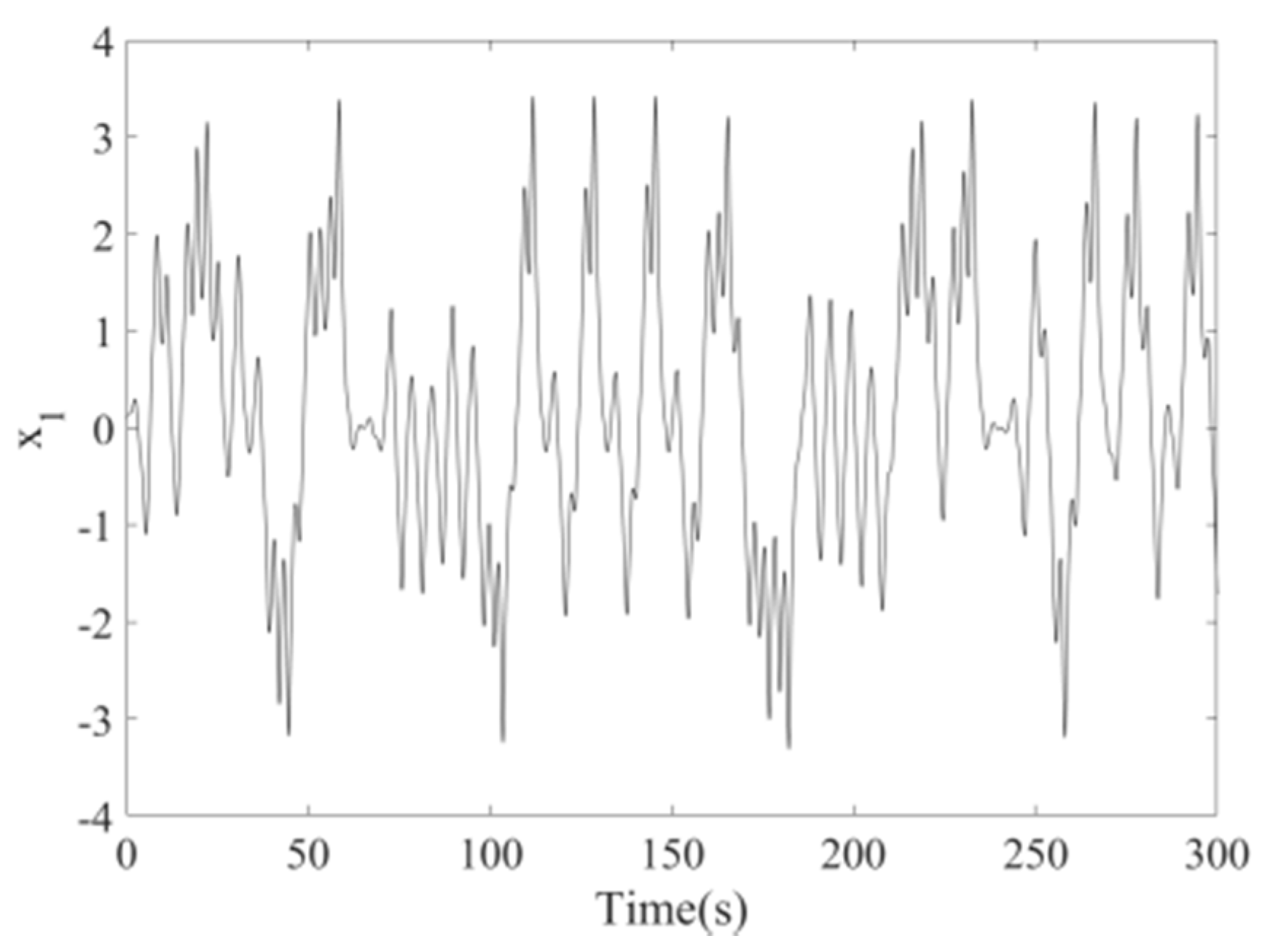
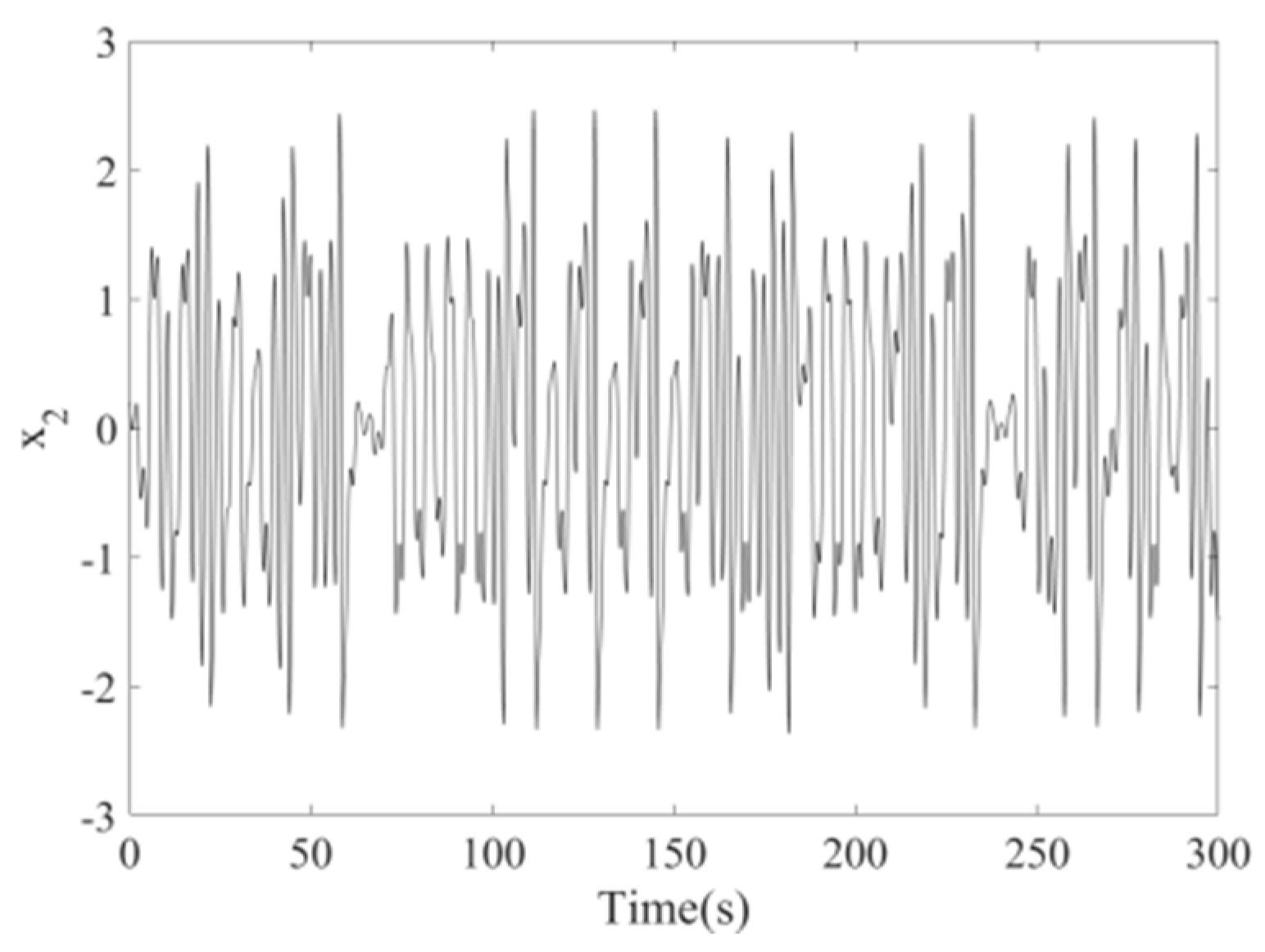
The parametric excitation roll system of a ship is a chaos system that can be proved by MATLAB simulation results. The history charts of
and
of the parametric excitation roll system of the ship are shown in
Figure 1 and
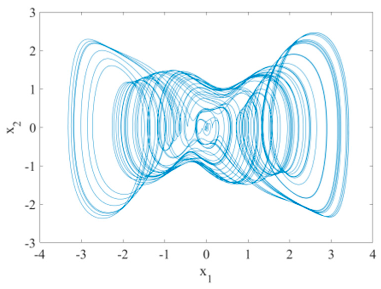
Figure 2, respectively, in which it is clear that the system is in chaos. The phase diagram of the parametric excitation roll system of the ship is shown in
Figure 3, which further proves that the system is a chaos system and similar to a Duffing chaos system.
In the traditional methods,
and
are usually chosen as unknown parameters. In the model
,
is parameter excitation amplitude and
is parameter excitation frequency, which can affect the chaotic state of the system. This method can be seen in references [
24] and [
25].
In the method discussed in this paper, a ship’s parametric excitation rolling system is regarded as a master system. The controller’s chaotic system with unknown parameters independent of the system model is regarded as a slave system. The master system and slave system are based on the ship parametric excitation rolling system with the same fundamental structure. In other words, the chaotic control is achieved over the same structure systems.
Using Equation
, the sliding mode surface is designed as follows:
According to Equation
, the controller with unknown parameters independent of the system is designed as:
From Equation
, the adaptive law of unknown parameters is:
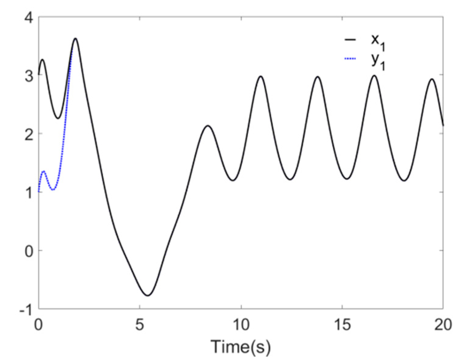
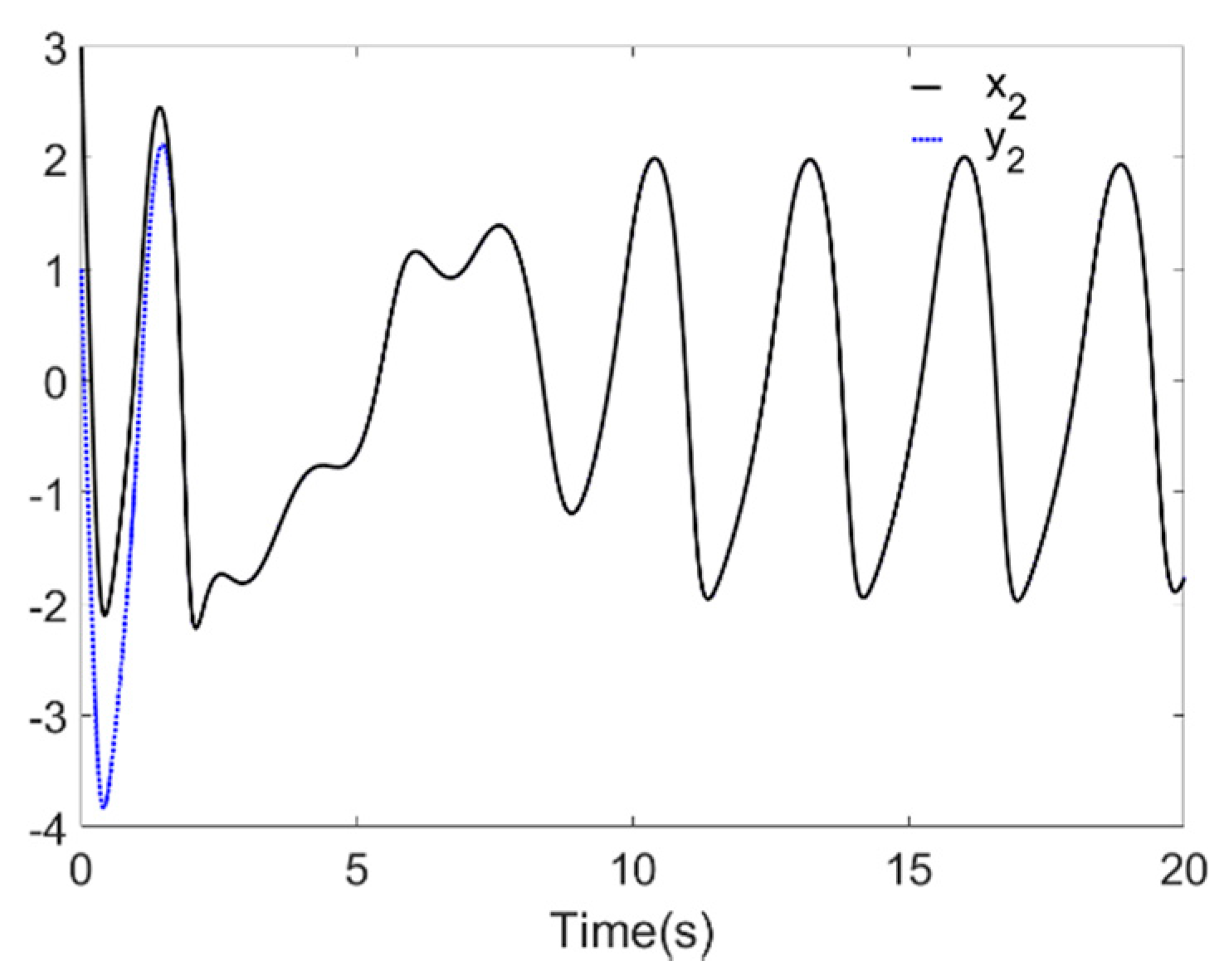
In the simulation, the step size was set to 0.01 s, and the initial values were and . In addition, the initial values of unknown parameters were set to and .
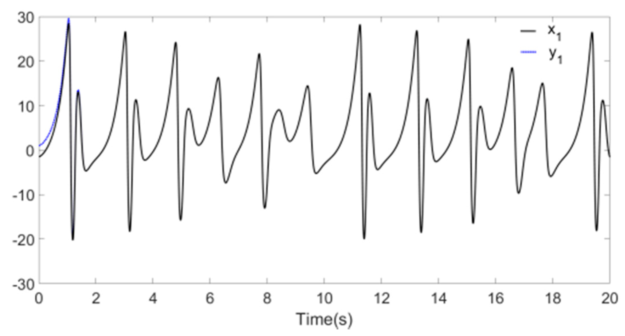
Figure 4 and
Figure 5 reflect the synchronization process of Systems
and
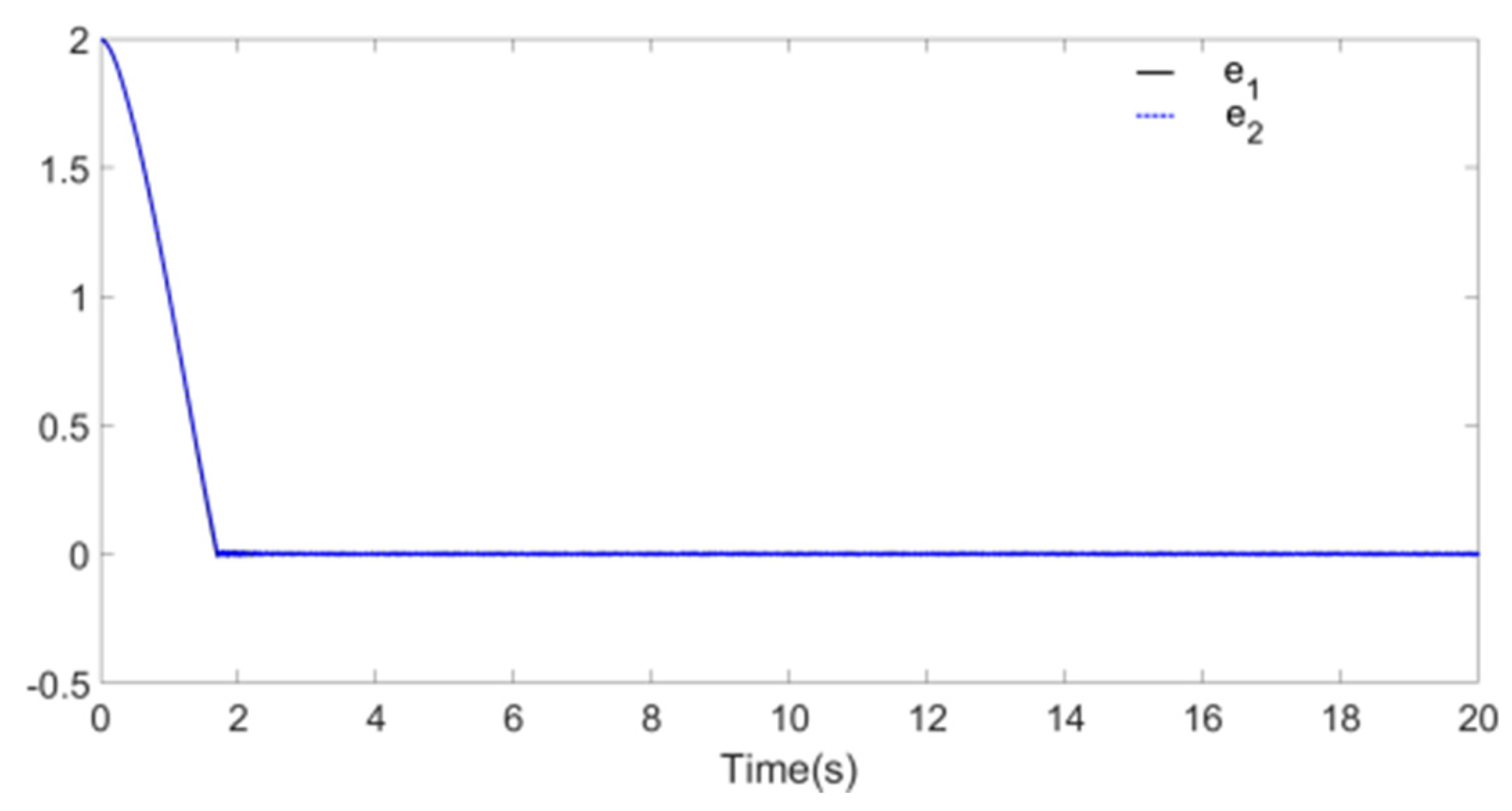
, and synchronization error is shown in
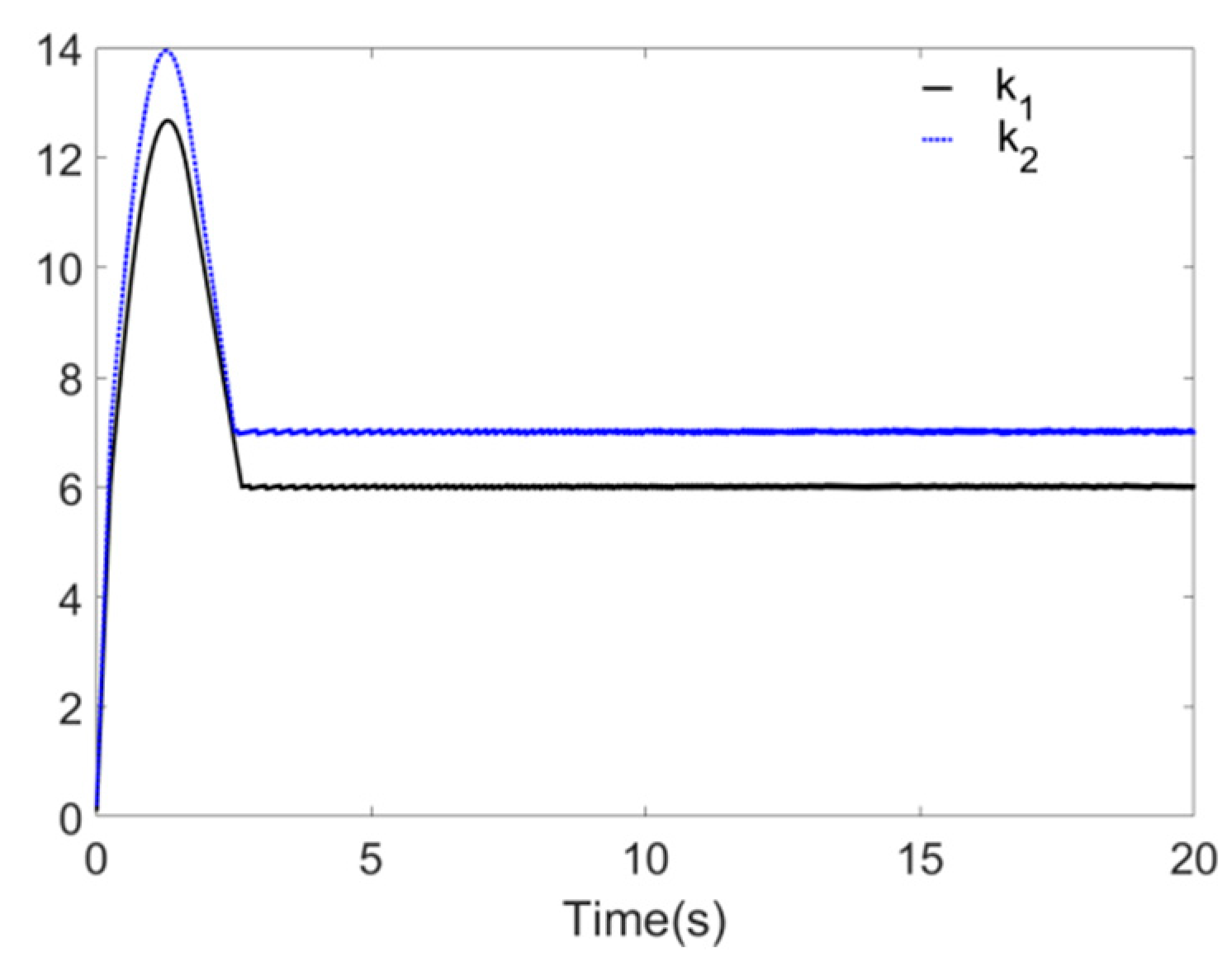
Figure 6, the identification processes of unknown parameters
and
are shown in
Figure 7.
Figure 4 and
Figure 5 demonstrate that, when
t approaches 2 s, the drive system parameters (
and
) synchronize with the response system parameters (
and
). The error effect in
Figure 6 shows that, when
t approaches 2 s, errors
and
stabilize around zero. Finally,
Figure 7 demonstrates that, when
t approaches 2 s, the parameters
and
reach values 6 and 7, respectively.
By using the parameters to update the rule , one can identify the special unknown parameters in the controller . In other words, the drive system and the response system reach a finite-time synchronization. After the controller facilitates the ship parametric excitation rolling system with unknown parameters independent of the system model, the response system successfully tracks the original system in a finite time. The adaptive parameters converge to bounded values within the finite time.
4.2. Simulation Verification of Chaotic System with Different Structures
Both the Liu system and the Lorenz system [
31,
32] are well-known chaotic systems that do not require a detailed introduction. In addition, their structures are different. In the traditional methods, the coefficients of the equations are usually chosen as unknown parameters. The coefficients of these equations can affect the chaotic state of the system. This treatment method can be seen in references [
24,
25].
Here, the method mentioned in the previous section are used to verify the proposed method’s performance in the chaotic synchronization of systems with different structures.
Using the Equation
, the sliding mode surface is designed as follows:
According to Equation
, the controller with unknown parameters independent of the system is designed as:
From Equation
, the adaptive law of unknown parameters is:
In the simulation, the step size was set to 0.01 s, and the initial values were ,, and . In addition, the initial values of unknown parameters were set to .
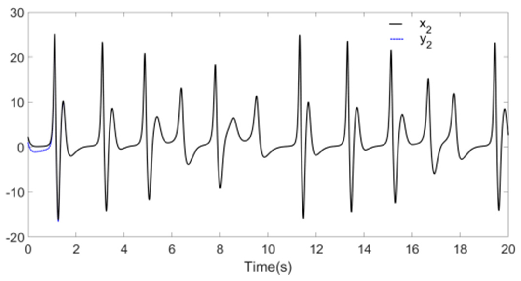
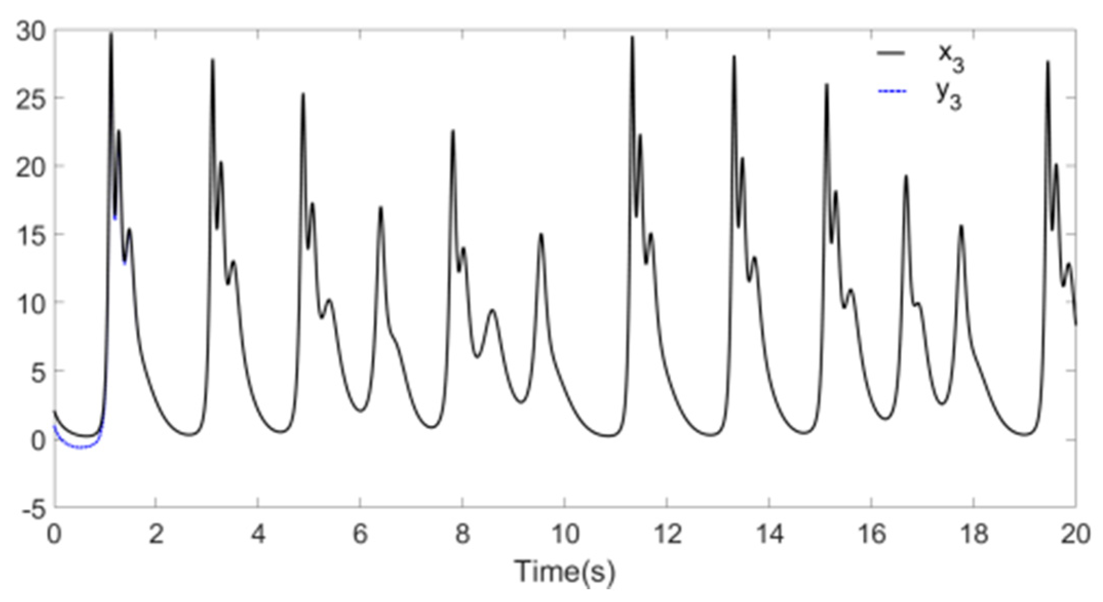
Figure 8,
Figure 9 and
Figure 10 reflect the synchronization process of Systems
and
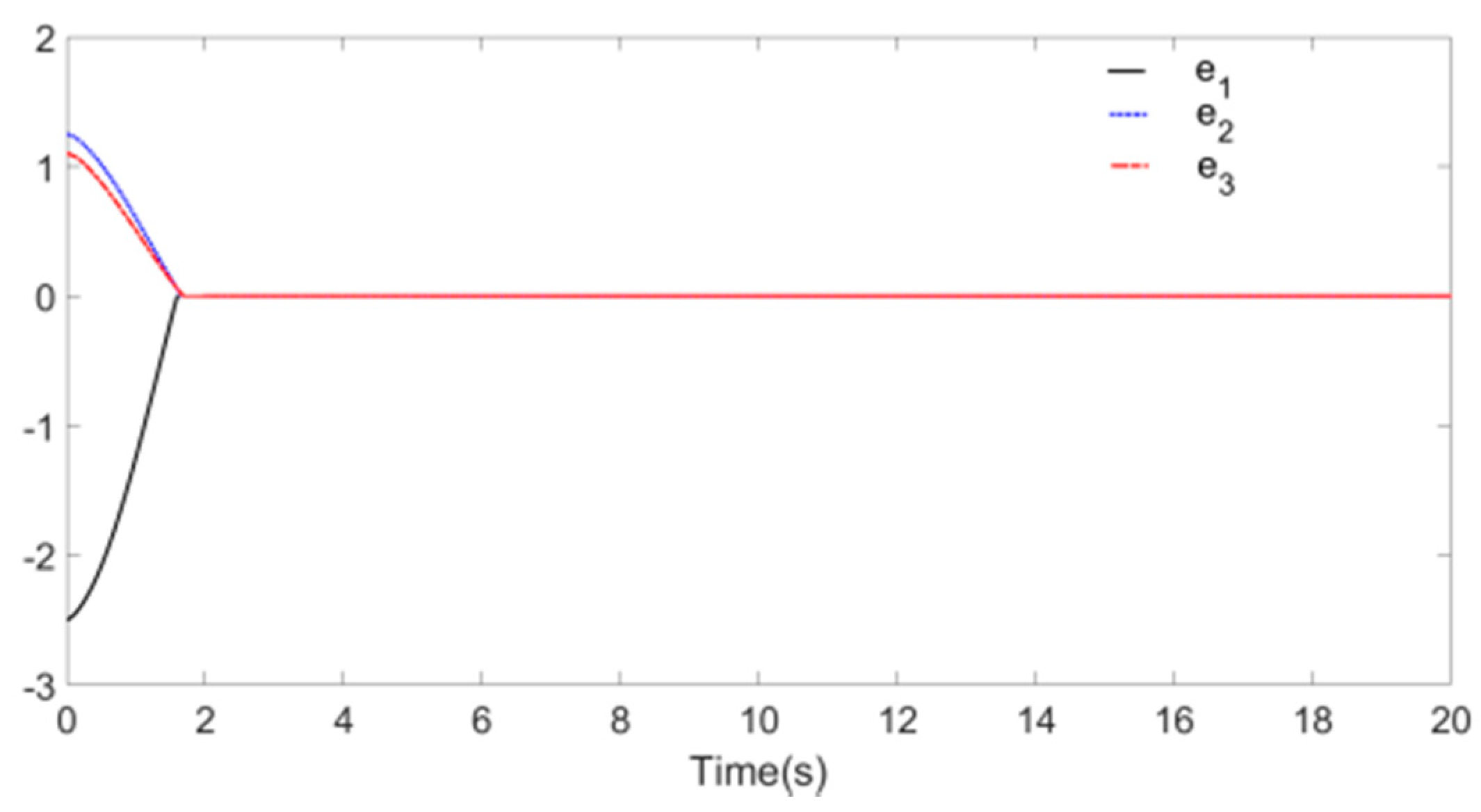
, and synchronization error is shown in
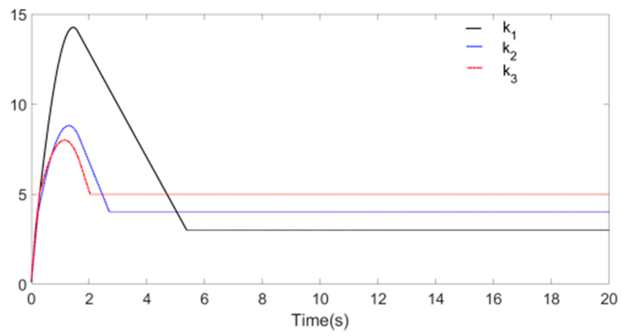
Figure 11, the identification processes of unknown parameters
are shown in
Figure 12.
Figure 8,
Figure 9 and
Figure 10 demonstrate that, when
t approaches 1.7 s, the drive system parameters (
,
and
) synchronize with the response system parameters (
,
and
). The error effect in
Figure 11 shows that, when
t approaches 1.7 s, errors
,
, and
stabilize around zero. Finally,
Figure 12 demonstrates that, when
t approaches 1.7 s, the parameters
,
, and
reach values 5.2, 2.5, and 2, respectively.
By using the parameters to update the rule , one can identify the special unknown parameters in the controller . In other words, the master system and the slave system reach a finite-time synchronization. The adaptive parameters converge to bounded values within the finite time. The effectiveness of the algorithm is further proved.


