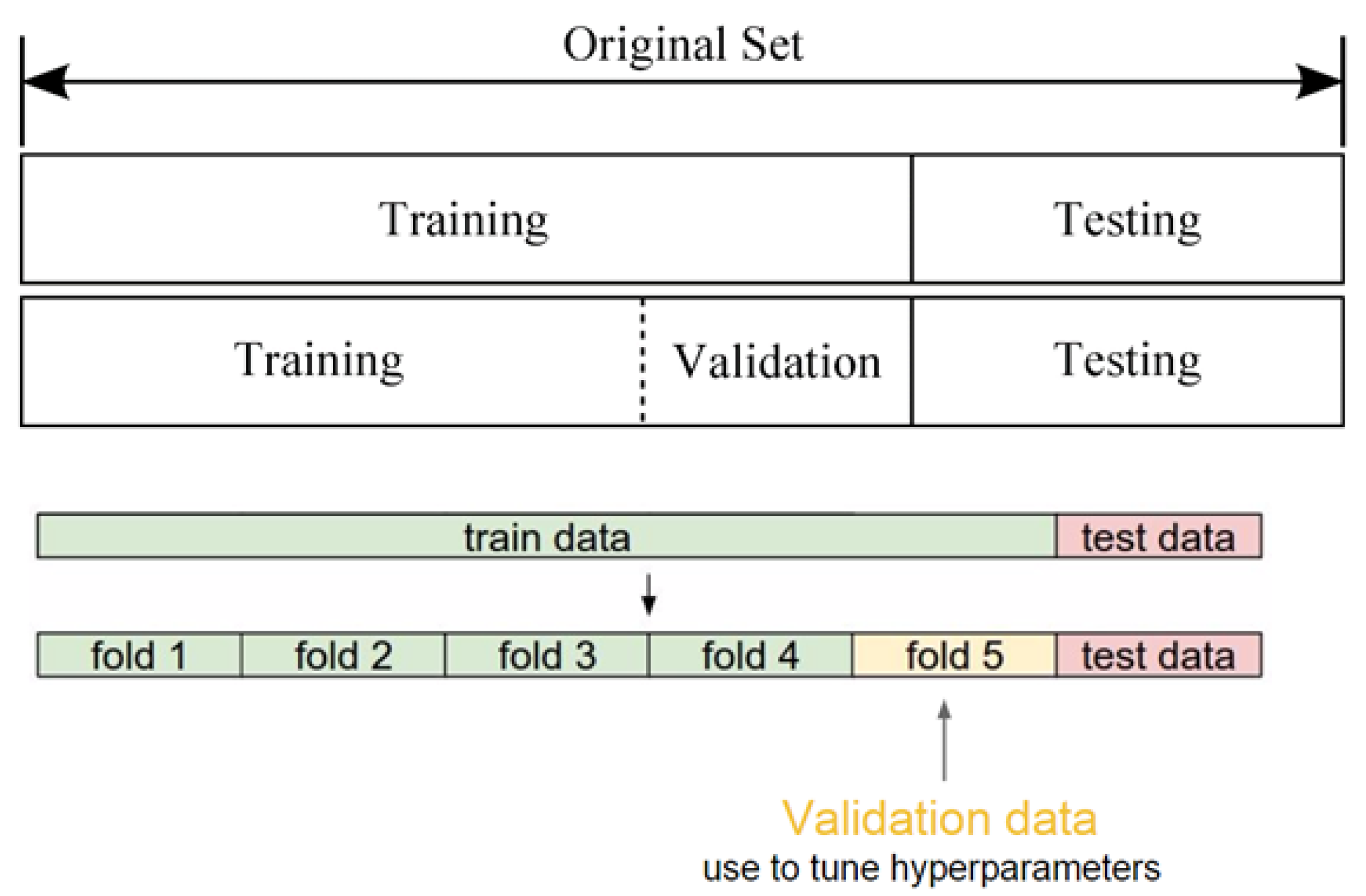
Figure 1.
K-fold cross-validation process.
Figure 1.
K-fold cross-validation process.
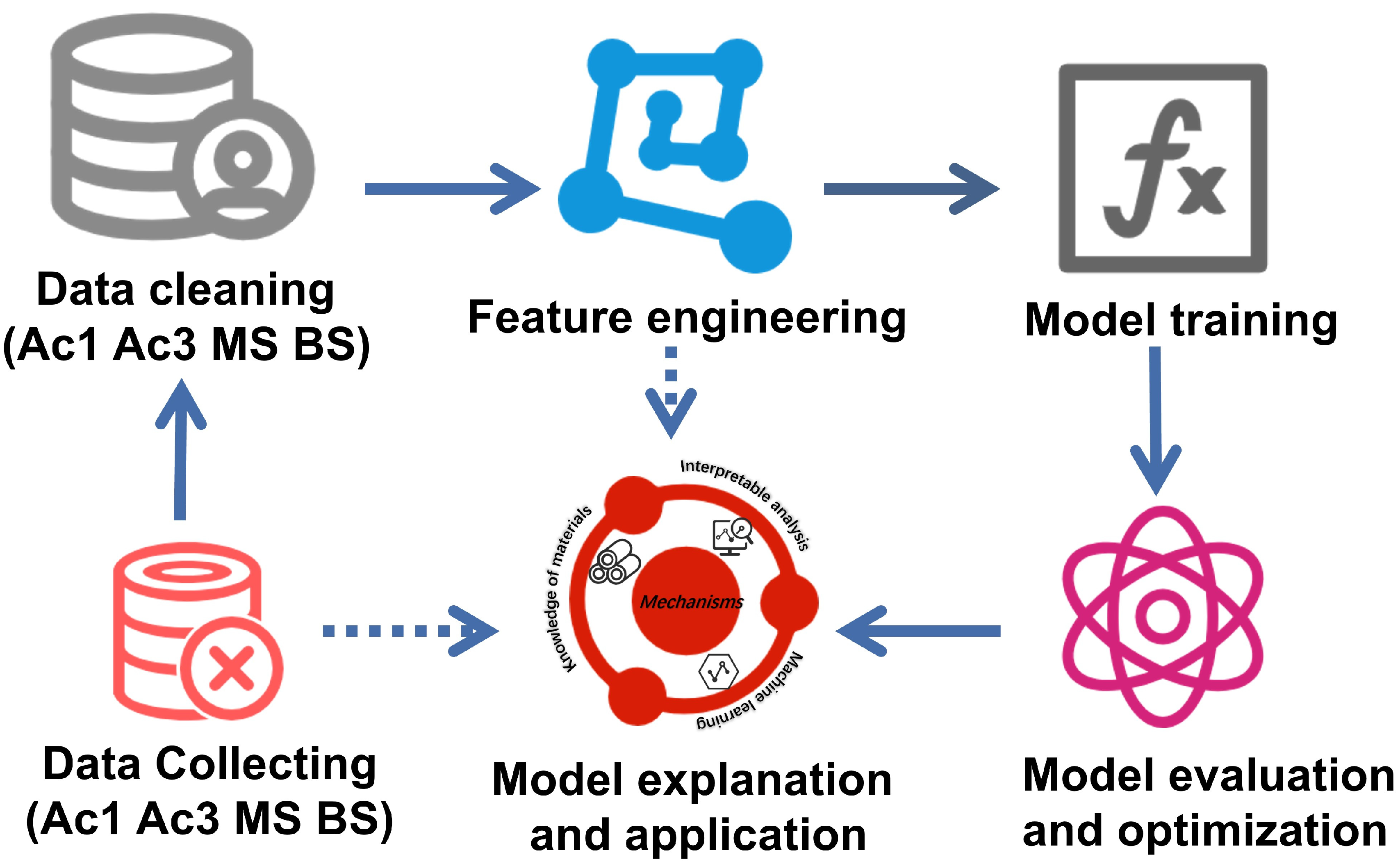
Figure 2.
The workflow of the present work.
Figure 2.
The workflow of the present work.
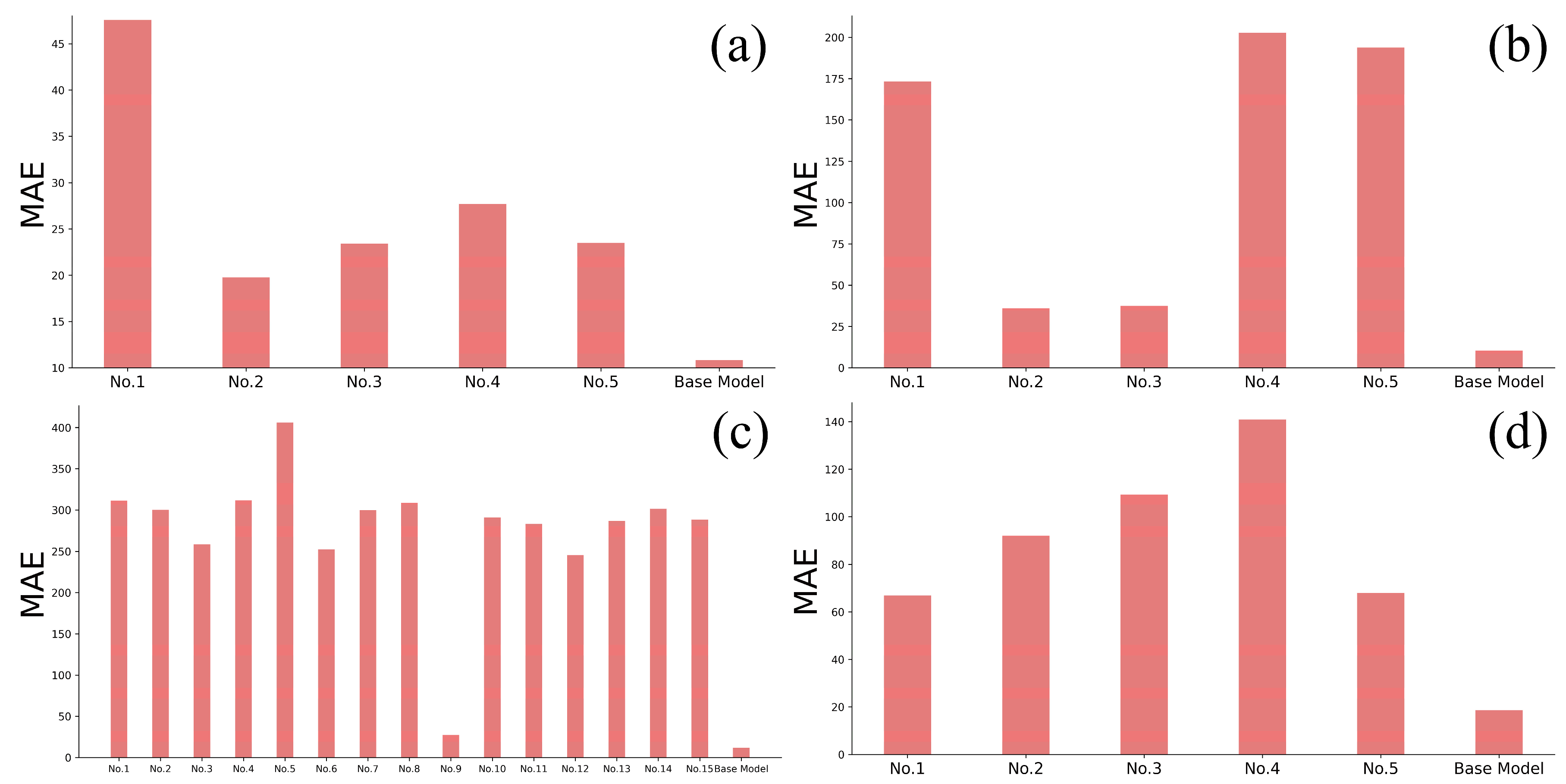
Figure 3.
Comparison between the performance of the empirical formulations and trained machine learning models without atomic parameters. (a) Ac1, (b) Ac3, (c) MS and (d) BS.
Figure 3.
Comparison between the performance of the empirical formulations and trained machine learning models without atomic parameters. (a) Ac1, (b) Ac3, (c) MS and (d) BS.
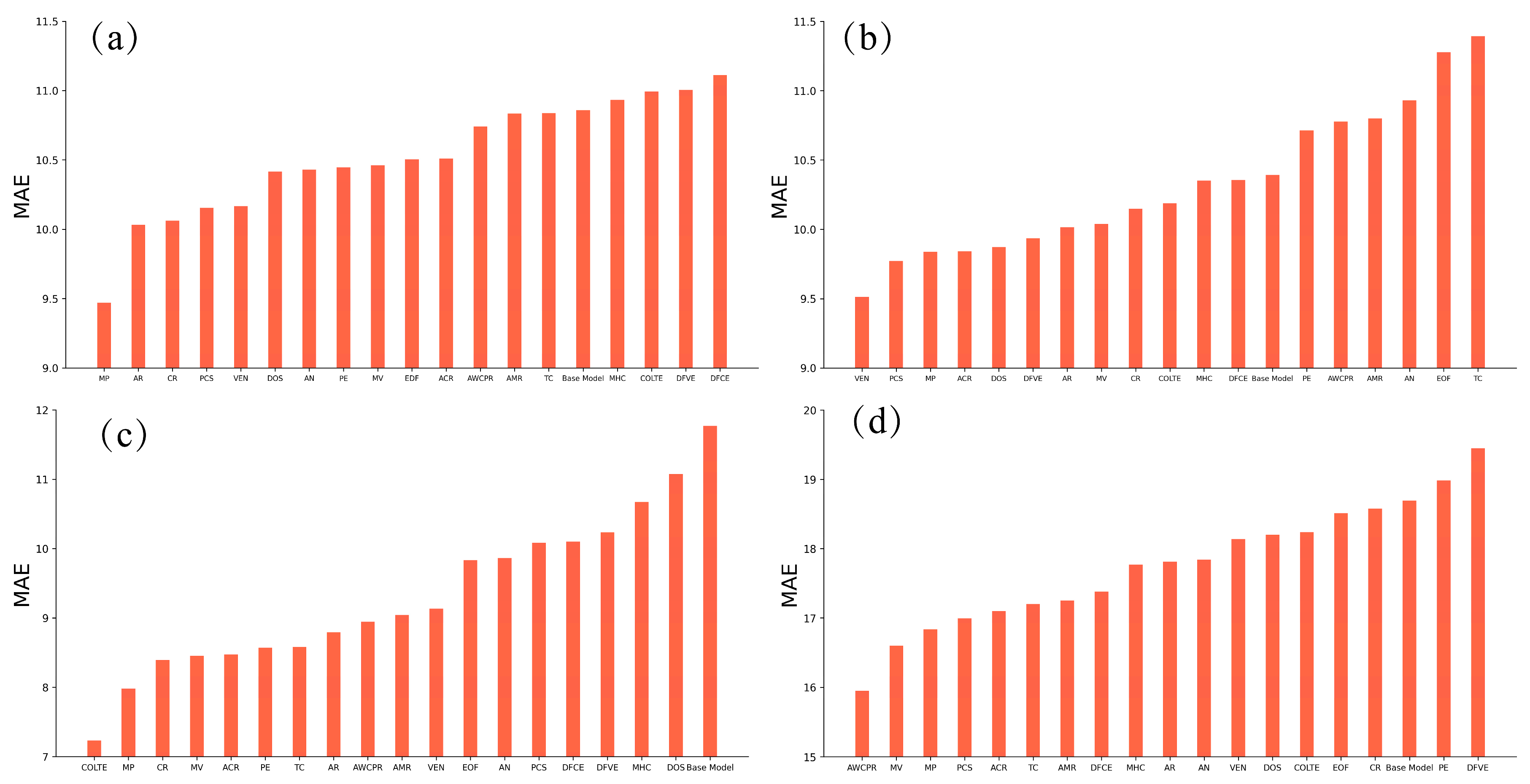
Figure 4.
MAE of the trained models by machine learning with atomic parameters. (a) Ac1, (b) Ac3, (c) MS and (d) BS.
Figure 4.
MAE of the trained models by machine learning with atomic parameters. (a) Ac1, (b) Ac3, (c) MS and (d) BS.
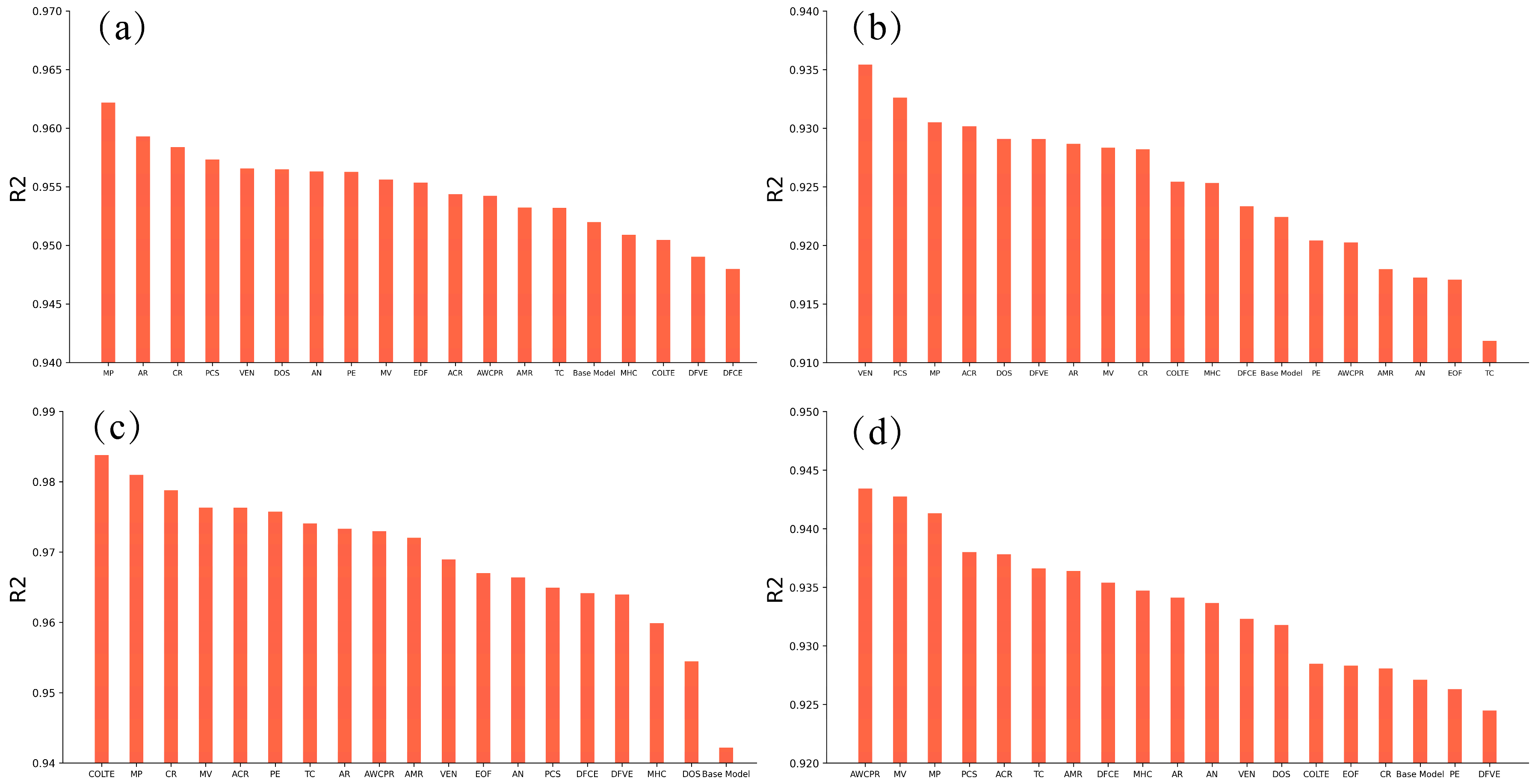
Figure 5.
R2 of the trained models by machine learning with atomic parameters. (a) Ac1, (b) Ac3, (c) MS and (d) BS.
Figure 5.
R2 of the trained models by machine learning with atomic parameters. (a) Ac1, (b) Ac3, (c) MS and (d) BS.
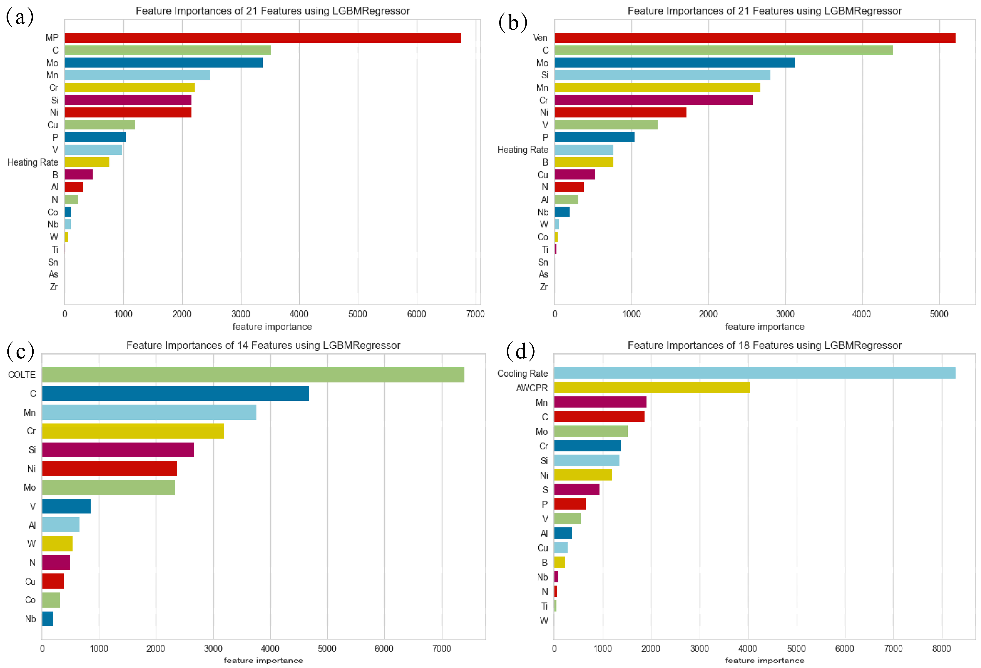
Figure 6.
Feature importance analysis in the training process. (a) Ac1, (b) Ac3, (c) MS and (d) BS.
Figure 6.
Feature importance analysis in the training process. (a) Ac1, (b) Ac3, (c) MS and (d) BS.
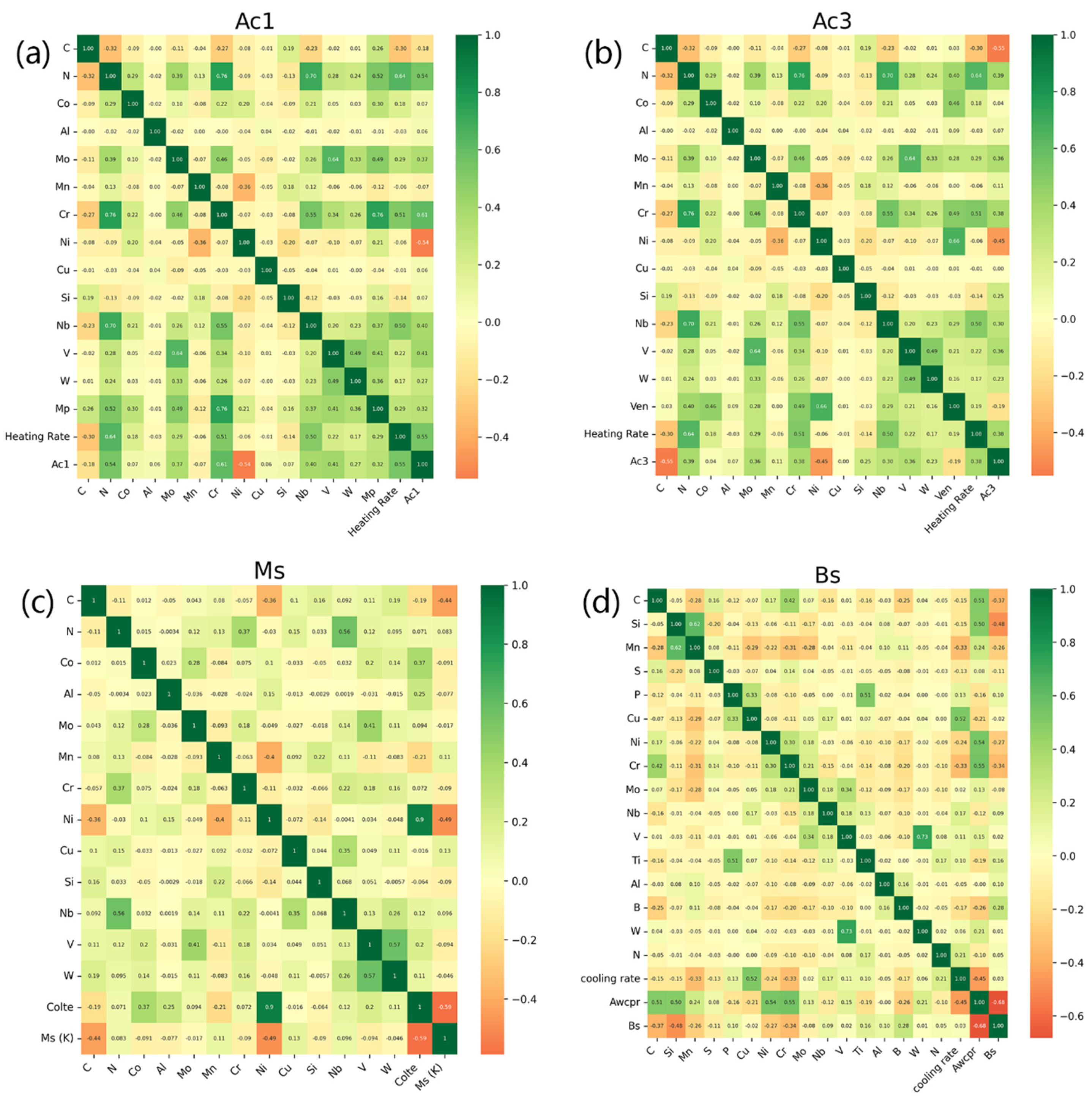
Figure 7.
Feature correlation heatmap between the features and the specific phase transformation temperature. (a) Ac1, (b) Ac3, (c) MS and (d) BS.
Figure 7.
Feature correlation heatmap between the features and the specific phase transformation temperature. (a) Ac1, (b) Ac3, (c) MS and (d) BS.
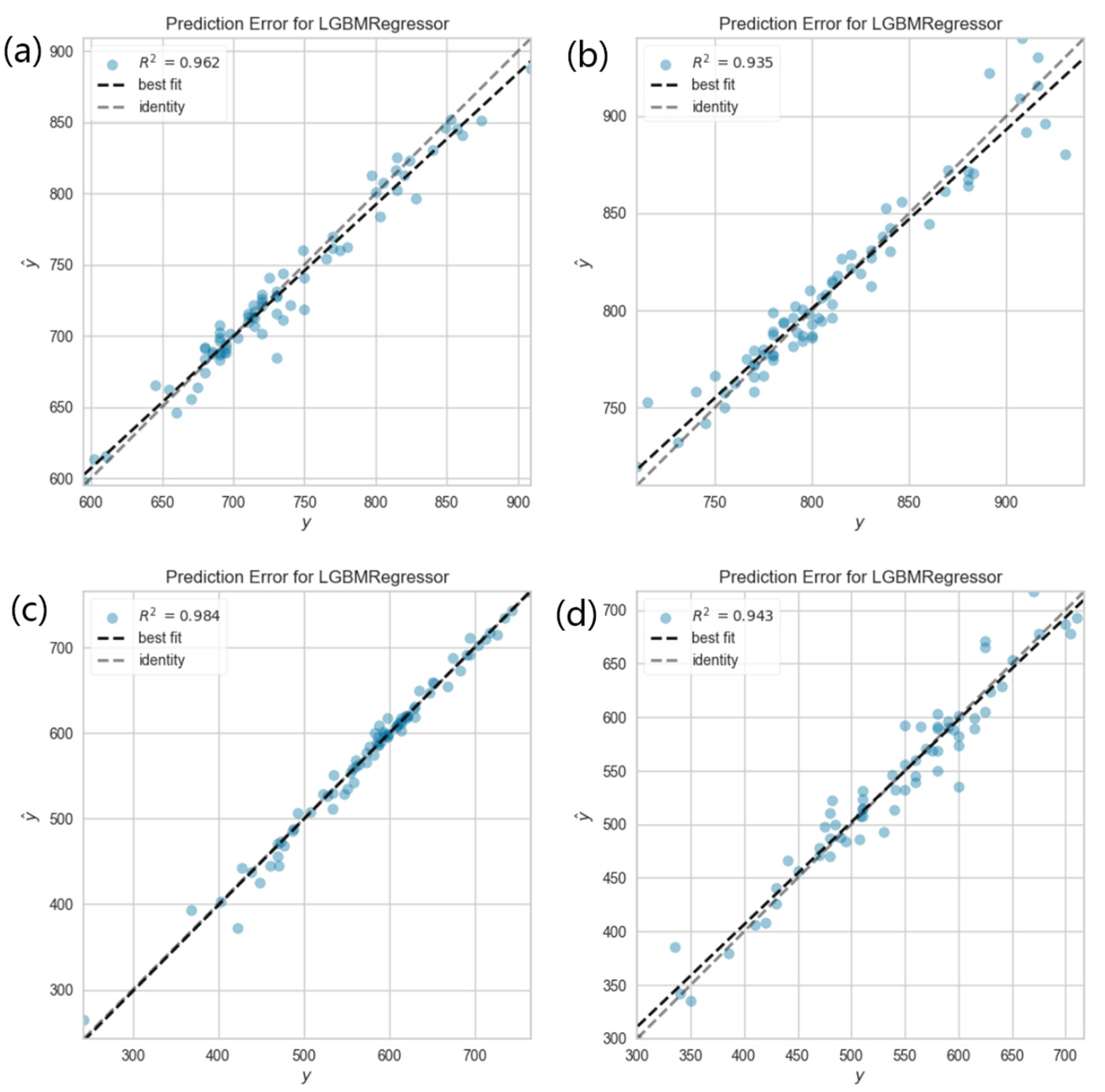
Figure 8.
The fitting results in the models with the best atomic parameters. (a) Ac1, (b) Ac3, (c) MS and (d) BS.
Figure 8.
The fitting results in the models with the best atomic parameters. (a) Ac1, (b) Ac3, (c) MS and (d) BS.
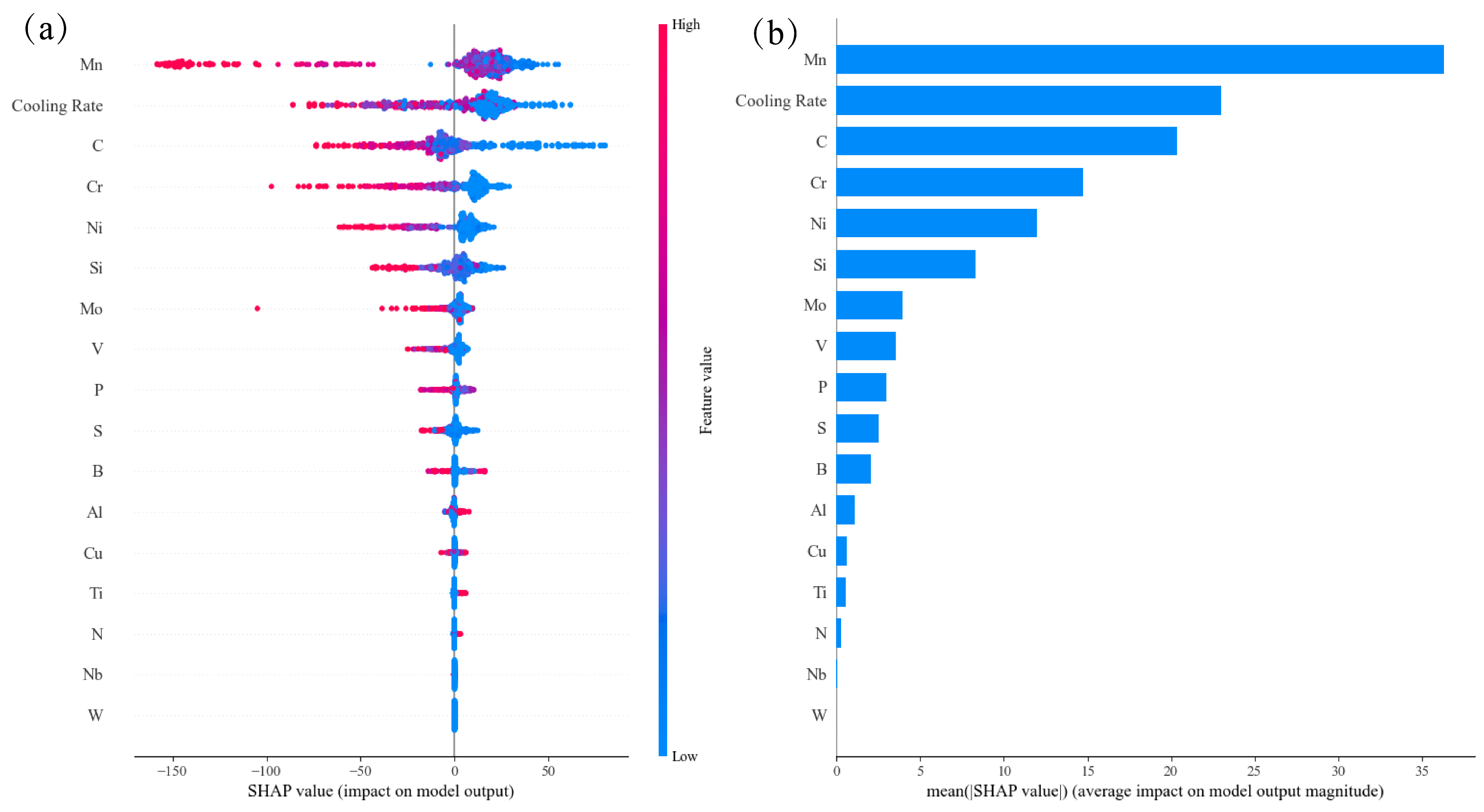
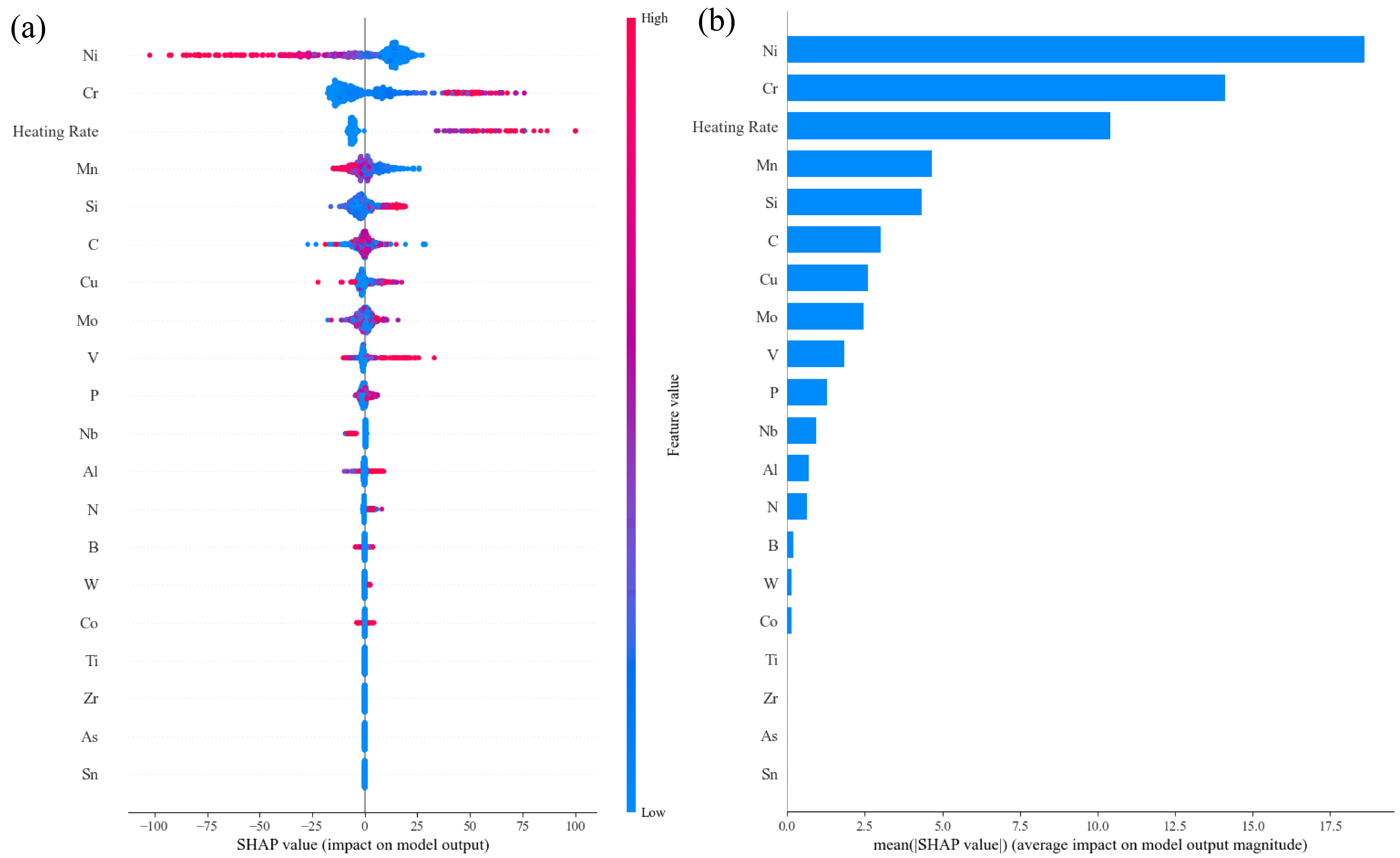
Figure 9.
SHAP analysis in the trained MS prediction model: (a) impact on model output and (b) average impact on model output magnitude.
Figure 9.
SHAP analysis in the trained MS prediction model: (a) impact on model output and (b) average impact on model output magnitude.
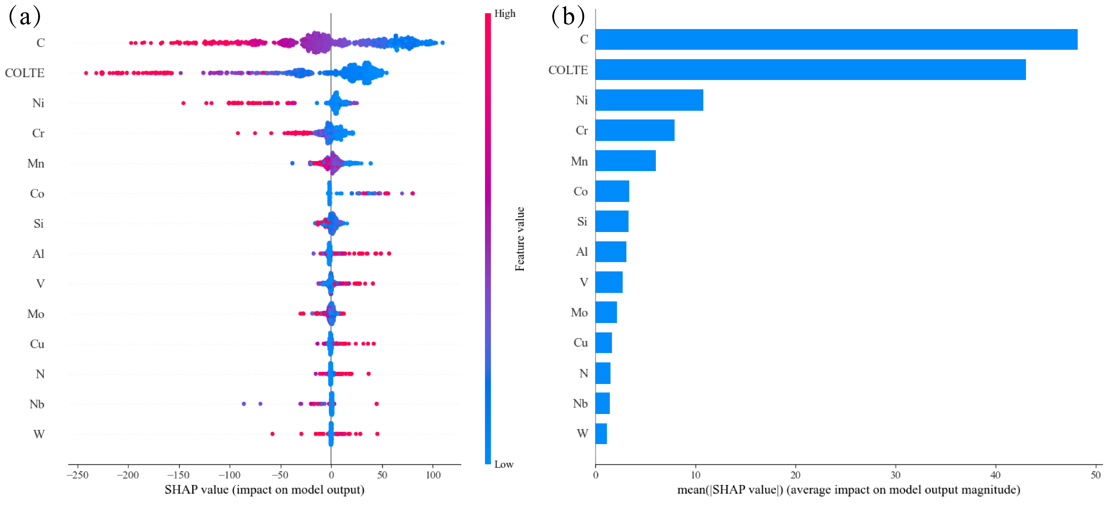
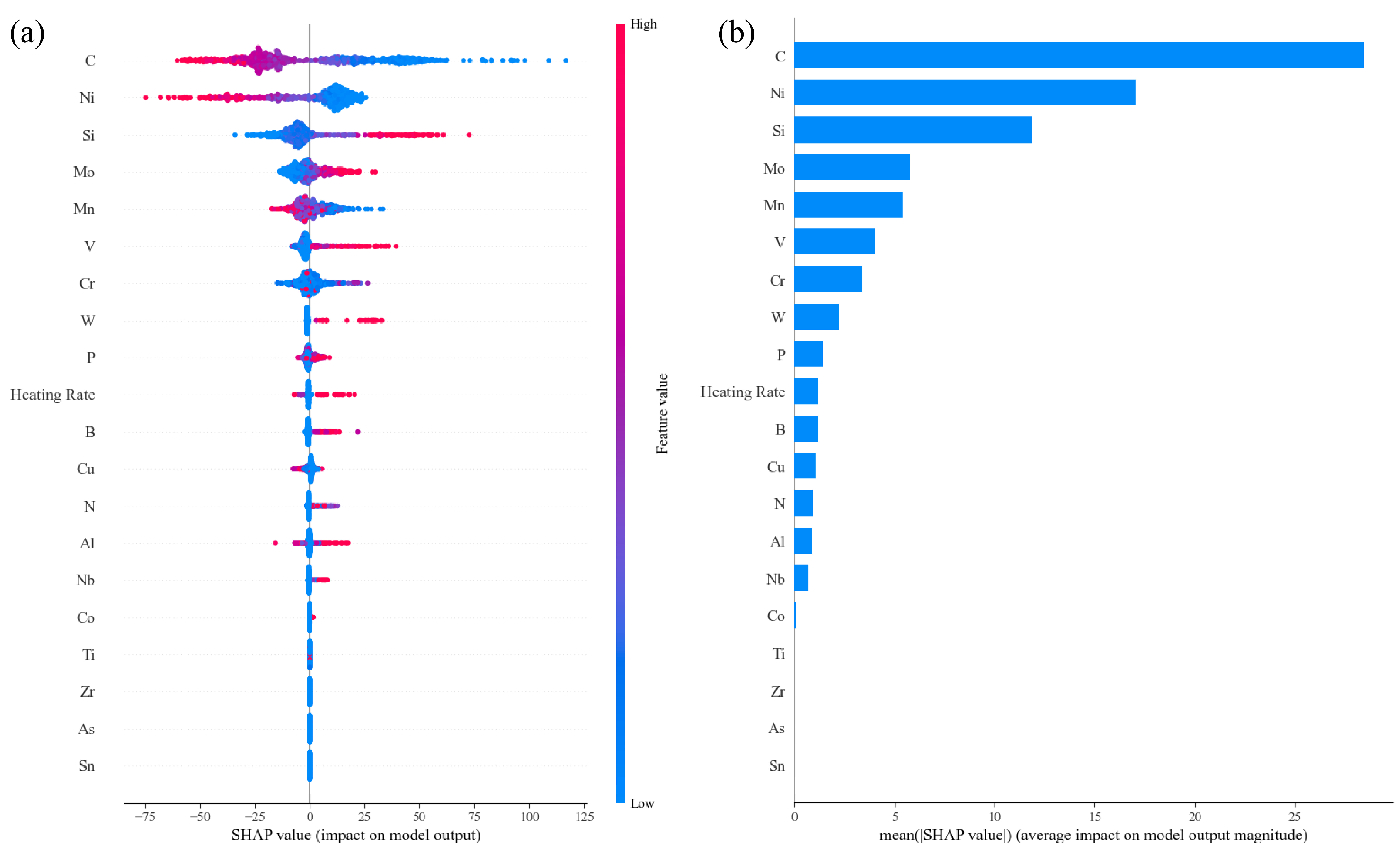
Figure 10.
SHAP analysis in the trained BS prediction model: (a) impact on model output and (b) average impact on model output magnitude.
Figure 10.
SHAP analysis in the trained BS prediction model: (a) impact on model output and (b) average impact on model output magnitude.
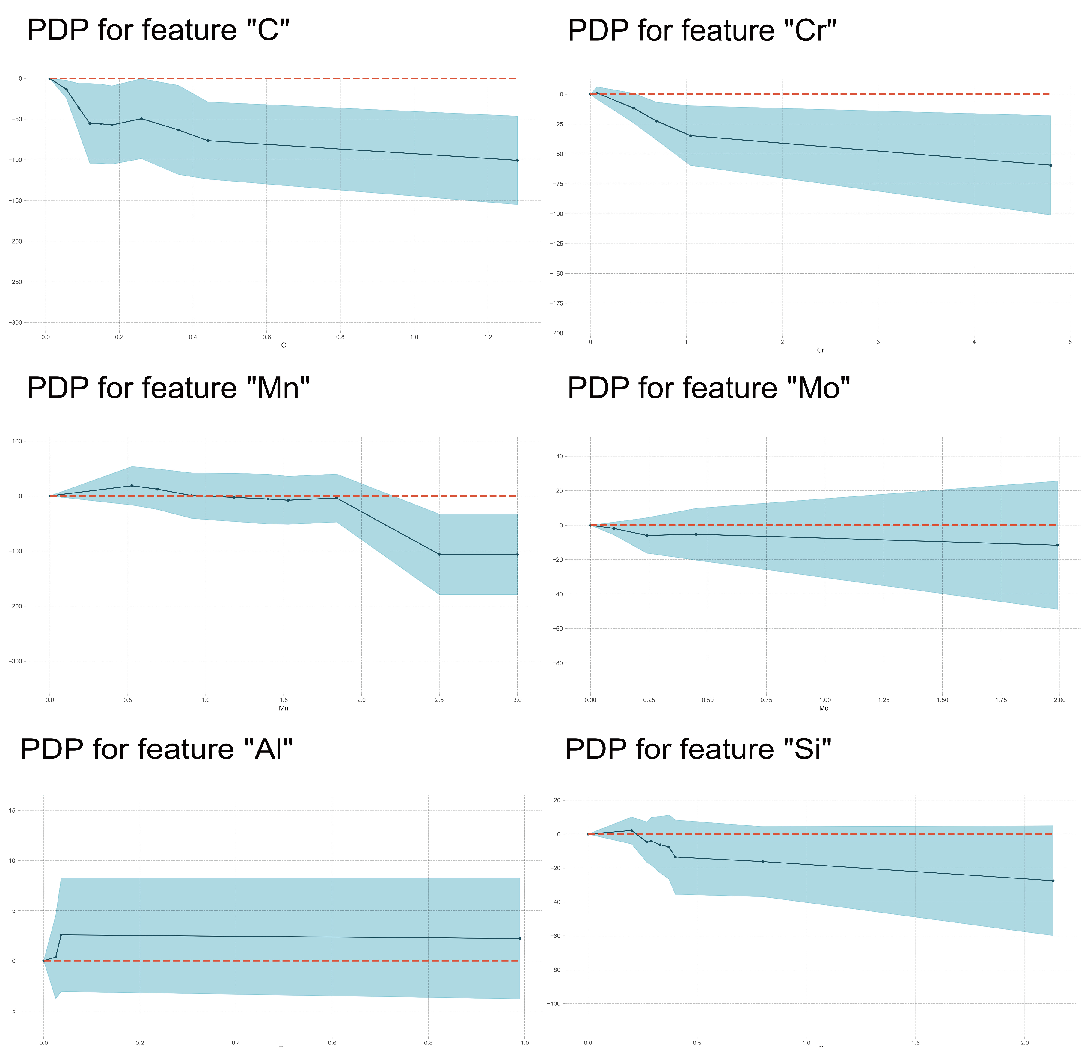
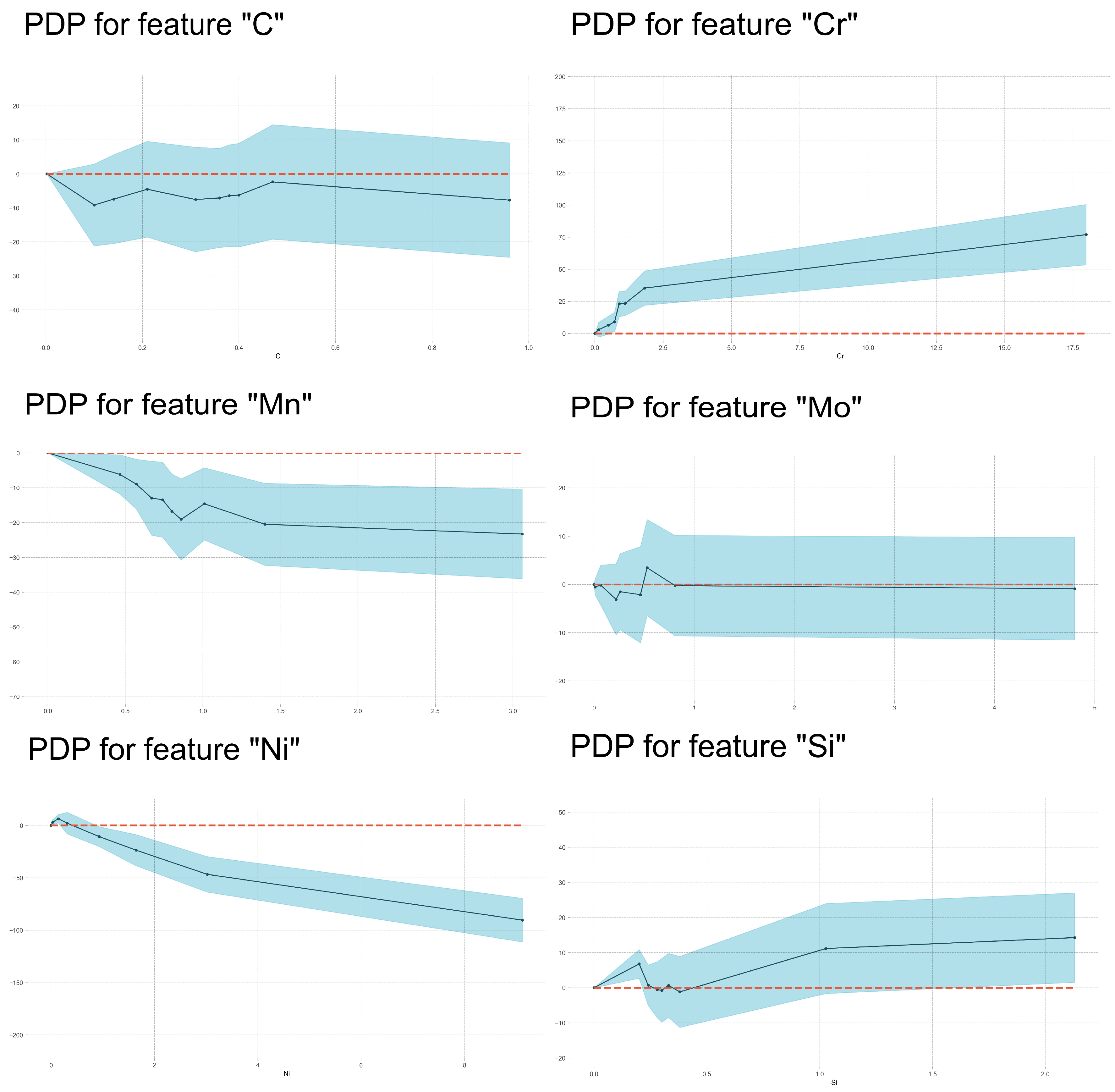
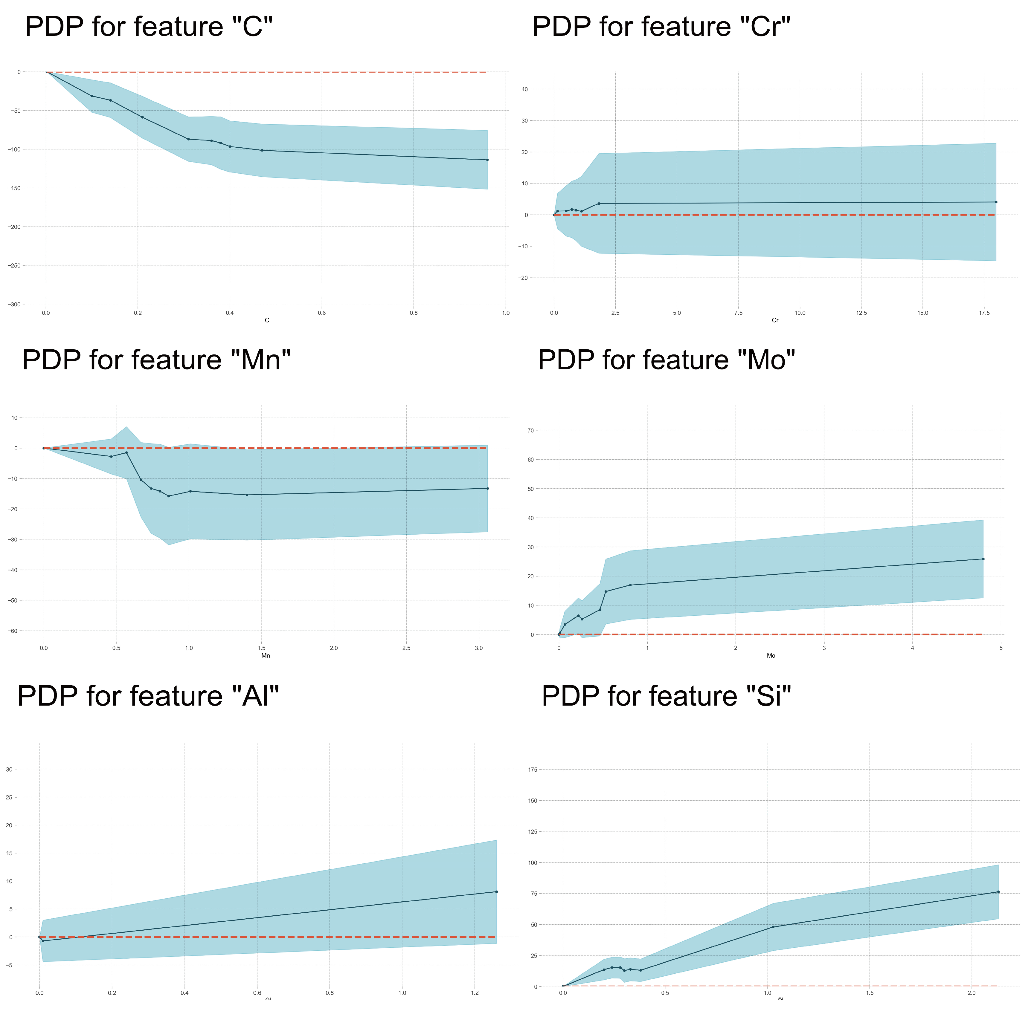
Figure 11.
PDP analysis on the effects of alloying element content on BS temperature.
Figure 11.
PDP analysis on the effects of alloying element content on BS temperature.
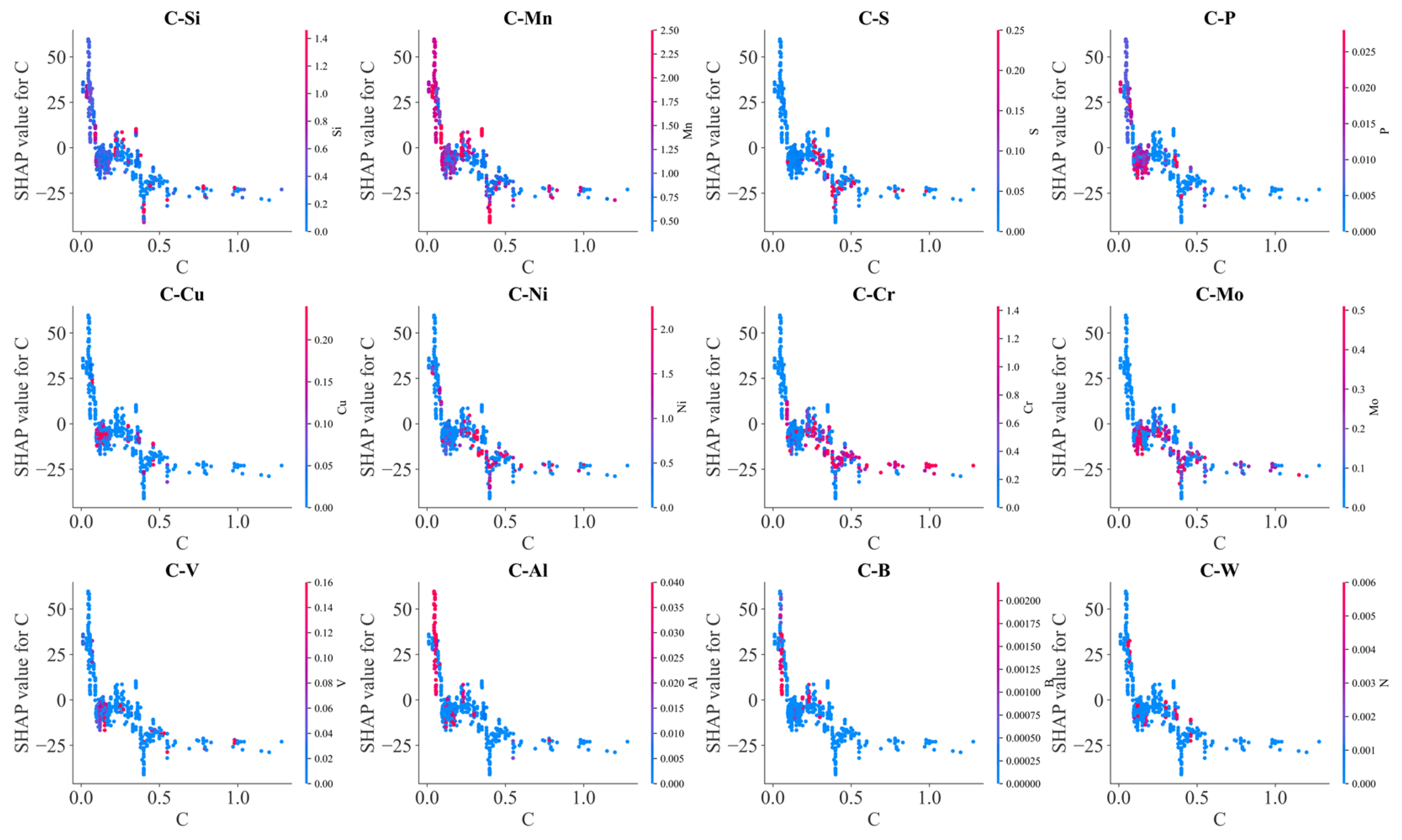
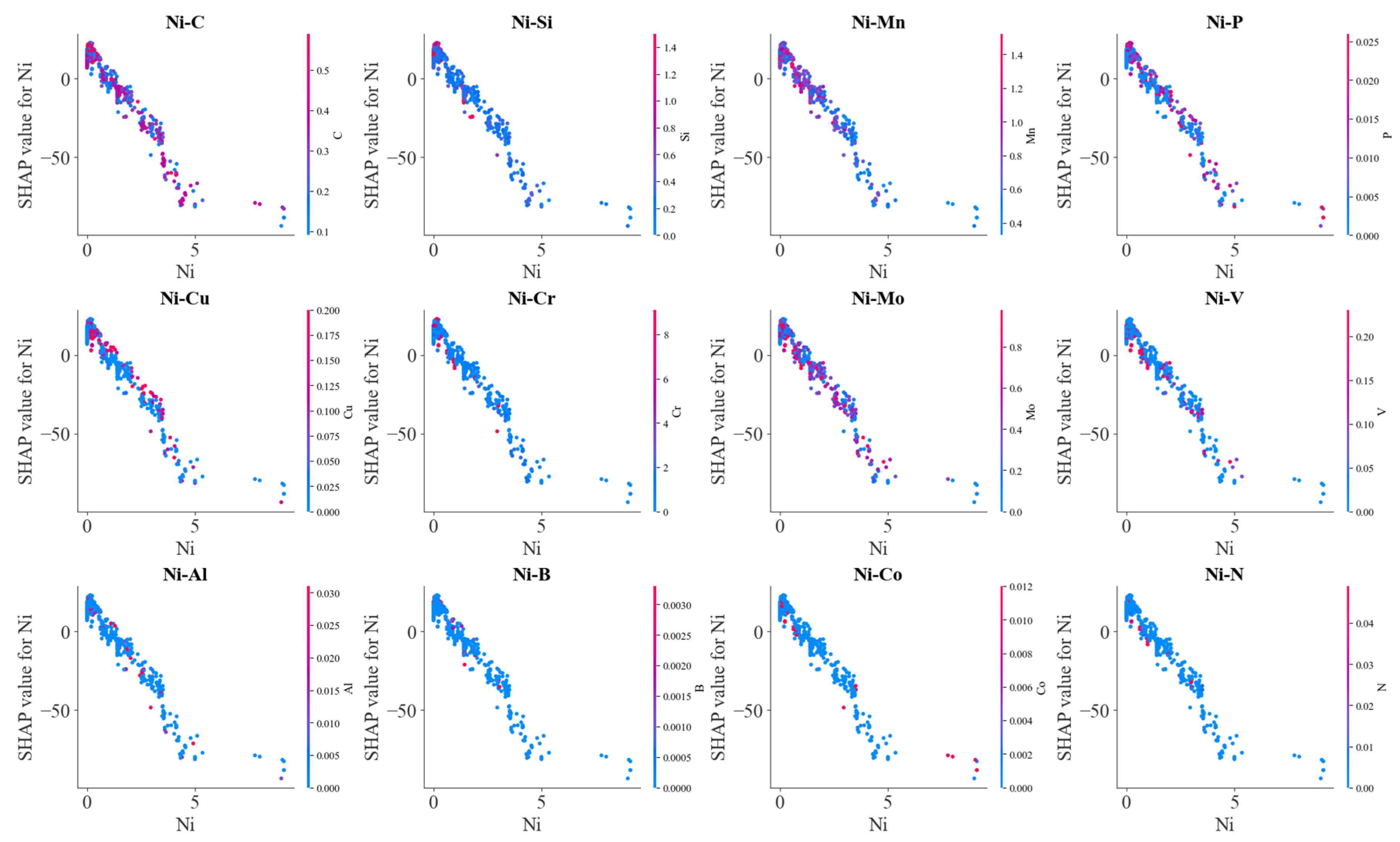
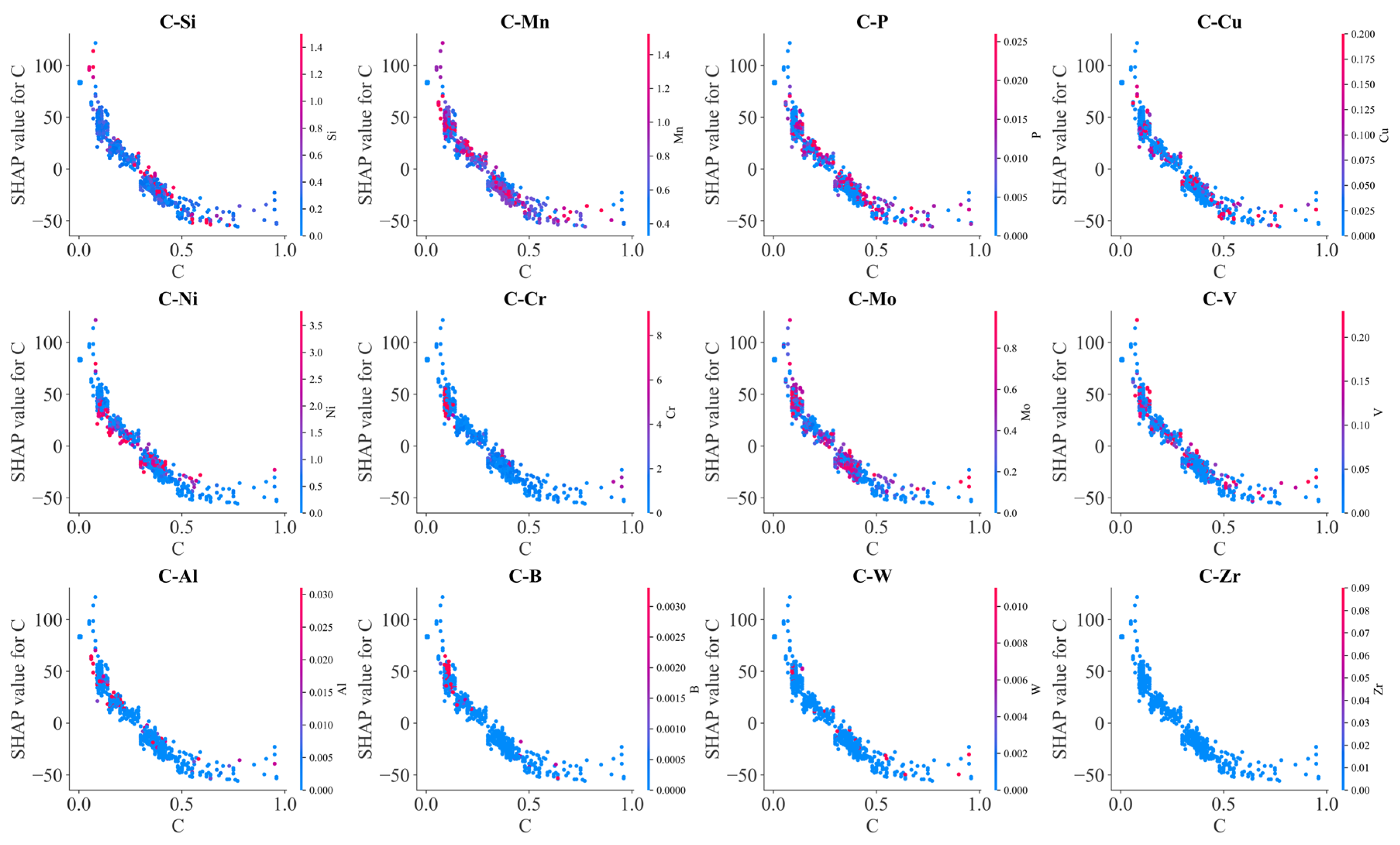
Figure 12.
SHAP analysis on the effects of alloy element C on BS temperature.
Figure 12.
SHAP analysis on the effects of alloy element C on BS temperature.
Figure 13.
SHAP analysis in the trained Ac1 prediction model: (a) impact on model output and (b) average impact on model output magnitude.
Figure 13.
SHAP analysis in the trained Ac1 prediction model: (a) impact on model output and (b) average impact on model output magnitude.
Figure 14.
PDP analysis on the effects of alloying element content on Ac1 temperature.
Figure 14.
PDP analysis on the effects of alloying element content on Ac1 temperature.
Figure 15.
SHAP analysis on the effects of alloy element Ni on Ac1 temperature.
Figure 15.
SHAP analysis on the effects of alloy element Ni on Ac1 temperature.
Figure 16.
SHAP analysis in the trained Ac3 prediction model: (a) impact on model output and (b) average impact on model output magnitude.
Figure 16.
SHAP analysis in the trained Ac3 prediction model: (a) impact on model output and (b) average impact on model output magnitude.
Figure 17.
PDP analysis on the effects of alloying element content on Ac3 temperature.
Figure 17.
PDP analysis on the effects of alloying element content on Ac3 temperature.
Figure 18.
SHAP analysis on the effects of alloy element C on Ac3 temperature.
Figure 18.
SHAP analysis on the effects of alloy element C on Ac3 temperature.
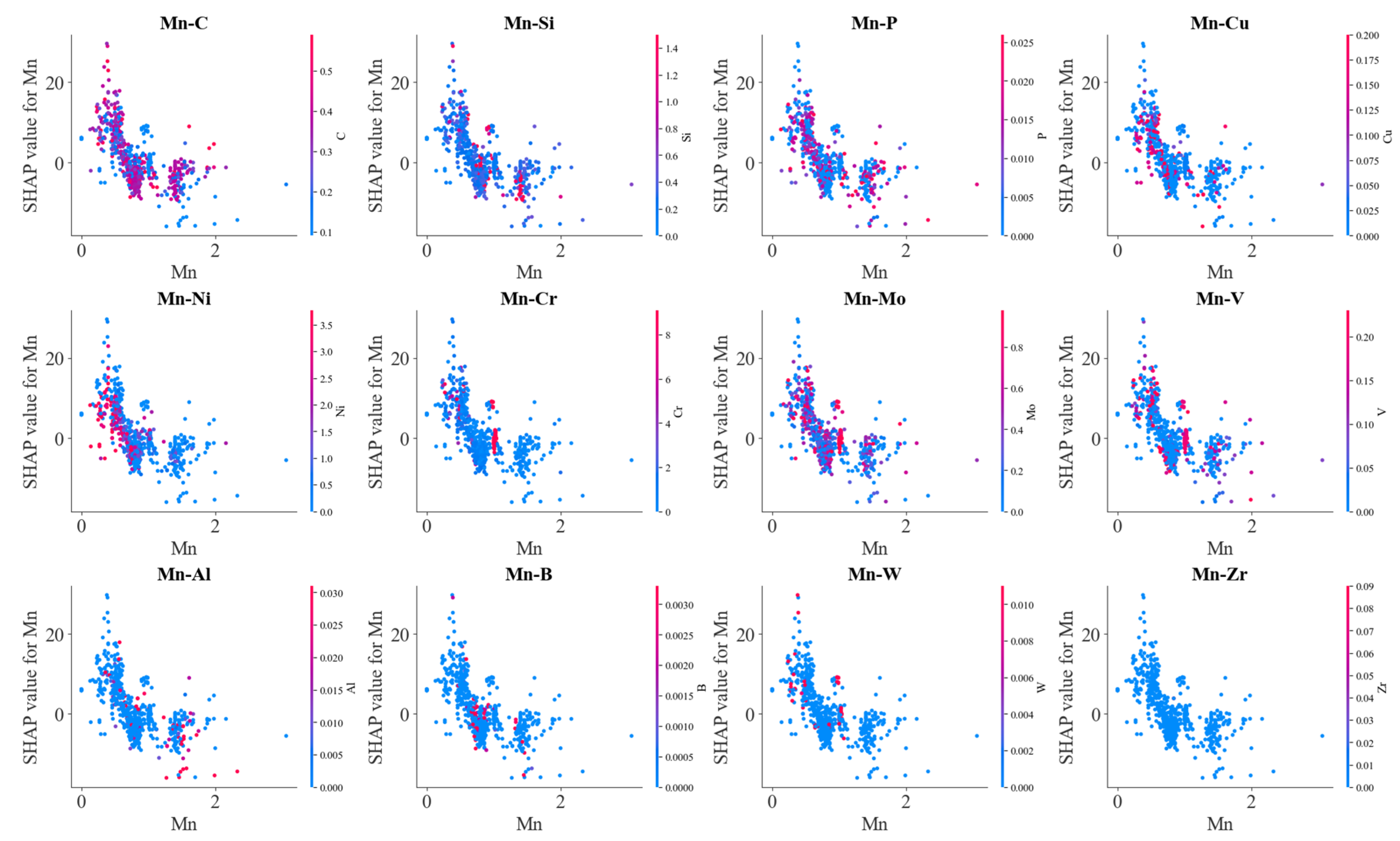
Figure 19.
SHAP analysis on the effects of alloy element Mn on Ac3 temperature.
Figure 19.
SHAP analysis on the effects of alloy element Mn on Ac3 temperature.
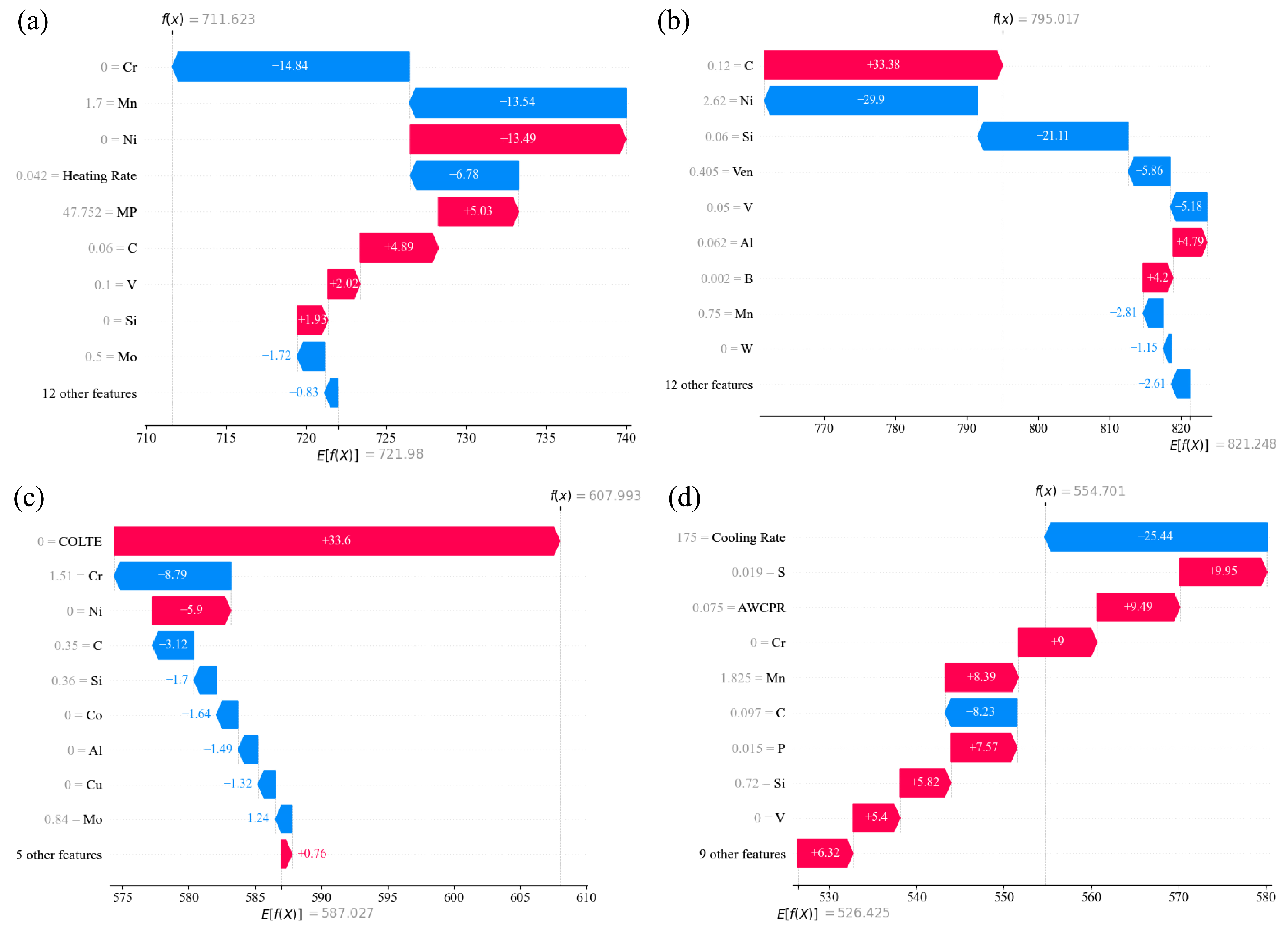
Figure 20.
Examples of model predictions. (a) Ac1 (b) Ac3 (c) MS (d) BS.
Figure 20.
Examples of model predictions. (a) Ac1 (b) Ac3 (c) MS (d) BS.
Table 1.
Dataset size after data cleaning.
Table 1.
Dataset size after data cleaning.
| Dataset | The Sample Size |
|---|
| MS | 800 |
| Ac1 | 735 |
| Ac3 | 735 |
| BS | 655 |
Table 2.
Number of deleted samples.
Table 2.
Number of deleted samples.
| Dataset | Number |
|---|
| MS | 150 |
| Ac1 | 54 |
| Ac3 | 53 |
| BS | 49 |
Table 3.
Overall information of MS dataset.
Table 3.
Overall information of MS dataset.
| Elements | Minimum | Maximum | Mean | Standard Deviation |
|---|
| Carbon (wt.%) | 0.0016 | 1.8 | 0.36 | 0.247 |
| Silicon (wt.%) | 0 | 3.8 | 0.394 | 0.441 |
| Manganese (wt.%) | 0 | 10.24 | 0.867 | 0.801 |
| Sulfur (wt.%) | 0 | 0.054 | 0.003 | 0.007 |
| Phosphorus (wt.%) | 0 | 0.044 | 0.003 | 0.008 |
| Cuprum (wt.%) | 0 | 1.49 | 0.035 | 0.108 |
| Nickel (wt.%) | 0 | 31.3 | 2.026 | 5.023 |
| Chromium (wt.%) | 0 | 17.98 | 1.146 | 2.295 |
| Molybdenum (wt.%) | 0 | 8 | 0.305 | 0.587 |
| Niobium (wt.%) | 0 | 0.23 | 0.001 | 0.012 |
| Vanadium (wt.%) | 0 | 3.29 | 0.068 | 0.215 |
| Titanium (wt.%) | 0 | 1.613 | 0.003 | 0.058 |
| Aluminum (wt.%) | 0 | 3.006 | 0.019 | 0.151 |
| Boron (wt.%) | 0 | 0.006 | 0.00003 | 0.00003 |
| Tungsten (wt.%) | 0 | 18.59 | 0.192 | 1.334 |
| Cobalt (wt.%) | 0 | 30 | 0.233 | 1.821 |
| Nitrogen (wt.%) | 0 | 0.614 | 0.006 | 0.041 |
| MS (K) | 215.15 | 769 | 588.26 | 90.15 |
Table 4.
Overall information of the Ac1 and Ac3 datasets.
Table 4.
Overall information of the Ac1 and Ac3 datasets.
| Elements | Minimum | Maximum | Mean | Standard Deviation |
|---|
| Carbon (wt.%) | 0 | 0.96 | 0.3 | 0.1661 |
| Silicon (wt.%) | 0 | 2.13 | 0.3859 | 0.4122 |
| Manganese (wt.%) | 0 | 3.06 | 0.8211 | 0.3833 |
| Sulfur (wt.%) | 0 | 0.09 | 0.0068 | 0.0106 |
| Phosphorus (wt.%) | 0 | 0.12 | 0.0079 | 0.012 |
| Cuprum (wt.%) | 0 | 2.01 | 0.0456 | 0.1275 |
| Nickel (wt.%) | 0 | 9.12 | 1.0069 | 1.4806 |
| Chromium (wt.%) | 0 | 17.98 | 1.2245 | 2.3783 |
| Molybdenum (wt.%) | 0 | 4.80 | 0.3215 | 0.3733 |
| Niobium (wt.%) | 0 | 0.17 | 0.0032 | 0.0128 |
| Vanadium (wt.%) | 0 | 2.45 | 0.0513 | 0.1324 |
| Titanium (wt.%) | 0 | 0.18 | 0.0014 | 0.014 |
| Aluminum (wt.%) | 0 | 1.26 | 0.0063 | 0.0604 |
| Boron (wt.%) | 0 | 0.05 | 0.0004 | 0.0029 |
| Tungsten (wt.%) | 0 | 8.59 | 0.0635 | 0.4791 |
| Arsenic (wt.%) | 0 | 0.019 | 0 | 0.0006 |
| Stannum (wt.%) | 0 | 0.008 | 0 | 0.0002 |
| Zirconium (wt.%) | 0 | 0.09 | 0.0001 | 0.0032 |
| Cobalt (wt.%) | 0 | 4.07 | 0.0615 | 0.4175 |
| Nitrogen (wt.%) | 0 | 0.06 | 0.0033 | 0.0118 |
| Oxygen (wt.%) | 0 | 0.005 | 0 | 0.0001 |
| Heating Rate | 0.027 | 50 | 1.0937 | 4.2398 |
| Ac1 (K) | 530 | 921 | 724.12 | 52.2347 |
| Ac3 (K) | 651 | 1060 | 819.83 | 55.1432 |
Table 5.
Overall information of BS dataset.
Table 5.
Overall information of BS dataset.
| Elements | Minimum | Maximum | Mean | Standard Deviation |
|---|
| Carbon (wt.%) | 0.0114 | 1.28 | 0.231 | 0.193 |
| Silicon (wt.%) | 0 | 2.13 | 0.404 | 0.409 |
| Manganese (wt.%) | 0 | 3.00 | 1.308 | 0.666 |
| Sulfur (wt.%) | 0 | 2.13 | 0.057 | 0.249 |
| Phosphorus (wt.%) | 0 | 0.92 | 0.017 | 0.087 |
| Cuprum (wt.%) | 0 | 0.34 | 0.036 | 0.082 |
| Nickel (wt.%) | 0 | 5.25 | 0.425 | 0.849 |
| Chromium (wt.%) | 0 | 4.8 | 0.377 | 0.625 |
| Molybdenum (wt.%) | 0 | 1.99 | 0.121 | 0.213 |
| Niobium (wt.%) | 0 | 0.061 | 0.002 | 0.01 |
| Vanadium (wt.%) | 0 | 2.1 | 0.028 | 0.108 |
| Titanium (wt.%) | 0 | 0.14 | 0.004 | 0.017 |
| Aluminum (wt.%) | 0 | 0.99 | 0.01 | 0.041 |
| Boron (wt.%) | 0 | 0.003 | 0.0003 | 0.0007 |
| Tungsten (wt.%) | 0 | 18.59 | 0.038 | 0.743 |
| Nitrogen (wt.%) | 0 | 0.074 | 0.001 | 0.007 |
| Cooling rate | 0 | 790 | 127.33 | 161.48 |
| BS (K) | 149 | 780 | 527.44 | 87.2692 |
Table 6.
Atomic parameter candidates utilized for constructing new features.
Table 6.
Atomic parameter candidates utilized for constructing new features.
| Abbreviation | Description |
|---|
| AR | Atomic radius |
| ACR | Atomic covalent radius |
| AMR | Atomic metallic radius |
| AWCPR | Atomic Waber–Crome pseudopotential radius |
| PE | Pauling electronegativity |
| PCS | Pettifor chemical scale |
| VEN | Valence electron numbers |
| MV | Molar volume, cm3 |
| AN | Atomic number |
| MP | Melting point |
| DOS | Density of solid, kg/m3 |
| TC | Thermal conductivity |
| COLTE | Coefficient of linear thermal expansion |
| EOF | Enthalpy of fusion |
| CR | Crystal Radius |
| MHC | Molar heat capacity |
| DFCE | Distance from core electron |
| DAVE | Distance from valence electron |
Table 7.
Empirical formulas for MS calculation.
Table 7.
Empirical formulas for MS calculation.
| No. | Ref. | Formulas |
|---|
| 1 | [21] | MS (°C) = 496 × (1 − 0.62C)×(1 − 0.092Mn) × (1 − 0.033Si) × (1 − 0.045Ni) × (1 − 0.07 Cr) × (1 − 0.029Mo) × (1 − 0.018W) × (1 − 0.012Co) |
| 2 | [21] | MS (°C) = 531 − 391.2C − 42.3Mn − 16.2Cr − 21.8Ni |
| 3 | [21] | MS (°C) = 565 − 600 × (1 − Exp(−0.96C)) − 31Mn − 12Si − 10Cr − 8Ni − 12Mo |
| 4 | [21] | MS (°C) = 520 − 320C − 50Mn − 30Cr − 20 × (Ni + Mo) − 5(Cu + Si) |
| 5 | [52] | MS (K) = 545 − 601.2 × (1 − (−0.868C)½) − 34.4Mn − 13.7Si − 9.2Cr − 17.3Ni − 15.4Mo + 10.8V + 4.7Co − 1.4Al − 16.3Cu − 361Nb − 2.44Ti − 3448B |
| 6 | [52] | MS (°C) = 692 − 37Mn − 14Si + 20Al − 11Cr − 502(C + 0.86N)½ |
| 7 | [21] | MS (°C) = 538 − 350C − 37.7Mn − 37.7Cr − 18.9Ni − 27Mo |
| 8 | [21] | MS (°C) = 499 − 324C − 32.4Mn − 27Cr − 16.2Ni − 10.8 (Si + Mo + W) |
| 9 | [53] | MS (K) = 764.2 − 302.6C − 30.6Mn − 16.6Ni − 8.9Cr + 2.4Mo + 11.3Cu + 8.58Co + 7.4W − 14.5Si |
| 10 | [21] | MS (°C) = 499 − 292C − 34.2Mn − 10.8Si − 22Cr − 16.2Ni − 10.8Mo |
| 11 | [21] | MS (°C) = 539 − 423C − 30.4Mn − 7.5Si − 12.1Cr − 17.7Ni − 7.5Mo + 10Co |
| 12 | [21] | MS (°C) = 41.7 × (14.6 − Cr) + 61.1 × (8.9 − Ni) + 33.3 × (1.33 − Mn) + 27.8 × (0.47 − Si) + 1666.7 × (0.068 − C-N) − 17.8 |
| 13 | [54] | MS (°C) = 541 − 401C − 36Mn − 10.5Si − 14Cr − 18Ni − 17Mo |
| 14 | [21] | MS (°C) = 499 − 308C − 32.4Mn − 27Cr − 16.2Ni − 10.8Si − 10.8Mo |
| 15 | [21] | MS (°C) = 561 − 474C − 33Mn − 17Cr − 17Ni − 21Mo |
Table 8.
Empirical formulas for Ac1 calculation.
Table 8.
Empirical formulas for Ac1 calculation.
| No. | Ref. | Equations |
|---|
| 1 | [57] | Ac1 (°C) = 755.68 + 14.39Si − 26.86Mn + 16.32Cr − 18.5Ni + 88.91V |
| 2 | [54] | Ac1 (°C) = 742 − 29C − 14Mn + 13Si + 16Cr − 17Ni − 16Mo + 45V + 36Cu |
| 3 | [25] | Ac1 (°C) = 739 − 22C − 7Mn + 2Si + 14Cr − 13Ni − 13Mo − 20V |
| 4 | [55] | Ac1 (°C) = 723 − 10.7Mn − 6.9Ni + 29Si + 16.9Cr + 290As + 6.38W |
| 5 | [20] | Ac1 (°C) = 723 − 10.7Mn − 13.9Ni + 29Si + 16.9Cr + 290As + 6.38W |
Table 9.
Empirical formulas for Ac3 calculation.
Table 9.
Empirical formulas for Ac3 calculation.
| No. | Ref. | Equations |
|---|
| 1 | [20] | Ac3 (°C) = 910 − 203C½ − 15.2Ni + 44.7Si + 104W + 31.5Mo + 13.1W |
| 2 | [55] | Ac3 (°C) = 910 − 203C − 15.2Ni + 44.7Si + 104W + 31.5Mo + 13.1W − (30Mn + 11Cr + 20Cu − 700P − 400Al − 120As − 400Ti) |
| 3 | [58] | Ac3 (°C) = 902 − 255C − 11Mn + 19Si − 20Ni − 5Cr + 13Mo + 55V |
| 4 | [57] | Ac3 (°C) = 928 − 236.37C + 30.44Si − 32.68Mn − 27.51Ni + 141.65V |
| 5 | [54] | Ac3 (°C) = 925 − 219C½ − 7Mn + 39Si − 16Ni + 13Mo + 97V |
Table 10.
Empirical formulas for BS calculation.
Table 10.
Empirical formulas for BS calculation.
| No. | Ref. | Equations |
|---|
| 1 | [22] | BS (°C) = 711 − 362C + 262C2 − 28Mn + 44Si |
| 2 | [56] | BS (°C) = 720 − 585.63C + 126.6C2 − 66.34Ni + 6.06Ni2 − 0.232Ni3 − 31.66Cr + 2.17Cr2 − 91.68Mn + 7.82Mn2 − 0.3378Mn3 − 43.37Mo + 9.16Co − 0.1255Co2 + 0.000284Co3 − 36.02Cu − 46.15Ru |
| 3 | [56] | BS (°C) = 844 − 597C − 63Mn − 16Ni − 78Cr |
| 4 | [56] | BS (°C) = 830 − 270C − 90Mn − 37Ni − 70Cr − 86Mo |
| 5 | [56] | BS (°C) = 630 − 45Mn − 40V − 35Si − 30Cr − 258Mo − 20Ni − 15W |
Table 11.
Feature sets of machine learning models.
Table 11.
Feature sets of machine learning models.
| Phase Transformation Temperature | Feature Set |
|---|
| Ac1 | C, Si, Mn, S, P, Cu, Ni, Cr, Mo, Nb, V, Ti, Al, B,
W, As, Sn, Zr, Co, N, Heating Rate |
| Ac3 | C, Si, Mn, S, P, Cu, Ni, Cr, Mo, Nb, V, Ti, Al, B,
W, As, Sn, Zr, Co, N, Heating Rate |
| MS | C, Si, Mn, S, P, Cu, Ni, Cr, Mo, Nb, V, Ti, Al, B,
W, Co, N |
| BS | , Si, Mn, S, P, Cu, Ni, Cr, Mo, Nb, V, Ti, Al, B,
W, N, Cooling Rate |
Table 12.
Model performance before adding atomic parameters.
Table 12.
Model performance before adding atomic parameters.
| | MAE | R2 | TrainScore | TestScore |
|---|
| Ac1 | 11.092 | 0.950 | 0.995 | 0.950 |
| Ac3 | 10.149 | 0.920 | 0.993 | 0.920 |
| MS | 12.058 | 0.942 | 0.987 | 0.942 |
| BS | 18.622 | 0.928 | 0.978 | 0.928 |
Table 13.
Model performance after adding atomic parameters.
Table 13.
Model performance after adding atomic parameters.
| | MAE | R2 | TrainScore | TestScore |
|---|
| Ac1 | 9.488 | 0.960 | 0.996 | 0.960 |
| Ac3 | 9.217 | 0.939 | 0.995 | 0.939 |
| MS | 7.273 | 0.984 | 0.993 | 0.984 |
| BS | 15.963 | 0.943 | 0.981 | 0.943 |
Table 14.
Clarification of the normal alloying elements in the steels.
Table 14.
Clarification of the normal alloying elements in the steels.
| Austenite-forming elements | C, N, Cu, Mn, Ni, Co |
| Ferrite-forming elements | Cr, V, Si, Al, Ti, Mg, W |
| Carbide-forming elements | Ti, Zr, V, Ta, Nb, W, Mo, Cr, Mn |
| Non-carbide-forming elements | Ni, Co, Si, Al, Cu |
Table 15.
Verification of MS temperature prediction model.
Table 15.
Verification of MS temperature prediction model.
| Steels | Experiment | Prediction (without Atomic Parameters) | Prediction (with Atomic Parameters) |
|---|
| En325 | 390 °C | 395 °C (+5.0 °C) | 391 °C (+1.0 °C) |
| En11 | 280 °C | 276 °C (−4.0 °C) | 279 °C (−1.0 °C) |
| En17 | 315 °C | 320 °C (+5.0 °C) | 317 °C (+2.0 °C) |
| En23 | 310 °C | 313 °C (+3.0 °C) | 310 °C (+0.0 °C) |
| En320 | 415 °C | 429 °C (+14 °C) | 425 °C (+10 °C) |
Table 16.
Verification of BS temperature prediction model.
Table 16.
Verification of BS temperature prediction model.
| Steels | Experiment | Prediction (without Atomic Parameters) | Prediction (with Atomic Parameters) |
|---|
| No.64 | 495 °C | 488 °C (−7.0 °C) | 493 °C (−2.0 °C) |
| No.38 | 430 °C | 408 °C (−22 °C) | 412 °C (−18 °C) |
| No.36 | 520 °C | 531 °C (+11 °C) | 525 °C (+5.0 °C) |
Table 17.
Verification of Ac1 temperature prediction model.
Table 17.
Verification of Ac1 temperature prediction model.
| Steels | Experiment | Prediction (without Atomic Parameters) | Prediction (with Atomic Parameters) |
|---|
| 1# | 810 °C | 816 °C (+6.0 °C) | 809 °C (−1.0 °C) |
| 2# | 785 °C | 799 °C (+14 °C) | 792 °C (+7.0 °C) |
| 3# | 825 °C | 831 °C (+6.0 °C) | 826 °C (+1.0 °C) |
| 4# | 820 °C | 829 °C (+9.0 °C) | 821 °C (+1.0 °C) |
| 5# | 808 °C | 825 °C (+17 °C) | 820 °C (+12 °C) |
Table 18.
Verification of Ac3 temperature prediction model.
Table 18.
Verification of Ac3 temperature prediction model.
| Steels | Experiment | Prediction (without Atomic Parameters) | Prediction (with Atomic Parameters) |
|---|
| 0.03C-0.076N | 920 °C | 938 °C (+18 °C) | 930 °C (+10 °C) |
| 0.05C-0.024N | 950 °C | 928 °C (−22 °C) | 936 °C (−14 °C) |
| 0.05C-0.037N | 950 °C | 926 °C (−24 °C) | 935 °C (−15 °C) |
| 0.05C-2W | 950 °C | 924 °C (−26 °C) | 935 °C (−15 °C) |
| 0.07C-2W | 930 °C | 927 °C (−3.0 °C) | 929 °C (−1.0 °C) |
Table 19.
Features related to the atomic parameters.
Table 19.
Features related to the atomic parameters.
| Feature | Feature Description | Formula |
|---|
| Sum_Atom_R | Summation of atomic radius | |
| Atom_diff(Fe) | Atomic radius difference (Take Fe as reference) | |
| Sum_VEN | Total valence electron number | |
| VEN_Fe | Valence electron number difference (Take Fe as reference) | |
| VEN_C | Valence electron number difference (Take C as reference) | |
| Sum_EN | Pauling electronegativity | |
| EN_ Fe | Electronegativity difference (Take Fe as reference) | |
| EN_C | Electronegativity difference (Take C as reference) | |


