
Development MPC for the Grinding Process in SAG Mills Using DEM Investigations on Liner Wear


Abstract
:1. Introduction
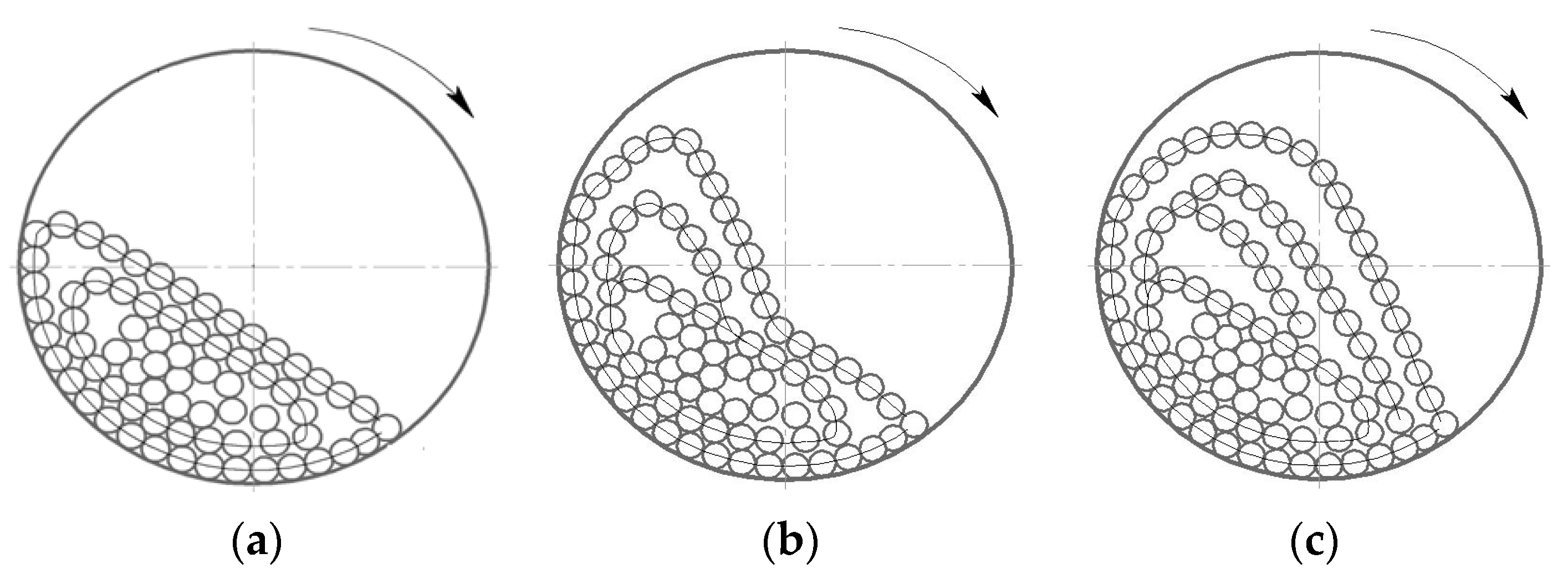
- Degree of Grinding: High ball speeds result in more intense grinding of materials, which can be useful for obtaining a finer structure. Low rotational speeds may be preferred for coarser grinding [5].
- Grinding Time: Increasing the rotational speed of the ball mill can reduce the time required to achieve the desired degree of comminution. However, a speed that is too high can lead to both over-grinding and under-grinding on the one hand, resulting in unnecessary energy loss on the other [6].
- Energy consumption: Increasing the rotational speed of the ball mill requires more energy. It is therefore important to find the optimum speed that provides the desired grinding quality with minimum energy consumption [7].
- Final product: Changing the rotational speed can influence the properties of the final product, such as the particle size, size distribution and material structure [8].
2. Analysis of the Grinding Process and Wear
3. Methods
3.1. Laboratory Study
3.2. Numerical Experiment
3.3. Numerical Methods
3.3.1. Wear Model
3.3.2. Energy of Particle Breakage
3.3.3. Model Predictive Control
4. Results
4.1. Experimental Results
4.2. Numerical Results
4.2.1. Energy Spectra
4.2.2. Lining Wear Modeling
4.3. Model of Predictive Control
5. Discussion
6. Conclusions
- The choice of liner type and material has a significant influence on the grinding process in SAG mills. In the process of lining wear, the character of the medium movement will change, and, as a consequence, the material grinding rate and the overall energy efficiency of the process will also change. In addition, the process data obtained will allow for rational planning and longer maintenance intervals in the future.
- The mill speed control during the grinding process by means of a frequency drive will be the most rational solution. In the case of the developed control strategy, changing the speed increases the grinding performance, as the rise and subsequent fall of ore increases, provided that the mill does not run to the critical speed.
- The model proposed in this manuscript for determining the optimum speed can be used both as an advisor to the process operator and as part of the control system. It should be noted that the software application is not universal and should be customized for each mill, taking into account their properties and parameters.
7. Patents
Author Contributions
Funding
Institutional Review Board Statement
Informed Consent Statement
Data Availability Statement
Conflicts of Interest
References
- Pelevin, A.E. Iron ore beneficiation technologies in Russia and ways to improve their efficiency. J. Min. Inst. 2022, 256, 579–592. [Google Scholar] [CrossRef]
- Litvinenko, V.S.; Petrov, E.I.; Vasilevskaya, D.V.; Yakovenko, A.V.; Naumov, I.A.; Ratnikov, M.A. Assessment of the role of the state in the management of mineral resources. J. Min. Inst. 2023, 259, 95–111. [Google Scholar] [CrossRef]
- Aleksandrova, T.; Nikolaeva, N.; Afanasova, A.; Romashev, A.; Kuznetsov, V. Justification for Criteria for Evaluating Activation and Destruction Processes of Complex Ores. Minerals 2023, 13, 684. [Google Scholar] [CrossRef]
- Morrell, S. Helping to reduce mining industry carbon emissions: A step-by-step guide to sizing and selection of energy efficient high pressure grinding rolls circuits. Miner. Eng. 2022, 179, 107431. [Google Scholar] [CrossRef]
- Bian, X.; Wang, G.; Wang, H.; Wang, S.; Lv, W. Effect of lifters and mill speed on particle behaviour, torque, and power consumption of a tumbling ball mill: Experimental study and DEM simulation. Miner. Eng. 2017, 105, 22–35. [Google Scholar] [CrossRef]
- Bardinas, J.P.; Aldrich, C.; Napier, L.F.A. Predicting the Operating States of Grinding Circuits by Use of Recurrence Texture Analysis of Time Series Data. Processes 2018, 6, 17. [Google Scholar] [CrossRef]
- Avalos, S.; Kracht, W.; Ortiz, J.M. Machine Learning and Deep Learning Methods in Mining Operations: A Data-Driven SAG Mill Energy Consumption Prediction Application. Min. Metall. Explor. 2020, 37, 1197–1212. [Google Scholar] [CrossRef]
- Steyn, C.W.; Sandrock, C. Benefits of optimisation and model predictive control on a fully autogenous mill with variable speed. Miner. Eng. 2013, 53, 113–123. [Google Scholar] [CrossRef]
- Cleary, P.W.; Morrison, R.D.; Delaney, G.W. Incremental damage and particle size reduction in a pilot SAG mill: DEM breakage method extension and validation. Miner. Eng. 2018, 128, 56–68. [Google Scholar] [CrossRef]
- Hasankhoei, A.R.; Maleki-Moghaddam, M.; Haji-Zadeh, A.; Barzgar, M.E.; Banisi, S. On dry SAG mills end liners: Physical modeling, DEM-based characterization and industrial outcomes of a new design. Miner. Eng. 2019, 141, 105835. [Google Scholar] [CrossRef]
- Imaichi, K.; Nordell, L.K.; Porter, B.; Potapov, A. Development and performance variation of energy saving type comminution machine using general purpose DEM simulation soft “rOCKY. ” J. Soc. Powder Technol. Japan 2017, 54, 666–672. [Google Scholar] [CrossRef]
- Cleary, P.W.; Owen, P. Effect of operating condition changes on the collisional environment in a SAG mill. Miner. Eng. 2019, 132, 297–315. [Google Scholar] [CrossRef]
- Faria, P.M.C.; Rajamani, R.K.; Tavares, L.M. Optimization of Solids Concentration in Iron Ore Ball Milling through Modeling and Simulation. Minerals 2019, 9, 366. [Google Scholar] [CrossRef]
- Cundall, P.A.; Strack, O.D.L. A discrete numerical model for granular assemblies. Geotechnique 1979, 29, 47–65. [Google Scholar] [CrossRef]
- Owen, P.; Cleary, P.W. The relationship between charge shape characteristics and fill level and lifter height for a SAG mill. Miner. Eng. 2015, 83, 19–32. [Google Scholar] [CrossRef]
- Yin, Z.; Peng, Y.; Li, T.; Wu, G. DEM Investigation of Mill Speed and Lifter Face Angle on Charge Behavior in Ball Mills. IOP Conf. Ser. Mater. Sci. Eng. 2018, 394, 032084. [Google Scholar] [CrossRef]
- Yin, Z.; Peng, Y.; Li, T.; Zhu, Z.; Yu, Z.; Wu, G. Effect of the operating parameter and grinding media on the wear properties of lifter in ball mills. Proc. Inst. Mech. Eng. Part J J. Eng. Tribol. 2019, 234, 1061–1074. [Google Scholar] [CrossRef]
- Bolobov, V.I.; Latipov, I.U.; Zhukov, V.S.; Popov, G.G. Using the Magnetic Anisotropy Method to Determine Hydrogenated Sections of a Steel Pipeline. Energies 2023, 16, 5585. [Google Scholar] [CrossRef]
- Hu, Q.; Ji, D.; Shen, M.; Zhuang, H.; Yao, H.; Zhao, H.; Guo, H.; Zhang, Y. Three-Body Abrasive Wear Behavior of WC-10Cr3C2-12Ni Coating for Ball Mill Liner Application. Materials 2022, 15, 4569. [Google Scholar] [CrossRef]
- Wu, W.; Che, H.; Hao, Q. Research on Non-Uniform Wear of Liner in SAG Mill. Processes 2020, 8, 1543. [Google Scholar] [CrossRef]
- Liu, Z.; Wang, G.; Guan, W.; Guo, J.; Sun, G.; Chen, Z. Research on performance of a laboratory-scale SAG mill based on DEM-EMBD. Powder Technol. 2022, 406, 117581. [Google Scholar] [CrossRef]
- Cleary, P.W.; Hilton, J.E.; Sinnott, M.D. Modelling of industrial particle and multiphase flows. Powder Technol. 2017, 314, 232–252. [Google Scholar] [CrossRef]
- Cleary, P.W.; Owen, P. Development of models relating charge shape and power draw to SAG mill operating parameters and their use in devising mill operating strategies to account for liner wear. Miner. Eng. 2018, 117, 42–62. [Google Scholar] [CrossRef]
- Gizatullin, R.; Dvoynikov, M.; Romanova, N.; Nikitin, V. Drilling in Gas Hydrates: Managing Gas Appearance Risks. Energies 2023, 16, 2387. [Google Scholar] [CrossRef]
- Kozhubaev, Y.; Belyaev, V.; Murashov, Y.; Prokofev, O. Controlling of Unmanned Underwater Vehicles Using the Dynamic Planning of Symmetric Trajectory Based on Machine Learning for Marine Resources Exploration. Symmetry 2023, 15, 1783. [Google Scholar] [CrossRef]
- Rogachev, M.K.; Aleksandrov, A.N. Justification of a comprehensive technology for preventing the formation of asphalt-resin-paraffin deposits during the production of highly paraffinic oil by electric submersible pumps from multiformation deposits. J. Min. Inst. 2021, 250, 596–605. [Google Scholar] [CrossRef]
- Martynov, S.A.; Pervukhin, D.A. Algorithm for calculating of the carbon-graphite electrode consumption in an ore-thermal furnace and its position at different stages of smelting. Chernye Met. 2023, 2023, 8–15. [Google Scholar] [CrossRef]
- Greenwood, J.A.; Tripp, J.H. The Contact of Two Nominally Flat Rough Surfaces. Proc. Inst. Mech. Eng. 1970, 185, 625–633. [Google Scholar] [CrossRef]
- Fleischer, G. Energetische Methode der Bestimmung des Verschleisses. Schmierungstechnik 1973, 4, 269–274. [Google Scholar]
- Kragelsky, I.V.; Dobychin, M.N.; Kombalov, V.S. Friction and Wear, 1st ed.; Springer: Berlin/Heidelberg, Germany, 1982. [Google Scholar]
- Archard, J.F. Contact and rubbing of flat surfaces. J. Appl. Phys. 1953, 24, 981–988. [Google Scholar] [CrossRef]
- Varenberg, M. Adjusting for Running-in: Extension of the Archard Wear Equation. Tribol. Lett. 2022, 70, 1–8. [Google Scholar] [CrossRef]
- Morrison, R.D.; Cleary, P.W. Using DEM to model ore breakage within a pilot scale SAG mill. Miner. Eng. 2004, 17, 1117–1124. [Google Scholar] [CrossRef]
- Bolobov, V.I.; Chupin, S.A.; Le-Thanh, B. Modeling impact fracture of rock by hydraulic hammer pick with regard to its bluntness. Eurasian Min. 2022, 37, 72–75. [Google Scholar] [CrossRef]
- Boikov, A.; Savelev, R.; Payor, V.; Potapov, A. Universal Approach for DEM Parameters Calibration of Bulk Materials. Symmetry 2021, 13, 1088. [Google Scholar] [CrossRef]
- Weerasekara, N.S.; Liu, L.X.; Powell, M.S. Estimating energy in grinding using DEM modelling. Miner. Eng. 2016, 85, 23–33. [Google Scholar] [CrossRef]
- Lvov, V.; Chitalov, L. Semi-autogenous wet grinding modeling with cfd-dem. Minerals 2021, 11, 485. [Google Scholar] [CrossRef]
- Zhukovskiy, Y.L.; Korolev, N.A.; Malkova, Y.M. Monitoring of grinding condition in drum mills based on resulting shaft torque. J. Min. Inst. 2022, 256, 686–700. [Google Scholar] [CrossRef]
- Cleary, P.W.; Morrison, R.D.; Sinnott, M.D. Prediction of slurry grinding due to media and coarse rock interactions in a 3D pilot SAG mill using a coupled DEM + SPH model. Miner. Eng. 2020, 159, 106614. [Google Scholar] [CrossRef]
- Vasilyeva, N.; Golyshevskaia, U.; Sniatkova, A. Modeling and Improving the Efficiency of Crushing Equipment. Symmetry 2023, 15, 1343. [Google Scholar] [CrossRef]
- Goldobina, L.A.; Demenkov, P.A.; Trushko, O.V. Ensuring the safety of construction works during the erection of buildings and structures. J. Min. Inst. 2019, 239, 583–595. [Google Scholar] [CrossRef]
- Bemporad, A. Model Predictive Control design: New trends and tools. In Proceedings of the 45th IEEE Conference on Decision and Control, San Diego, CA, USA, 13–15 December 2006; pp. 6678–6683. [Google Scholar] [CrossRef]
- Zanoli, S.M.; Pepe, C.; Astolfi, G. Advanced Process Control for Clinker Rotary Kiln and Grate Cooler. Sensors 2023, 23, 2805. [Google Scholar] [CrossRef]
- César, G.Q.; Daniel, S.H. Multivariable Model Predictive Control of a Simulated SAG plant. IFAC Proc. Vol. 2009, 42, 37–42. [Google Scholar] [CrossRef]
- BrainWave SAG Mill. Available online: https://www.andritz.com/products-en/automation/advanced-process-control/brainwave-sag-mill (accessed on 23 November 2023).
- Chen, S.; Zhang, T.; Zou, Y.; Xiao, M. Model predictive control of robotic grinding based on deep belief network. Complexity 2019, 2019, 1891365. [Google Scholar] [CrossRef]
- Delaney, G.W.; Cleary, P.W.; Morrison, R.D.; Cummins, S.; Loveday, B. Predicting breakage and the evolution of rock size and shape distributions in Ag and SAG mills using DEM. Miner. Eng. 2013, 50–51, 132–139. [Google Scholar] [CrossRef]
- Saldaña, M.; Gálvez, E.; Navarra, A.; Toro, N.; Cisternas, L.A. Optimization of the SAG Grinding Process Using Statistical Analysis and Machine Learning: A Case Study of the Chilean Copper Mining Industry. Materials 2023, 16, 3220. [Google Scholar] [CrossRef] [PubMed]
- Bolobov, V.I.; Chupin, S.A.; Akhmerov, E.V.; Plaschinskiy, V.A. Comparative Wear Resistance of Existing and Prospective Materials of Fast-Wearing Elements of Mining Equipment. Mater. Sci. Forum 2021, 1040, 117–123. [Google Scholar] [CrossRef]
- Shishlyannikov, D.I.; Lavrenko, S.A.; Zverev, V.Y.; Muravskiy, A.K.; Mikryukov, A.Y. Hydroabrasive wear of work stages of electric-centrifugal well pumps for fluids with high content of mechanical impurities. Min. Informational Anal. Bull. 2023, 2023, 5–20. [Google Scholar]
- Serzhan, S.L.; Skrebnev, V.I.; Malevanny, D.V. Study of the effects of steel and polymer pipe roughness on the pressure loss in tailings slurry hydrotransport. Obogashchenie Rud 2023, 4, 41–49. [Google Scholar] [CrossRef]
- Beloglazov, I.I.; Sabinin, D.S.; Nikolaev, M.Y.U. Modeling the disintegration process for ball mills using dem. Min. Informational Anal. Bull. 2022, 268–282. [Google Scholar] [CrossRef]
- Boemer, D.; Carretta, Y.; Laugier, M.; Legrand, N.; Papeleux, L.; Boman, R.; Ponthot, J.P. An advanced model of lubricated cold rolling with its comprehensive pilot mill validation. J. Mater. Process. Technol. 2021, 296, 117175. [Google Scholar] [CrossRef]
- Cleary, P.W.; Delaney, G.W.; Sinnott, M.D.; Morrison, R.D. Inclusion of incremental damage breakage of particles and slurry rheology into a particle scale multiphase model of a SAG mill. Miner. Eng. 2018, 128, 92–105. [Google Scholar] [CrossRef]
- Fedorova, E.R.; Vinogradova, A.A. Generalized mathematical model of red muds’ thickener of alumina production. IOP Conf. Ser. Mater. Sci. Eng. 2018, 327, 022031. [Google Scholar] [CrossRef]
- Fedorova, E.R.; Pupysheva, E.A.; Morgunov, V.V. Settling parameters determined during thickening and washing of red muds. Tsvetnye Met. 2023, 2023, 77–84. [Google Scholar] [CrossRef]
- Nikolaichuk, L.; Ignatiev, K.; Filatova, I.; Shabalovac, A. Diversification of Portfolio of International Oil and Gas Assets using Cluster Analysis. Int. J. Eng. 2023, 36, 1783–1792. [Google Scholar] [CrossRef]
- King, R.P. Comminution operations. In Modeling and Simulation of Mineral Processing Systems; Elsevier: Amsterdam, The Netherlands, 2001; pp. 127–212. [Google Scholar] [CrossRef]
- Srivastava, V.; Akdogan, G.; Ghosh, T.; Ganguli, R. Dynamic modeling and simulation of a SAG mill for mill charge characterization. Miner. Metall. Process. 2018, 35, 61–68. [Google Scholar] [CrossRef]
- Kulchitskiy, A. Optical Inspection Systems for Axisymmetric Parts with Spatial 2D Resolution. Symmetry 2021, 13, 1218. [Google Scholar] [CrossRef]
- Global Mining Guidelines Group. The Morrell Method to Determine the Efficiency of Industrial Grinding Circuits. Available online: https://gmggroup.org/guidelines-and-publications/morrell-method-to-determine-the-efficiency-of-industrial-grinding-circuits/ (accessed on 23 December 2023).
- Nguyen, V.T.; Pham, T.V.; Rogachev, M.K.; Korobov, G.Y.; Parfenov, D.V.; Zhurkevich, A.O.O.; Islamov, S.R. A comprehensive method for determining the dewaxing interval period in gas lift wells. J. Pet. Explor. Prod. Technol. 2023, 13, 1163–1179. [Google Scholar] [CrossRef]
- Real-Time Estimation of SAG Mill Charge Characteristics for Process Optimization. Available online: https://www.researchgate.net/publication/374368429_Real-Time_Estimation_of_SAG_Mill_Charge_Characteristics_for_Process_Optimization (accessed on 23 December 2023).


| Property | Material | Balls | Lining |
|---|---|---|---|
| Density, kg/m3 | 3.2 × 10³ | 7.7 × 10³ | 7.7 × 10³ |
| Young’s modulus, N/m | 1 × 10⁸ | 2 × 10¹¹ | 2 × 10¹¹ |
| Rolling resistance | 0.15 | 0.001 | 0.05 |
| Poisson’s ratio | 0.25 | 0.3 | 0.3 |
| Fraction size, m | 0.18–50% | 0.1 | - |
| 0.06–30% | |||
| 0.03–20% | |||
| Ball loading and material, kg | 4 × 10³ | 15.8 × 10³ | - |
| Interaction Parameter | Material–Material | Material–Balls | Material–Lining | Balls–Lining | Balls–Balls |
|---|---|---|---|---|---|
| Friction coefficient | 0.87 | 0.5 | 0.3 | 0.15 | 0.15 |
| Restitution coefficient | 0.5 | 0.5 | 0.3 | 0.15 | 0.5 |
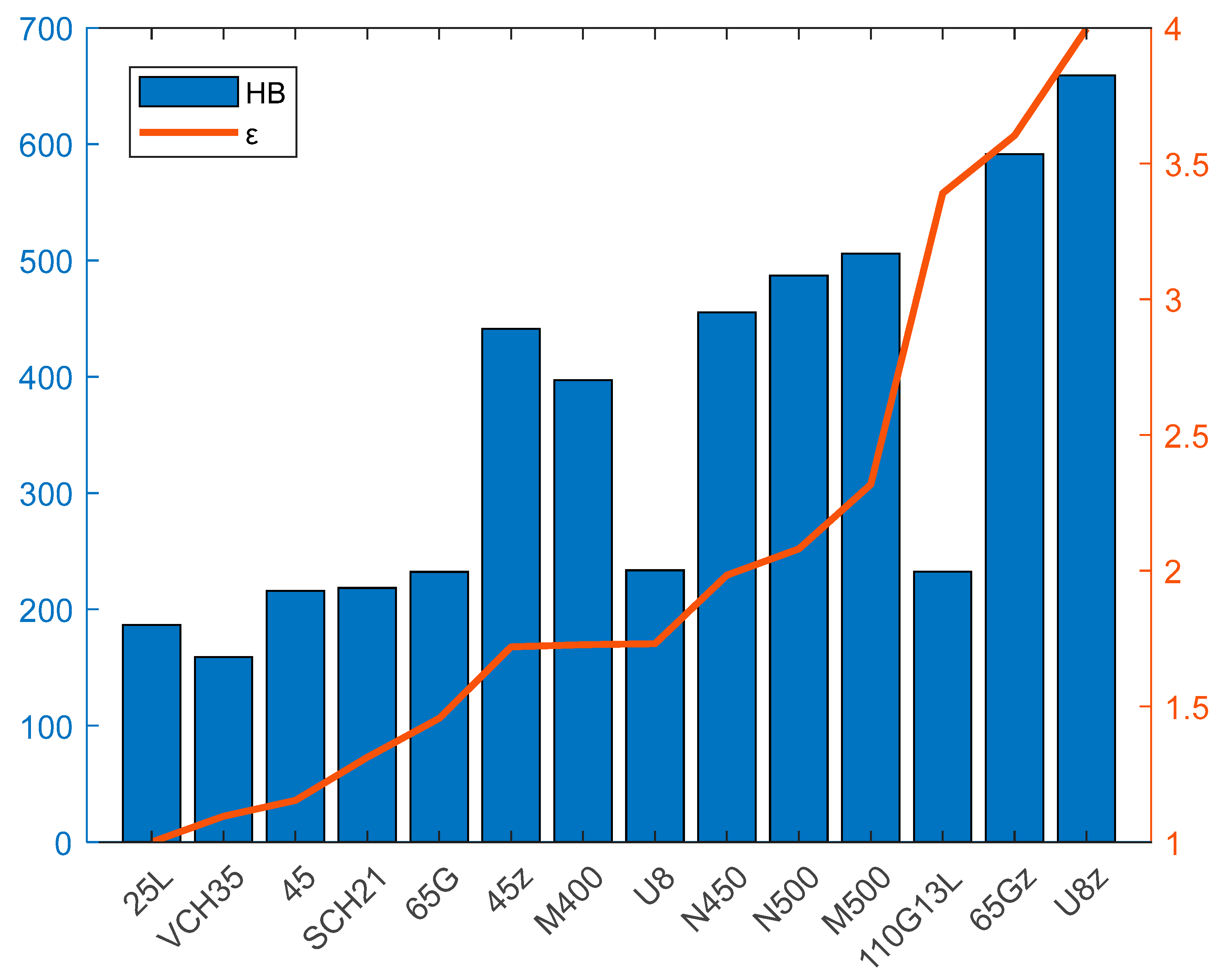
| Material | Vi, g/min | Ii, min/g | ε | HB |
|---|---|---|---|---|
| 25L | 0.53 | 1.90 | 1.0 | 186.8 |
| BCH35 | 0.48 | 2.08 | 1.1 | 159.1 |
| 45 | 0.46 | 2.19 | 1.2 | 216.1 |
| SCH21 | 0.40 | 2.49 | 1.3 | 218.6 |
| 65G | 0.36 | 2.76 | 1.5 | 232.4 |
| 45z | 0.31 | 3.26 | 1.7 | 441.3 |
| M400 | 0.31 | 3.27 | 1.7 | 397.0 |
| U8 | 0.30 | 3.28 | 1.7 | 233.8 |
| N450 | 0.27 | 3.76 | 2.0 | 455.4 |
| N500 | 0.25 | 3.94 | 2.1 | 486.9 |
| M500 | 0.23 | 4.39 | 2.3 | 506.0 |
| 110G13L | 0.16 | 6.43 | 3.4 | 232.5 |
| 65Gz | 0.15 | 6.83 | 3.6 | 591.5 |
| U8z | 0.13 | 7.58 | 4.0 | 659.0 |
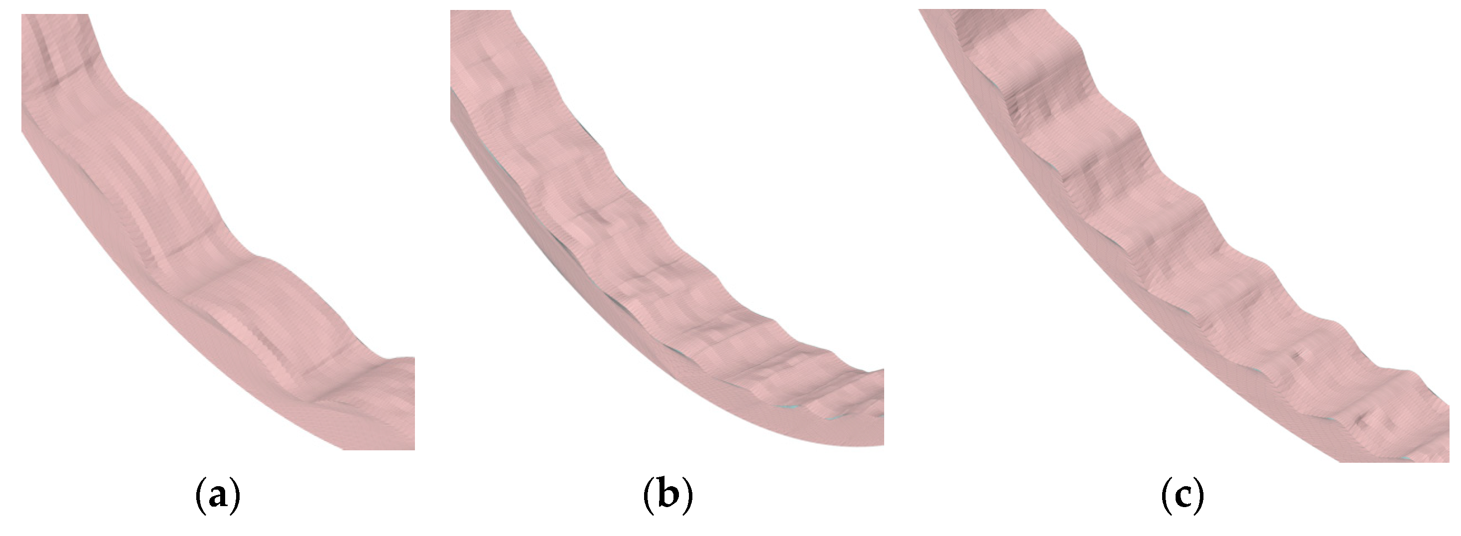
| Type of Lining | Linear Size of Lining Protrusion L, m | Linear Wear of Lining Profile ∆l, m | Total Volume of Lining V, m3 | Volume after Modeling V, m3 | Loss of Lining Volume ΔV, m3 | Percentage of Worn Surface L, % |
|---|---|---|---|---|---|---|
| K = 1 × 10⁻⁵ | ||||||
| type 1 | 0.076 | 0.03 | 0.085 | 0.032 | 0.053 | 39 |
| type 2 | 0.076 | 0.045 | 0.087 | 0.014 | 0.073 | 59 |
| type 3 | 0.076 | 0.05 | 0.092 | 0.010 | 0.082 | 65 |
| Steel | HB | K | Et, MJ | Vi, g/min | Vm, g/min |
|---|---|---|---|---|---|
| 45L | 200 | 1 × 10⁻⁶ | 174.00 | 0.46 | 0.84 |
| 110G13L | 235 | 2.5 × 10⁻⁶ | 204.45 | 0.16 | 0.75 |
| H450 | 450 | 7 × 10⁻⁶ | 391.50 | 0.27 | 0.44 |
Disclaimer/Publisher’s Note: The statements, opinions and data contained in all publications are solely those of the individual author(s) and contributor(s) and not of MDPI and/or the editor(s). MDPI and/or the editor(s) disclaim responsibility for any injury to people or property resulting from any ideas, methods, instructions or products referred to in the content. |
© 2024 by the authors. Licensee MDPI, Basel, Switzerland. This article is an open access article distributed under the terms and conditions of the Creative Commons Attribution (CC BY) license (https://creativecommons.org/licenses/by/4.0/).
Share and Cite
Beloglazov, I.; Plaschinsky, V. Development MPC for the Grinding Process in SAG Mills Using DEM Investigations on Liner Wear. Materials 2024, 17, 795. https://doi.org/10.3390/ma17040795
Beloglazov I, Plaschinsky V. Development MPC for the Grinding Process in SAG Mills Using DEM Investigations on Liner Wear. Materials. 2024; 17(4):795. https://doi.org/10.3390/ma17040795
Chicago/Turabian StyleBeloglazov, Ilia, and Vyacheslav Plaschinsky. 2024. "Development MPC for the Grinding Process in SAG Mills Using DEM Investigations on Liner Wear" Materials 17, no. 4: 795. https://doi.org/10.3390/ma17040795