

Accelerating Elastic Property Prediction in Fe-C Alloys through Coupling of Molecular Dynamics and Machine Learning
 ,
,
Abstract
:1. Introduction
2. Data and Methods
2.1. Potential Development
2.2. Data Collection/Calculation
2.3. Input Parameters
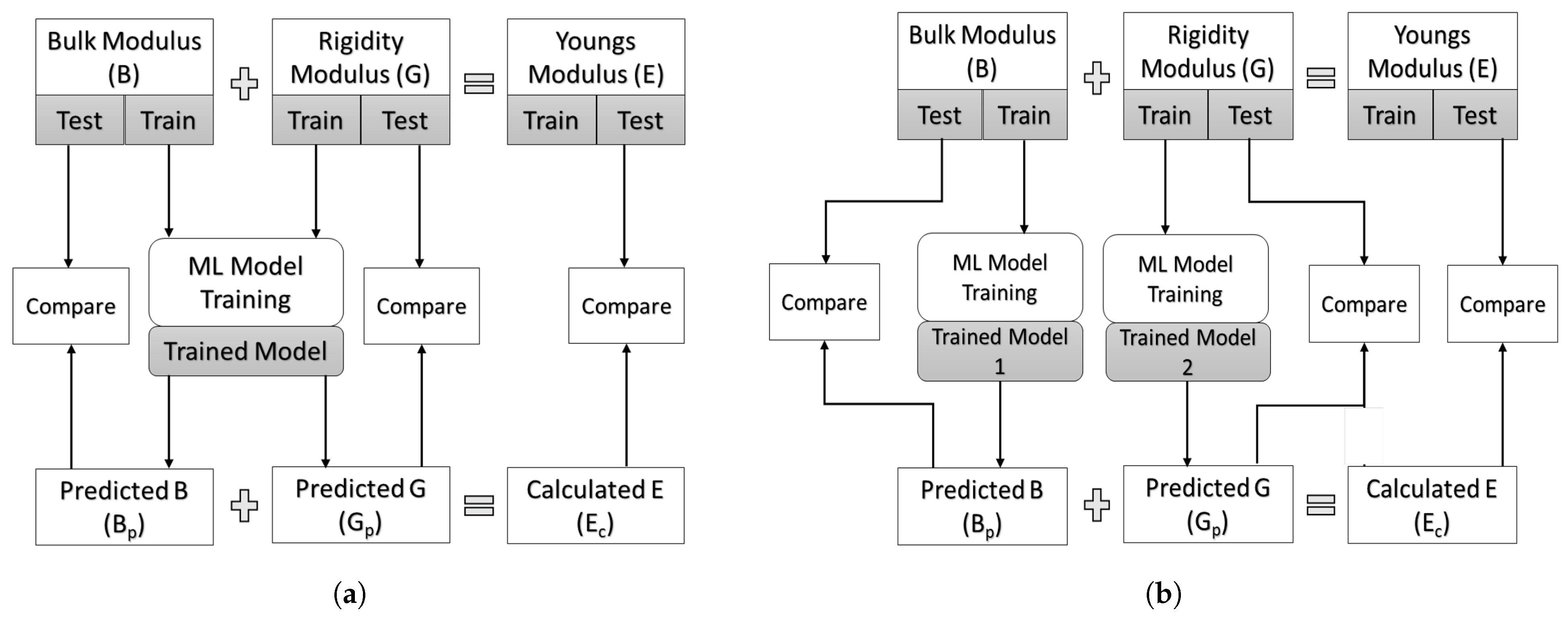
2.4. ML Algorithms
2.4.1. Random Forest (RF)
2.4.2. Extreme Gradient Boosting (XGBoost)
2.4.3. Support Vector Machine (SVM)
2.4.4. K-Nearest Neighbor (KNN)
2.4.5. MultiLayer Perceptron (MLP)
2.4.6. Gaussian Process Regression (GPR)
2.4.7. Super Learner (SL)
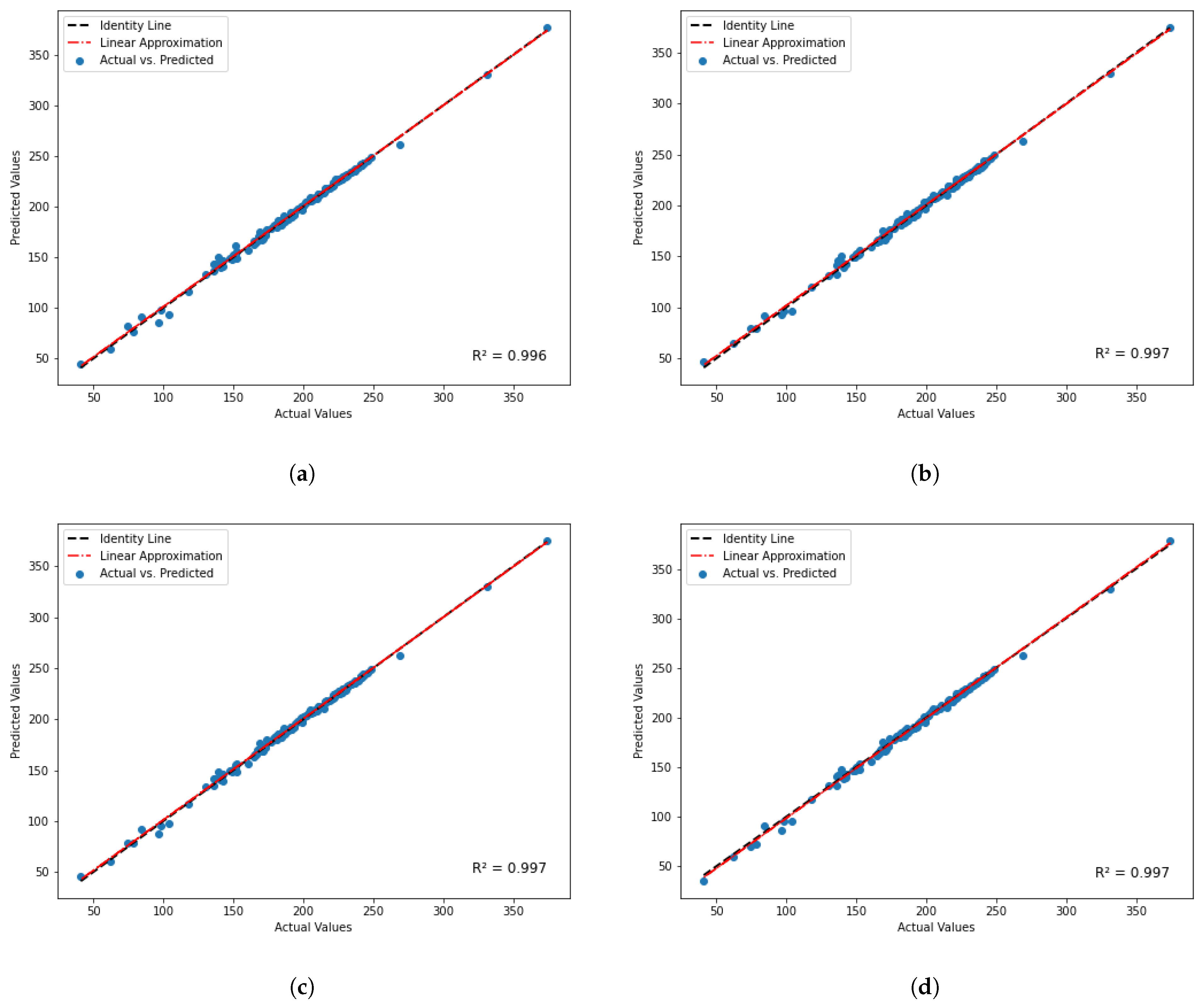
3. Results and Discussion
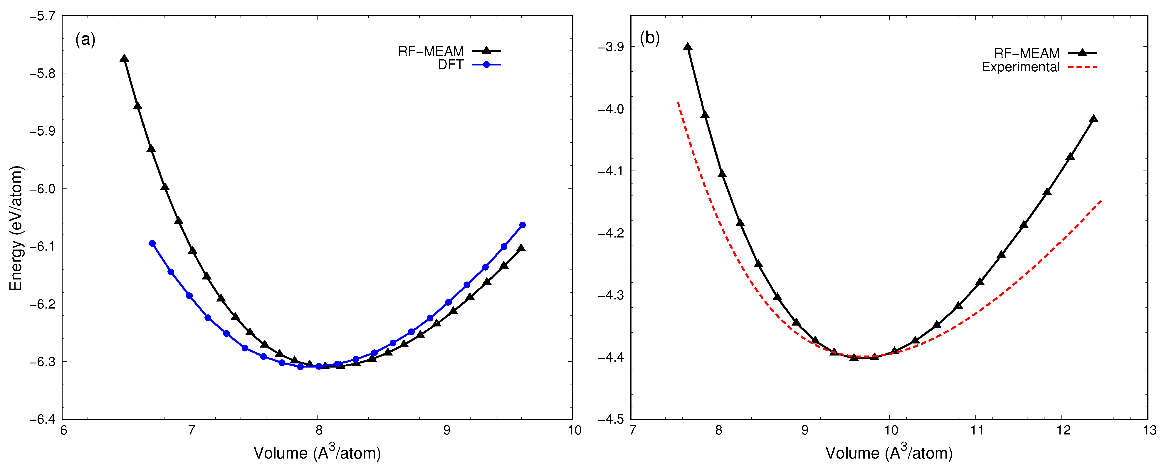
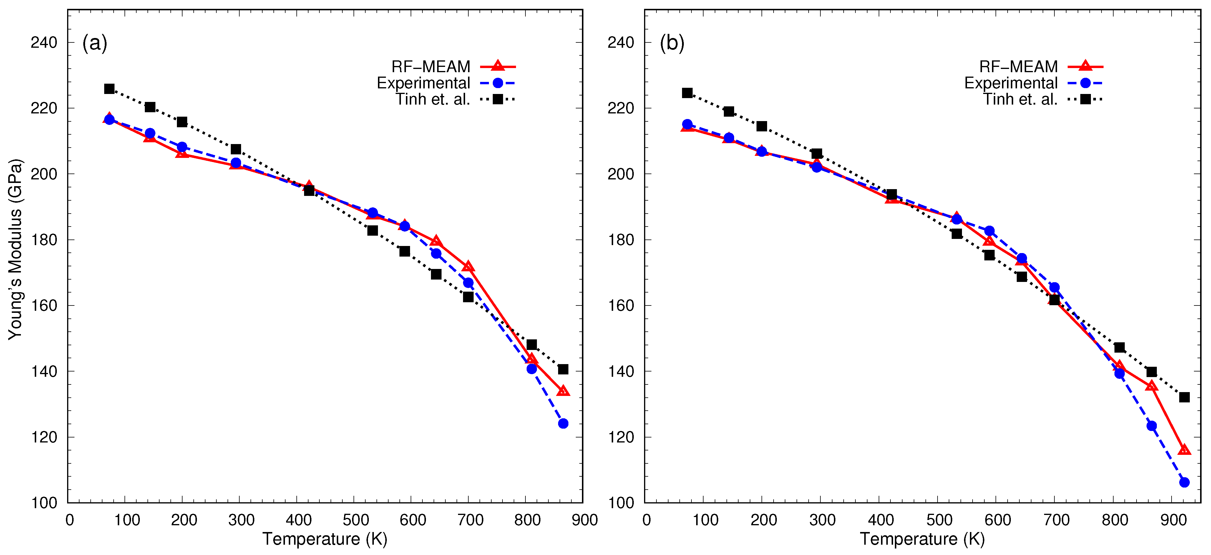
3.1. Potential Verification
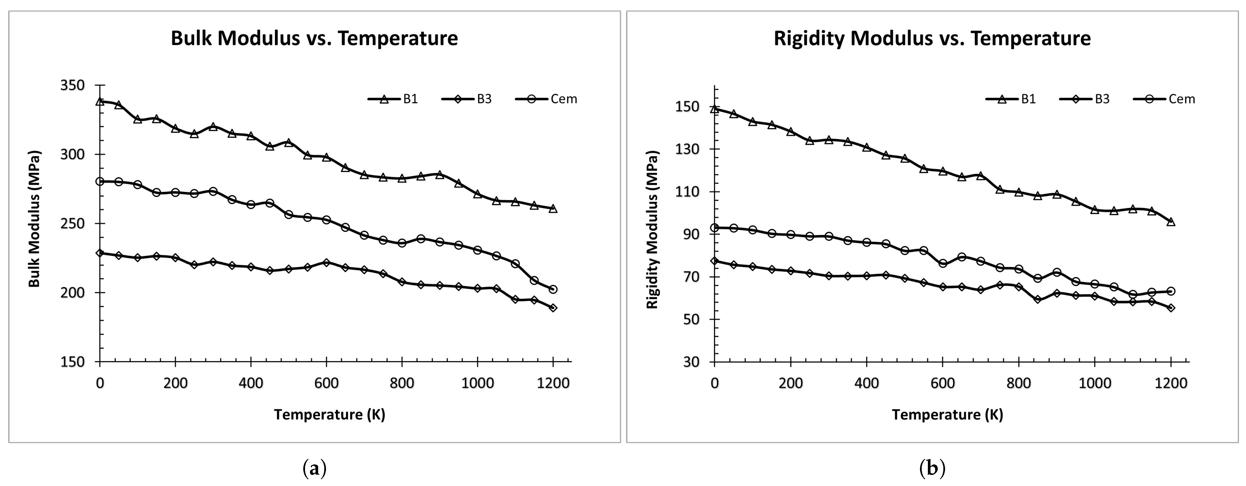
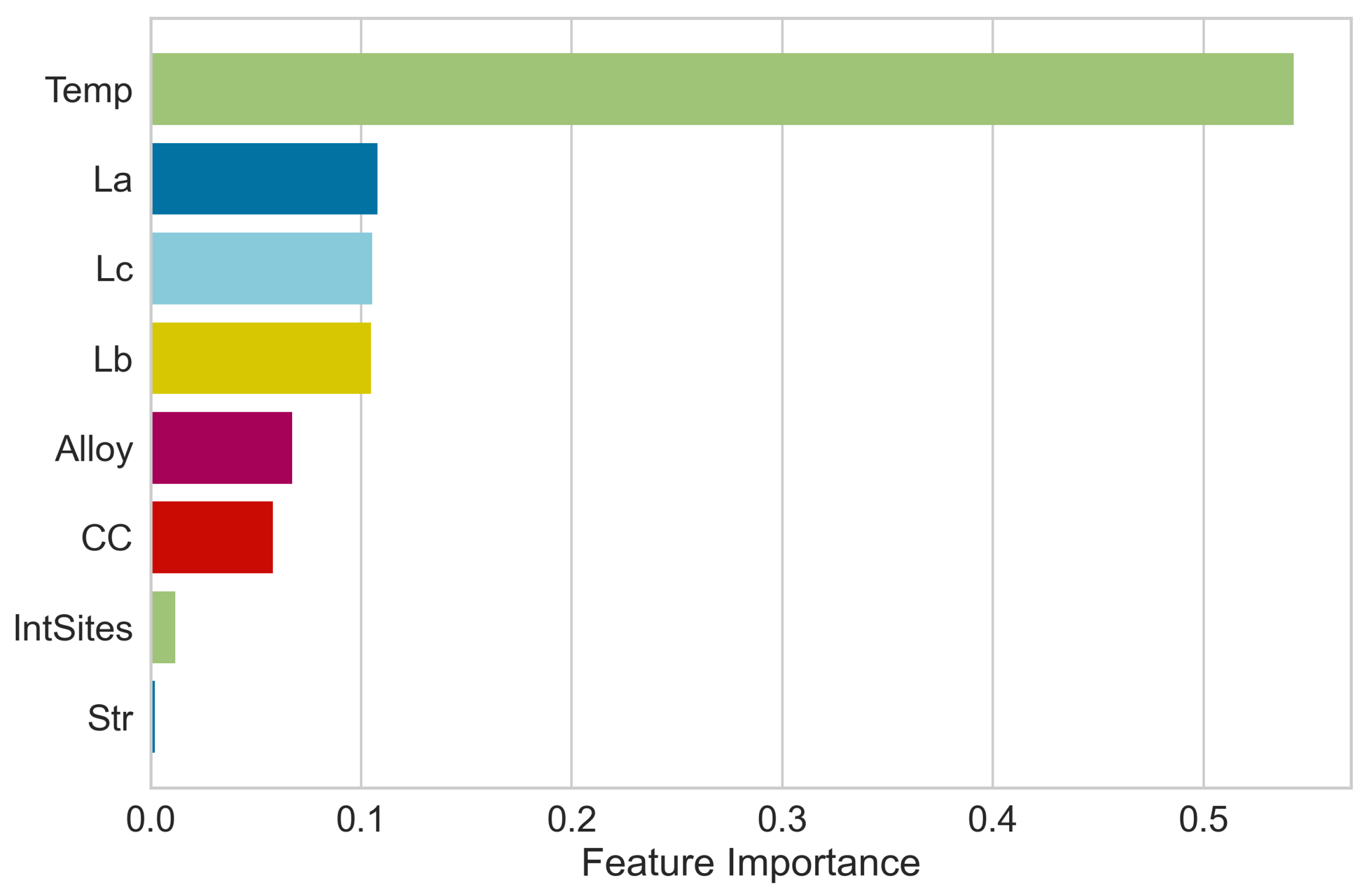
3.2. Data Analysis and Feature Selection
3.3. Feature Elimination and Hyperparameter Tuning
4. Conclusions
Author Contributions
Funding
Institutional Review Board Statement
Informed Consent Statement
Data Availability Statement
Acknowledgments
Conflicts of Interest
References
- Chen, L.; Chen, L.; Kalinin, S.; Klimeck, G.; Kumar, S.; Neugebauer, J.; Terasaki, I. Design and discovery of materials guided by theory and computation. NPJ Comput. Mater. 2015, 1, 1–2. [Google Scholar] [CrossRef]
- Singh, V.; Patra, S.; Murugan, N.; Toncu, D.; Tiwari, A. Recent trends in computational tools and data-driven modeling for advanced materials. Mater. Adv. 2022, 3, 4069–4087. [Google Scholar] [CrossRef]
- Vandenhaute, S.; Rogge, S.; Van Speybroeck, V. Large-scale molecular dynamics simulations reveal new insights into the phase transition mechanisms in MIL-53 (Al). Front. Chem. 2021, 9, 718920. [Google Scholar] [CrossRef]
- Allen, M.; Tildesley, D. Computer Simulation of Liquids; Oxford University Press: Oxford, UK, 2017. [Google Scholar]
- Tuckerman, M. Statistical Mechanics: Theory and Molecular Simulation; Oxford University Press: Oxford, UK, 2023. [Google Scholar]
- Fujisaki, H.; Moritsugu, K.; Matsunaga, Y.; Morishita, T.; Maragliano, L. Extended phase-space methods for enhanced sampling in molecular simulations: A review. Front. Bioeng. Biotechnol. 2015, 3, 125. [Google Scholar] [CrossRef] [PubMed]
- Bernardi, R.; Melo, M.; Schulten, K. Enhanced sampling techniques in molecular dynamics simulations of biological systems. Biochim. Biophys. Acta 2015, 1850, 872. [Google Scholar] [CrossRef] [PubMed]
- Mueller, T.; Kusne, A.; Ramprasad, R. Machine learning in materials science: Recent progress and emerging applications. Rev. Comput. Chem. 2016, 29, 186–273. [Google Scholar]
- Nosengo, N. Can artificial intelligence create the next wonder material? Nature 2016, 533, 22–25. [Google Scholar] [CrossRef] [PubMed]
- Butler, K.; Davies, D.; Cartwright, H.; Isayev, O.; Walsh, A. Machine learning for molecular and materials science. Nature 2018, 559, 547–555. [Google Scholar] [CrossRef] [PubMed]
- Schmidt, J.; Marques, M.; Botti, S.; Marques, M. Recent advances and applications of machine learning in solid-state materials science. Npj Comput. Mater. 2019, 5, 83. [Google Scholar] [CrossRef]
- Risal, S.; Zhu, W.; Guillen, P.; Sun, L. Improving phase prediction accuracy for high entropy alloys with Machine learning. Comput. Mater. Sci. 2021, 192, 110389. Available online: https://www.sciencedirect.com/science/article/pii/S0927025621001142 (accessed on 23 October 2023). [CrossRef]
- Hu, M.; Tan, Q.; Knibbe, R.; Wang, S.; Li, X.; Wu, T.; Jarin, S.; Zhang, M. Prediction of mechanical properties of wrought aluminium alloys using feature engineering assisted machine learning approach. Metall. Mater. Trans. A 2021, 52, 2873–2884. [Google Scholar] [CrossRef]
- Deng, Z.; Yin, H.; Jiang, X.; Zhang, C.; Zhang, G.; Xu, B.; Yang, G.; Zhang, T.; Wu, M.; Qu, X. Machine-learning-assisted prediction of the mechanical properties of Cu-Al alloy. Int. J. Miner. Metall. Mater. 2020, 27, 362–373. [Google Scholar] [CrossRef]
- Devi, M.; Prakash, C.; Chinnannavar, R.; Joshi, V.; Palada, R.; Dixit, R. An informatic approach to predict the mechanical properties of aluminum alloys using machine learning techniques. In Proceedings of the 2020 International Conference on Smart Electronics and Communication (ICOSEC), Trichy, India, 10–12 September 2020; pp. 536–541. [Google Scholar]
- Xu, X.; Wang, L.; Zhu, G.; Zeng, X. Predicting tensile properties of AZ31 magnesium alloys by machine learning. JOM 2020, 72, 3935–3942. [Google Scholar] [CrossRef]
- Choyi, Y. Computational Alloy Design and Discovery Using Machine Learning. 2020. Available online: https://www.semanticscholar.org/paper/Computational-Alloy-Design-and-Discovery-Using-Choyi/c2648b0cc575cf288e778857f6dbcad357b46e9a (accessed on 21 December 2023).
- Ling, J.; Antono, E.; Bajaj, S.; Paradiso, S.; Hutchinson, M.; Meredig, B.; Gibbons, B. Machine learning for alloy composition and process optimization. Turbo Expo Power Land Sea Air 2018, 51128, V006T24A005. [Google Scholar]
- Lu, J.; Chen, Y.; Xu, M. Prediction of mechanical properties of Mg-rare earth alloys by machine learning. Mater. Res. Express 2022, 9, 106519. [Google Scholar] [CrossRef]
- Tan, R.; Li, Z.; Zhao, S.; Birbilis, N. A primitive machine learning tool for the mechanical property prediction of multiple principal element alloys. arXiv 2023, arXiv:2308.07649. [Google Scholar]
- Zhang, Q.; Mahfouf, M. Fuzzy predictive modelling using hierarchical clustering and multi-objective optimisation for mechanical properties of alloy steels. IFAC Proc. Vol. 2007, 40, 427–432. [Google Scholar] [CrossRef]
- Lee, J.; Park, C.; Do Lee, B.; Park, J.; Goo, N.; Sohn, K. A machine-learning-based alloy design platform that enables both forward and inverse predictions for thermo-mechanically controlled processed (TMCP) steel alloys. Sci. Rep. 2021, 11, 11012. [Google Scholar] [CrossRef] [PubMed]
- Shen, C.; Wang, C.; Wei, X.; Li, Y.; Zwaag, S.; Xu, W. Physical metallurgy-guided machine learning and artificial intelligent design of ultrahigh-strength stainless steel. Acta Mater. 2019, 179, 201–214. [Google Scholar] [CrossRef]
- Mahfouf, M. Optimal design of alloy steels using genetic algorithms. In Advances in Computational Intelligence and Learning: Methods and Applications; Springer Science+Business Media: New York, NY, USA, 2002; pp. 425–436. [Google Scholar]
- Gaffour, S.; Mahfouf, M.; Yang, Y. ‘Symbiotic’ data-driven modelling for the accurate prediction of mechanical properties of alloy steels. In Proceedings of the 2010 5th IEEE International Conference Intelligent Systems, London, UK, 7–9 July 2010; pp. 31–36. [Google Scholar]
- Dutta, T.; Dey, S.; Datta, S.; Das, D. Designing dual-phase steels with improved performance using ANN and GA in tandem. Comput. Mater. Sci. 2019, 157, 6–16. Available online: https://www.sciencedirect.com/science/article/pii/S092702561830692X (accessed on 25 September 2023). [CrossRef]
- Pattanayak, S.; Dey, S.; Chatterjee, S.; Chowdhury, S.; Datta, S. Computational intelligence based designing of microalloyed pipeline steel. Comput. Mater. Sci. 2015, 104, 60–68. [Google Scholar] [CrossRef]
- Risal, S.; Singh, N.; Duff, A.; Yao, Y.; Sun, L.; Risal, S.; Zhu, W. Development of the RF-MEAM Interatomic Potential for the Fe-C System to Study the Temperature-Dependent Elastic Properties. Materials 2023, 16, 3779. [Google Scholar] [CrossRef]
- Kresse, G.; Hafner, J. Ab initio molecular dynamics for liquid metals. Phys. Rev. B 1993, 47, 558–561. [Google Scholar] [CrossRef]
- Kresse, G.; Joubert, D. From ultrasoft pseudopotentials to the projector augmented-wave method. Phys. Rev. B 1999, 59, 1758–1775. [Google Scholar] [CrossRef]
- Perdew, J.; Ruzsinszky, A.; Csonka, G.; Vydrov, O.; Scuseria, G.; Constantin, L.; Zhou, X.; Burke, K. Restoring the Density-Gradient Expansion for Exchange in Solids and Surfaces. Phys. Rev. Lett. 2008, 100, 136406. [Google Scholar] [CrossRef]
- Timonova, M.; Thijsse, B. Optimizing the MEAM potential for silicon. Model. Simul. Mater. Sci. Eng. 2010, 19, 015003. [Google Scholar] [CrossRef]
- Duff, A. MEAMfit: A reference-free modified embedded atom method (RF-MEAM) energy and force-fitting code. Comput. Phys. Commun. 2016, 203, 354–355. [Google Scholar] [CrossRef]
- Thompson, A.; Aktulga, H.; Berger, R.; Bolintineanu, D.; Brown, W.; Crozier, P.; Veld, P.; Kohlmeyer, A.; Moore, S.; Nguyen, T.; et al. LAMMPS-a flexible simulation tool for particle-based materials modeling at the atomic, meso, and continuum scales. Comput. Phys. Commun. 2022, 271, 108171. [Google Scholar] [CrossRef]
- Breiman, L. Random forests. Mach. Learn. 2001, 45, 5–32. [Google Scholar] [CrossRef]
- Hastie, T.; Tibshirani, R.; Friedman, J.; Hastie, T.; Tibshirani, R.; Friedman, J. Random forests. In The Elements of Statistical Learning: Data Mining, Inference, and Prediction; Springer: Berlin/Heidelberg, Germany, 2009; pp. 587–604. [Google Scholar]
- Svetnik, V.; Liaw, A.; Tong, C.; Culberson, J.; Sheridan, R.; Feuston, B. Random forest: A classification and regression tool for compound classification and QSAR modeling. J. Chem. Inf. Comput. Sci. 2003, 43, 1947–1958. [Google Scholar] [CrossRef] [PubMed]
- Chen, T.; He, T.; Benesty, M.; Khotilovich, V.; Tang, Y.; Cho, H.; Chen, K.; Mitchell, R.; Cano, I.; Zhou, T.; et al. R Package Version 0.4-2; Xgboost: Extreme gradient boosting; 2015; Volumer 1, pp. 1–4. [Google Scholar]
- Chen, T.; Guestrin, C. Xgboost: A scalable tree boosting system. In Proceedings of the 22nd Acm Sigkdd International Conference on Knowledge Discovery and Data Mining, San Francisco, CA, USA, 13–17 August 2016; pp. 785–794. [Google Scholar]
- Guillen-Rondon, P.; Robinson, M.; Torres, C.; Pereya, E. Support vector machine application for multiphase flow pattern prediction. arXiv 2018, arXiv:1806.05054. [Google Scholar]
- Steinwart, I.; Christmann, A. Support Vector Machines; Springer Science & Business Media: New York, NY, USA, 2008. [Google Scholar]
- Statnikov, A. A Gentle Introduction to Support Vector Machines in Biomedicine: Theory and Methods; World Scientific: London, UK, 2011. [Google Scholar]
- Kramer, O. K-nearest neighbors. In Dimensionality Reduction with Unsupervised Nearest Neighbors; Springer: Berlin/Heidelberg, Germany, 2013; pp. 13–23. [Google Scholar]
- Peterson, L. K-nearest neighbor. Scholarpedia 2009, 4, 1883. [Google Scholar] [CrossRef]
- Kumar, T. Solution of linear and non linear regression problem by K Nearest Neighbour approach: By using three sigma rule. In Proceedings of the 2015 IEEE International Conference on Computational Intelligence & Communication Technology, Ghaziabad, India, 13–14 February 2015; pp. 197–201. [Google Scholar]
- Skryjomski, P.; Krawczyk, B.; Cano, A. Speeding up k-Nearest Neighbors classifier for large-scale multi-label learning on GPUs. Neurocomputing 2019, 354, 10–19. Available online: https://www.sciencedirect.com/science/article/pii/S0925231219304588 (accessed on 20 September 2023). [CrossRef]
- Wu, Y.; Feng, J. Development and application of artificial neural network. Wirel. Pers. Commun. 2018, 102, 1645–1656. [Google Scholar] [CrossRef]
- Popescu, M.; Balas, V.; Perescu-Popescu, L.; Mastorakis, N. Multilayer perceptron and neural networks. WSEAS Trans. Circuits Syst. 2009, 8, 579–588. [Google Scholar]
- Sheela, K.; Deepa, S. Review on methods to fix number of hidden neurons in neural networks. Math. Probl. Eng. 2013, 2013, 425740. [Google Scholar] [CrossRef]
- Wilson, A.; Knowles, D.; Ghahramani, Z. Gaussian process regression networks. arXiv 2011, arXiv:1110.4411. [Google Scholar]
- Deringer, V.; Bartók, A.; Bernstein, N.; Wilkins, D.; Ceriotti, M.; Csányi, G. Gaussian process regression for materials and molecules. Chem. Rev. 2021, 121, 10073–10141. [Google Scholar] [CrossRef] [PubMed]
- McBride, K.; Sundmacher, K. Overview of surrogate modeling in chemical process engineering. Chem. Ing. Tech. 2019, 91, 228–239. [Google Scholar] [CrossRef]
- Gelfand, A.; Schliep, E. Spatial statistics and Gaussian processes: A beautiful marriage. Spat. Stat. 2016, 18, 86–104. [Google Scholar] [CrossRef]
- Gonzalvez, J.; Lezmi, E.; Roncalli, T.; Xu, J. Financial applications of Gaussian processes and Bayesian optimization. arXiv 2019, arXiv:1903.04841. [Google Scholar] [CrossRef]
- Deisenroth, M.; Fox, D.; Rasmussen, C. Gaussian processes for data-efficient learning in robotics and control. IEEE Trans. Pattern Anal. Mach. Intell. 2013, 37, 408–423. [Google Scholar] [CrossRef] [PubMed]
- Laan, M.; Polley, E.; Hubbard, A. Super learner. Stat. Appl. Genet. Mol. Biol. 2007, 6. [Google Scholar] [CrossRef]
- Golmakani, M.; Polley, E. Super learner for survival data prediction. Int. J. Biostat. 2020, 16, 20190065. [Google Scholar] [CrossRef] [PubMed]
- Lee, S.; Nguyen, N.; Karamanli, A.; Lee, J.; Vo, T. Super learner machine-learning algorithms for compressive strength prediction of high performance concrete. Struct. Concr. 2023, 24, 2208–2228. [Google Scholar] [CrossRef]
- Henriksson, K.; Sandberg, N.; Wallenius, J. Carbides in stainless steels: Results from ab initio investigations. Appl. Phys. Lett. 2008, 93, 191912. [Google Scholar] [CrossRef]
- Chihi, T.; Bouhemadou, A.; Reffas, M.; Khenata, R.; Ghebouli, M.; Ghebouli, B.; Louail, L. Structural, elastic and thermodynamic properties of iron carbide Fe7C3 phases: An ab initio study. Chin. J. Phys. 2017, 55, 977–988. [Google Scholar] [CrossRef]
- Liyanage, L.; Kim, S.; Houze, J.; Kim, S.; Tschopp, M.; Baskes, M.; Horstemeyer, M. Structural, elastic, and thermal properties of cementite (Fe3 C) calculated using a modified embedded atom method. Phys. Rev. B 2014, 89, 094102. [Google Scholar] [CrossRef]
- EngineeringToolBox Metals and Alloys-Young’s Modulus of Elasticity. 2004. Available online: https://www.engineeringtoolbox.com/young-modulus-d_773.html (accessed on 12 October 2023).
- Tinh, B.; Hoc, N.; Vinh, D.; Cuong, T.; Hien, N. Thermodynamic and Elastic Properties of Interstitial Alloy FeC with BCC Structure at Zero Pressure. Adv. Mater. Sci. Eng. 2018, 2018, 5251741. [Google Scholar] [CrossRef]


| Structure | V0 (Å3) | B0 (GPa) | B0′ | |||
|---|---|---|---|---|---|---|
| RF- MEAM | Literature | RF- MEAM | Literature | RF- MEAM | Literature | |
| B1 (FeC) | 65 | 64 a,b | 338 | 329 a | 5.28 | 4.40 a |
| Cementite (Fe3C) | 155 | 154 a | 252 | 234 a | 4.05 | 4.00 a |
| Algorithms | Independent Models | Multi-Variate Model | ||||
|---|---|---|---|---|---|---|
| B_7 | B_8 | G_7 | G_8 | S_7 | S_8 | |
| RF | 8.311 | 8.377 | 3.878 | 3.885 | 7.046 | 7.050 |
| KNN | 11.051 | 11.051 | 3.447 | 3.447 | 7.250 | 7.250 |
| SVM | 8.427 | 8.427 | 1.646 | 1.646 | 10.175 | 10.175 |
| MLP | 5.470 | 5.485 | 1.514 | 1.616 | 3.520 | 3.596 |
| GPR | 5.036 | 5.036 | 1.453 | 1.453 | 3.244 | 3.244 |
| XGBoost | 4.868 | 4.868 | 1.517 | 1.517 | 3.259 | 3.259 |
| SL | 3.876 | 4.695 | 1.360 | 1.441 | 3.440 | 3.696 |
| Algorithms | B | G | E | |||
|---|---|---|---|---|---|---|
| Multi-Variate | Independent | Multi-Variate | Independent | Multi-Variate | Independent | |
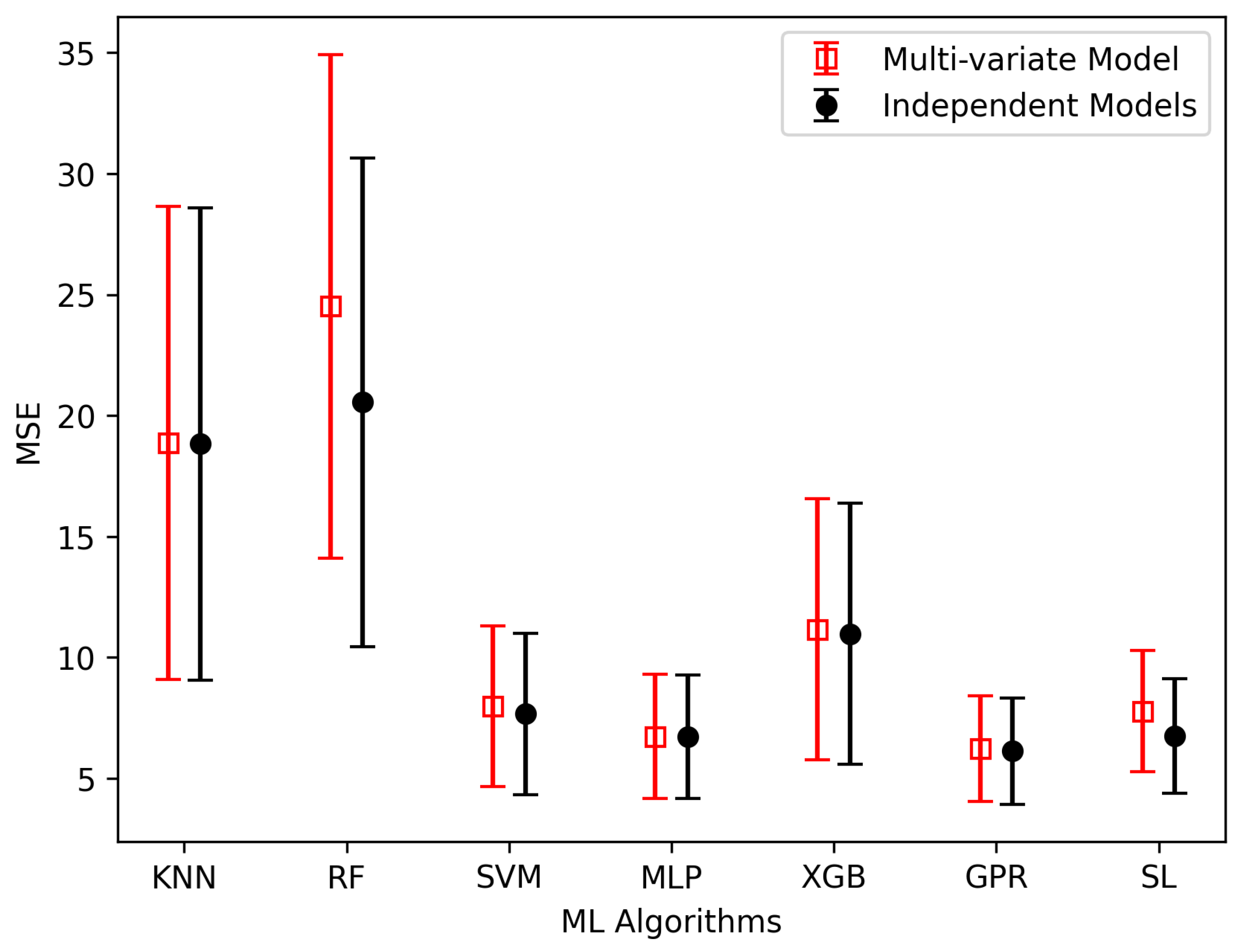
| KNN | 9.09 ± 2.97 | 9.09 ± 2.97 | 2.92 ± 1.46 | 2.90 ± 1.46 | 18.86 ± 9.81 | 18.83 ± 9.81 |
| RF | 10.20 ± 4.11 | 8.90 ± 3.21 | 3.76 ± 1.53 | 3.21 ± 1.48 | 24.52 ± 10.45 | 20.55 ± 10.14 |
| SVM | 6.81 ± 4.26 | 6.80 ± 4.25 | 1.28 ± 0.52 | 1.24 ± 0.51 | 7.96 ± 3.35 | 7.66 ± 3.33 |
| MLP | 8.36 ± 3.21 | 8.36 ± 3.21 | 1.08 ± 0.40 | 1.08 ± 0.40 | 6.72 ± 2.59 | 6.71 ± 2.56 |
| XGB | 3.99 ± 0.96 | 3.95 ± 1.09 | 1.80 ± 0.83 | 1.80 ± 0.83 | 11.15 ± 5.42 | 10.97 ± 5.41 |
| GPR | 4.13 ± 1.45 | 4.13 ± 1.45 | 1.04 ± 0.35 | 1.04 ± 0.35 | 6.32 ± 2.21 | 6.22 ± 2.20 |
| SL | 5.05 ± 1.76 | 4.00 ± 1.20 | 1.25 ± 0.40 | 1.11 ± 0.38 | 7.77 ± 2.53 | 6.75 ± 2.38 |
Disclaimer/Publisher’s Note: The statements, opinions and data contained in all publications are solely those of the individual author(s) and contributor(s) and not of MDPI and/or the editor(s). MDPI and/or the editor(s) disclaim responsibility for any injury to people or property resulting from any ideas, methods, instructions or products referred to in the content. |
© 2024 by the authors. Licensee MDPI, Basel, Switzerland. This article is an open access article distributed under the terms and conditions of the Creative Commons Attribution (CC BY) license (https://creativecommons.org/licenses/by/4.0/).
Share and Cite
Risal, S.; Singh, N.; Yao, Y.; Sun, L.; Risal, S.; Zhu, W. Accelerating Elastic Property Prediction in Fe-C Alloys through Coupling of Molecular Dynamics and Machine Learning. Materials 2024, 17, 601. https://doi.org/10.3390/ma17030601
Risal S, Singh N, Yao Y, Sun L, Risal S, Zhu W. Accelerating Elastic Property Prediction in Fe-C Alloys through Coupling of Molecular Dynamics and Machine Learning. Materials. 2024; 17(3):601. https://doi.org/10.3390/ma17030601
Chicago/Turabian StyleRisal, Sandesh, Navdeep Singh, Yan Yao, Li Sun, Samprash Risal, and Weihang Zhu. 2024. "Accelerating Elastic Property Prediction in Fe-C Alloys through Coupling of Molecular Dynamics and Machine Learning" Materials 17, no. 3: 601. https://doi.org/10.3390/ma17030601