Figure 1.
Material in dilatation gap numerical model. Three-dimensional problem. Expansion joint geometry and local coordinate systems on connection planes, left graphics. Selected nodes on connection plane, central graphics, and on central plane, right graphics. The width of the gap is equal to 1.0 cm, upper, and 2.0 cm, lower.
Figure 2.
Deformations for scaling factor 1.0 and Cauchy stresses in MPa for total load level. The width of the gap is equal to 1.0 cm, left graphics, and 2.0 cm, right graphics. Views on connection, first and third columns, or central plane, second and fourth columns.
Figure 2.
Deformations for scaling factor 1.0 and Cauchy stresses in MPa for total load level. The width of the gap is equal to 1.0 cm, left graphics, and 2.0 cm, right graphics. Views on connection, first and third columns, or central plane, second and fourth columns.
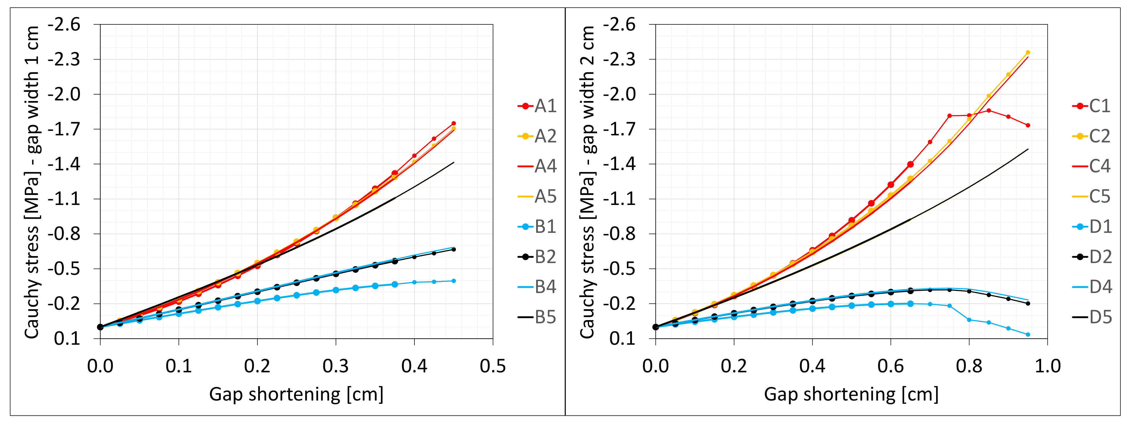
Figure 3.
Equilibrium paths for stresses σ_z in selected nodes. The width of the gap is equal to 1.0 cm, left graphic, and 2.0 cm, right.
Figure 3.
Equilibrium paths for stresses σ_z in selected nodes. The width of the gap is equal to 1.0 cm, left graphic, and 2.0 cm, right.
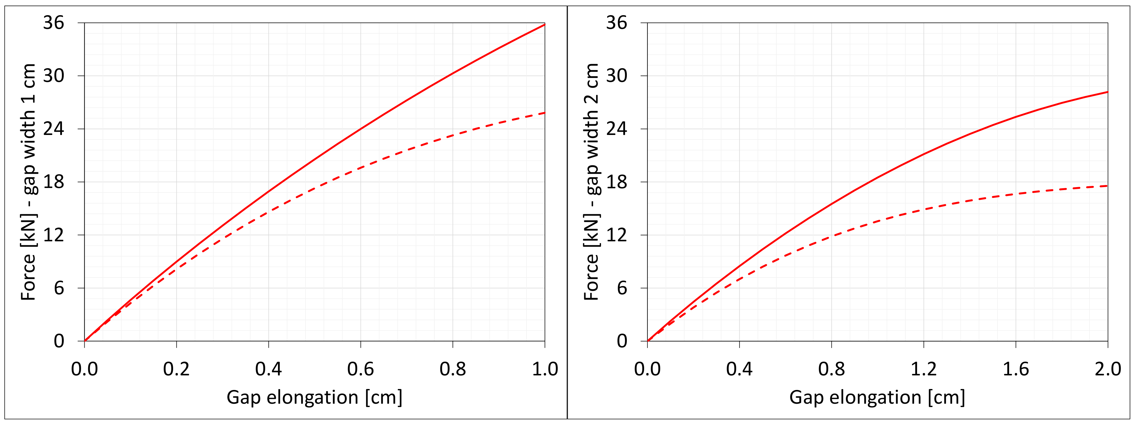
Figure 4.
Equilibrium paths for excitation force The width of the gap is equal to 1.0 cm, left graphic, and 2.0 cm, right graphic.
Figure 4.
Equilibrium paths for excitation force The width of the gap is equal to 1.0 cm, left graphic, and 2.0 cm, right graphic.
Figure 5.
Deformations for scaling factor 1.0 and Cauchy stresses in MPa for final load level. The width of the gap is equal to 1.0 cm, left graphic, and 2.0 cm, right graphic. Views on connection, first and third columns, or central plane, second and fourth columns. Details of deformation are enlarged.
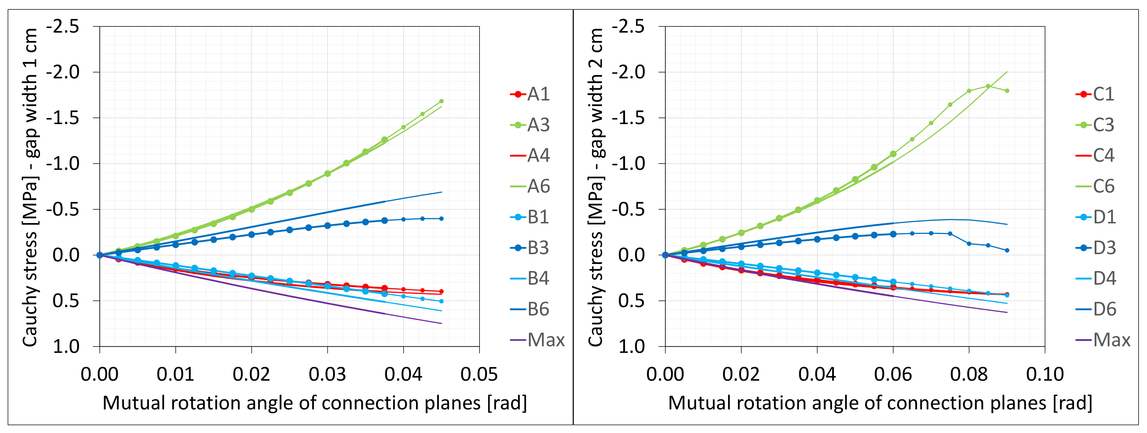
Figure 6.
Equilibrium paths for stresses in selected nodes. The width of the gap is equal to 1.0 cm, left graphic, and 2.0 cm, right graphic. Parts of charts with non-physical deformations are displayed with thin lines.
Figure 6.
Equilibrium paths for stresses in selected nodes. The width of the gap is equal to 1.0 cm, left graphic, and 2.0 cm, right graphic. Parts of charts with non-physical deformations are displayed with thin lines.
Figure 7.
Equilibrium paths for excitation force . The width of the gap is equal to 1.0 cm, left graphic, and 2.0 cm, right graphic. Parts of charts with non-physical deformations are displayed with thin lines.
Figure 7.
Equilibrium paths for excitation force . The width of the gap is equal to 1.0 cm, left graphic, and 2.0 cm, right graphic. Parts of charts with non-physical deformations are displayed with thin lines.
Figure 8.
Deformations for scaling factor 1.0 and Cauchy stresses in MPa for final load level. The width of the gap is equal to 1.0 cm, left graphics, and 2.0 cm, right graphics. Views on connection, first and third columns, or central plane, second and fourth columns.
Figure 8.
Deformations for scaling factor 1.0 and Cauchy stresses in MPa for final load level. The width of the gap is equal to 1.0 cm, left graphics, and 2.0 cm, right graphics. Views on connection, first and third columns, or central plane, second and fourth columns.
Figure 9.
Equilibrium paths for stresses in selected nodes. The gap width is equal to 1.0 cm, left graphic, and 2.0 cm, right graphic. Parts of charts with non-physical deformations are displayed with thin lines.
Figure 9.
Equilibrium paths for stresses in selected nodes. The gap width is equal to 1.0 cm, left graphic, and 2.0 cm, right graphic. Parts of charts with non-physical deformations are displayed with thin lines.
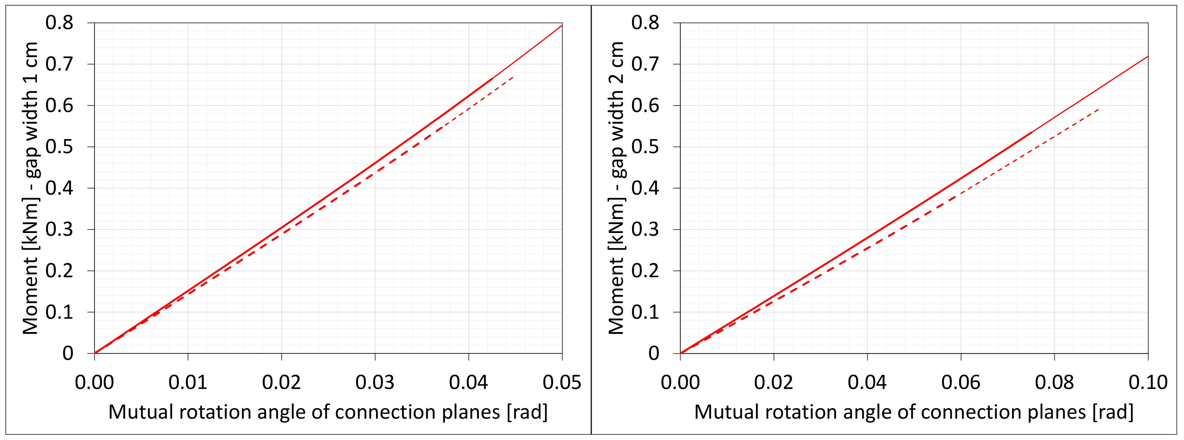
Figure 10.
Equilibrium paths for excitation moment. The gap width is equal to 1.0 cm, left graphic, and 2.0 cm, right graphic. Parts of charts with non-physical deformations are displayed with thin lines.
Figure 10.
Equilibrium paths for excitation moment. The gap width is equal to 1.0 cm, left graphic, and 2.0 cm, right graphic. Parts of charts with non-physical deformations are displayed with thin lines.
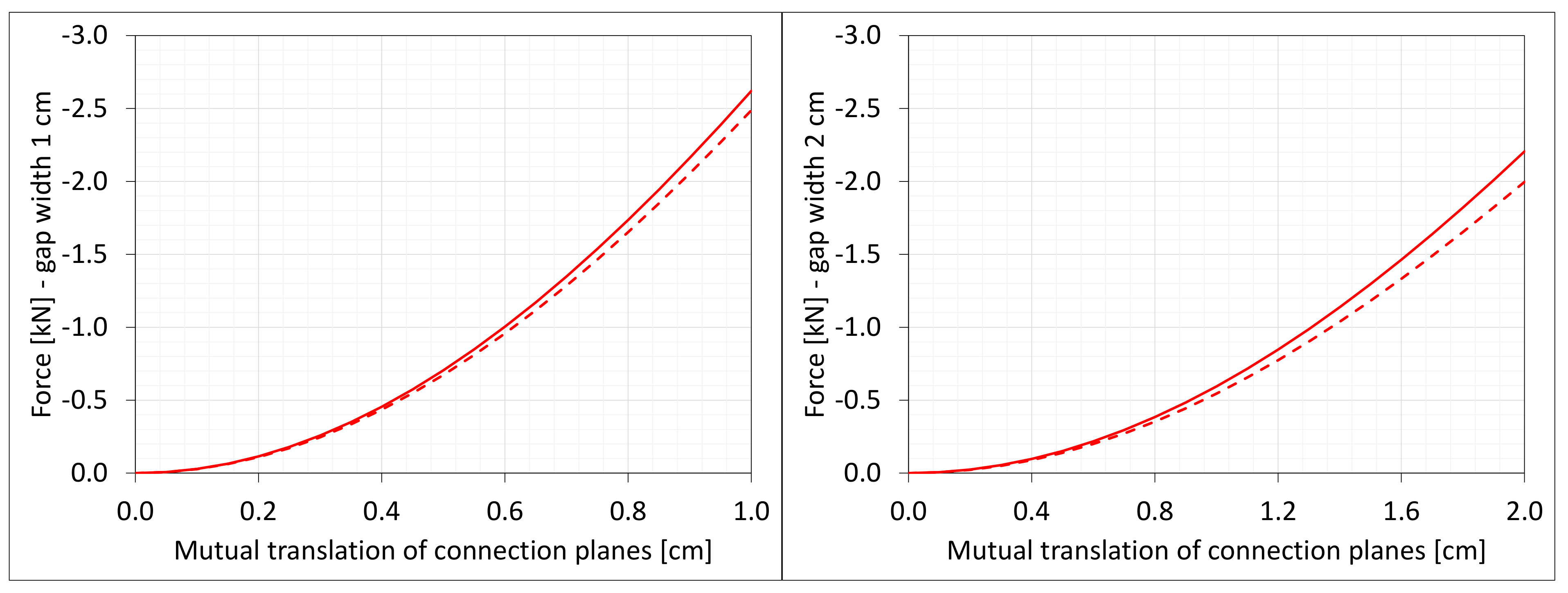
Figure 11.
Equilibrium paths for excitation force . The width of the gap is equal to 1.0 cm, left graphic, and 2.0 cm, right graphic. Parts of charts with non-physical deformations are displayed with thin lines.
Figure 11.
Equilibrium paths for excitation force . The width of the gap is equal to 1.0 cm, left graphic, and 2.0 cm, right graphic. Parts of charts with non-physical deformations are displayed with thin lines.
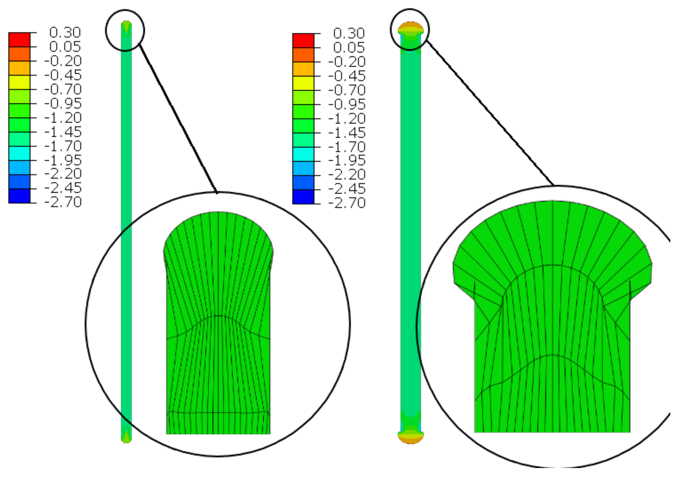
Figure 12.
Deformations for scaling factor 1.0 and Cauchy stresses in MPa for total load level. The width of the gap is equal to 1.0 cm, left graphics, and 2.0 cm, right graphic. Views on connection, first and third columns, or central plane, second and fourth columns.
Figure 12.
Deformations for scaling factor 1.0 and Cauchy stresses in MPa for total load level. The width of the gap is equal to 1.0 cm, left graphics, and 2.0 cm, right graphic. Views on connection, first and third columns, or central plane, second and fourth columns.
Figure 13.
Equilibrium paths for stresses in selected nodes. The width of the gap is equal to 1.0 cm, left graphic, and 2.0 cm, right graphic.
Figure 13.
Equilibrium paths for stresses in selected nodes. The width of the gap is equal to 1.0 cm, left graphic, and 2.0 cm, right graphic.
Figure 14.
Equilibrium paths for shear force . The width of the gap is equal to 1.0 cm, left graphic, and 2.0 cm, right graphic.
Figure 14.
Equilibrium paths for shear force . The width of the gap is equal to 1.0 cm, left graphic, and 2.0 cm, right graphic.
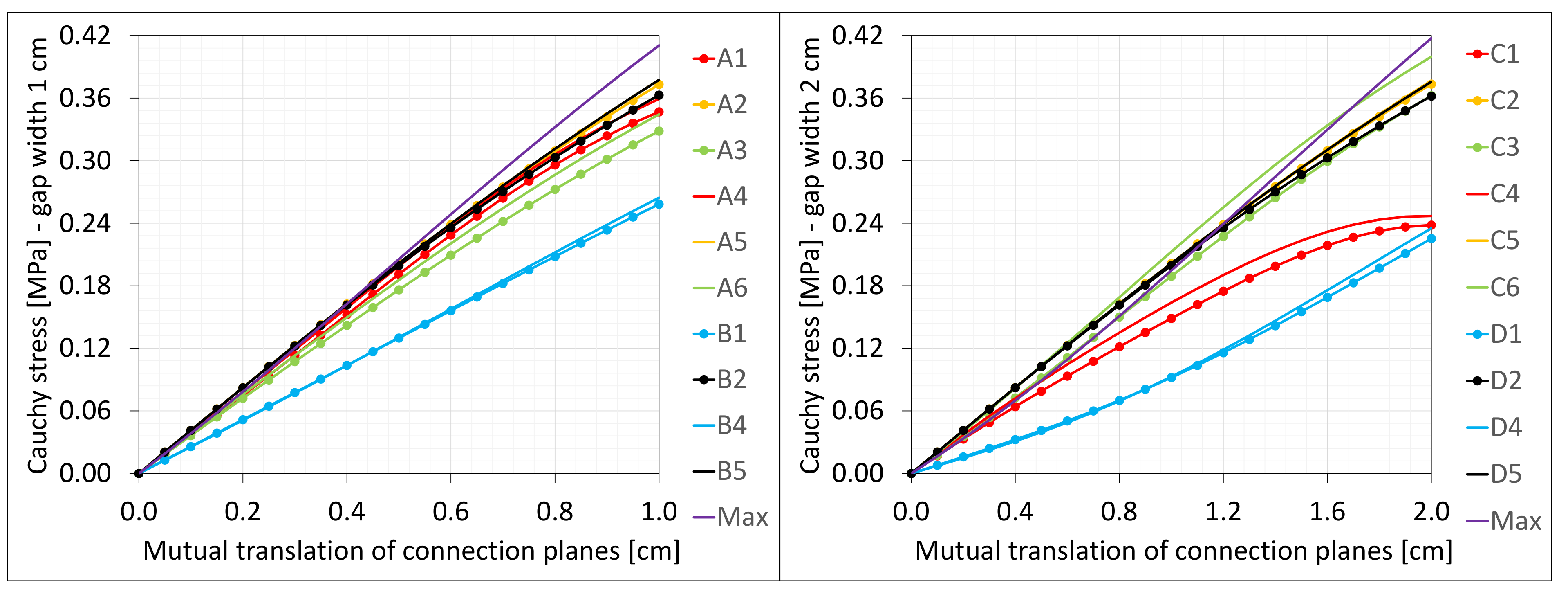
Figure 15.
Equilibrium paths for axial force . The width of the gap is equal to 1.0 cm, left graphic, and 2.0 cm, right graphic.
Figure 15.
Equilibrium paths for axial force . The width of the gap is equal to 1.0 cm, left graphic, and 2.0 cm, right graphic.
Figure 16.
Material in dilatation gap numerical model. Plane strain problem. Expansion joint geometry and local coordinate systems on connection planes, first and third graphics. Selected nodes on connection and central plane, second and fourth graphics. The width of the gap is equal to 1.0 cm, left, and 2.0 cm, right.
Figure 17.
Deformations for scaling factor 1.0 and Cauchy stresses in MPa for total load level. The width of the gap is equal to 1.0 cm, left graphic, and 2.0 cm, right graphic.
Figure 17.
Deformations for scaling factor 1.0 and Cauchy stresses in MPa for total load level. The width of the gap is equal to 1.0 cm, left graphic, and 2.0 cm, right graphic.
Figure 18.
Equilibrium paths for stresses
in selected nodes. The width of the gap is equal to 1.0 cm, left graphic, and 2.0 cm, right graphic. Plane strain models, solid lines; and 3D models, dashed lines (curves from
Figure 3).
Figure 18.
Equilibrium paths for stresses
in selected nodes. The width of the gap is equal to 1.0 cm, left graphic, and 2.0 cm, right graphic. Plane strain models, solid lines; and 3D models, dashed lines (curves from
Figure 3).
Figure 19.
Equilibrium paths for excitation force
. The width of the gap is equal to 1.0 cm, left graphic, and 2.0 cm, right graphic. Plane strain models, solid lines; and 3D models, dashed lines (curves from
Figure 4).
Figure 19.
Equilibrium paths for excitation force
. The width of the gap is equal to 1.0 cm, left graphic, and 2.0 cm, right graphic. Plane strain models, solid lines; and 3D models, dashed lines (curves from
Figure 4).
Figure 20.
Deformations for scaling factor 1.0 and Cauchy stresses in MPa for total load level. The width of the gap is equal to 1.0 cm, left graphic, and 2.0 cm, right graphic. Details of deformation are enlarged.
Figure 20.
Deformations for scaling factor 1.0 and Cauchy stresses in MPa for total load level. The width of the gap is equal to 1.0 cm, left graphic, and 2.0 cm, right graphic. Details of deformation are enlarged.
Figure 21.
Equilibrium paths for stresses
in selected nodes. The width of the gap is equal to 1.0 cm, left graphic, and 2.0 cm, right graphic. Plane strain models, solid lines; and 3D models, dashed lines (curves from
Figure 6). Parts of charts with non-physical deformations are displayed with thin lines.
Figure 22.
Equilibrium paths for excitation force
The width of the gap is equal to 1.0 cm, left graphic, and 2.0 cm, right. Plane strain models, solid lines; and 3D models, dashed lines (curves from
Figure 7). Parts of charts with non-physical de-formations are displayed with thin lines.
Figure 22.
Equilibrium paths for excitation force
The width of the gap is equal to 1.0 cm, left graphic, and 2.0 cm, right. Plane strain models, solid lines; and 3D models, dashed lines (curves from
Figure 7). Parts of charts with non-physical de-formations are displayed with thin lines.
Figure 23.
Deformations for scaling factor 1.0 and Cauchy stresses in MPa for total load level. The width of the gap is equal to 1.0 cm, left graphic, and 2.0 cm, right graphic.
Figure 23.
Deformations for scaling factor 1.0 and Cauchy stresses in MPa for total load level. The width of the gap is equal to 1.0 cm, left graphic, and 2.0 cm, right graphic.
Figure 24.
Equilibrium paths for stresses
in selected nodes. The width of the gap is equal to 1.0 cm, left graphic, and 2.0 cm, right graphic. Plane strain models, solid lines; and 3D models, dashed lines (curves from
Figure 9). Parts of charts with non-physical deformations are displayed with thin lines.
Figure 25.
Equilibrium paths for excitation moment
. The width of the gap is equal to 1.0 cm, left graphic, and 2.0 cm, right graphic. Plane strain models, solid lines; and 3D models, dashed lines (curves from
Figure 10). Parts of charts with non-physical deformations are displayed with thin lines.
Figure 25.
Equilibrium paths for excitation moment
. The width of the gap is equal to 1.0 cm, left graphic, and 2.0 cm, right graphic. Plane strain models, solid lines; and 3D models, dashed lines (curves from
Figure 10). Parts of charts with non-physical deformations are displayed with thin lines.
Figure 26.
Equilibrium paths for axial force
. The width of the gap is equal to 1.0 cm, left graphic, and 2.0 cm, right graphic. Plane strain models, solid lines; and 3D models, dashed lines (curves from
Figure 11). Parts of charts with non-physical deformations are displayed with thin lines.
Figure 26.
Equilibrium paths for axial force
. The width of the gap is equal to 1.0 cm, left graphic, and 2.0 cm, right graphic. Plane strain models, solid lines; and 3D models, dashed lines (curves from
Figure 11). Parts of charts with non-physical deformations are displayed with thin lines.
Figure 27.
Deformations for scaling factor 1.0 and Cauchy stresses in MPa for total load level. The width of the gap is equal to 1.0 cm, left graphic, and 2.0 cm, right graphic.
Figure 27.
Deformations for scaling factor 1.0 and Cauchy stresses in MPa for total load level. The width of the gap is equal to 1.0 cm, left graphic, and 2.0 cm, right graphic.
Figure 28.
Equilibrium paths for stresses
in selected nodes. The width of the gap is equal to 1.0 cm, left graphic, and 2.0 cm, right graphic. Plane strain models, solid lines; and 3D models, dashed lines (curves from
Figure 13).
Figure 28.
Equilibrium paths for stresses
in selected nodes. The width of the gap is equal to 1.0 cm, left graphic, and 2.0 cm, right graphic. Plane strain models, solid lines; and 3D models, dashed lines (curves from
Figure 13).
Figure 29.
Equilibrium paths for shear force
. The width of the gap is equal to 1.0 cm, left graphic, and 2.0 cm, right graphic. Plane strain models, solid lines; and 3D models, dashed lines (curves from
Figure 14).
Figure 29.
Equilibrium paths for shear force
. The width of the gap is equal to 1.0 cm, left graphic, and 2.0 cm, right graphic. Plane strain models, solid lines; and 3D models, dashed lines (curves from
Figure 14).
Figure 30.
Equilibrium paths for axial force
. The width of the gap is equal to 1.0 cm, left graphic, and 2.0 cm, right graphic. Plane strain models, solid lines; and 3D models, dashed lines (curves from
Figure 15).
Figure 30.
Equilibrium paths for axial force
. The width of the gap is equal to 1.0 cm, left graphic, and 2.0 cm, right graphic. Plane strain models, solid lines; and 3D models, dashed lines (curves from
Figure 15).
Table 1.
Components of tested resin.
Table 1.
Components of tested resin.
| Parameter | Component A | Component B |
|---|
| Description | Polyurethane base | Water |
| Form | Liquid | Liquid |
| pH | Undetermined | 7 |
| Density | from 1.04 to 1.16 kg/dm3 | ca. 1.00 kg/dm3 |
| Viscosity | <350 mPas | ca. 1.00 mPas |
Table 2.
Properties of tested resin.
Table 2.
Properties of tested resin.
| Property | Value |
|---|
| Viscosity | <200 mPas |
| Foam factor | >3 |
| Tensile strength | approx. 1.3 MPa |
| Elongation at break | approx. 160% |
Table 3.
Material coefficients.
Table 3.
Material coefficients.
| | | | | | | | |
|---|
| [-] | [kPa] | [kPa] | [-] | [-] | [MPa−1] | [MPa−1] | [kPa] | [kPa] |
| 2 | 410.2 | 3.306 | 1.218 | −2.883 | 1.036 | 0.000 | 413.5 | 1930 |


