
Hybrid Data-Driven Deep Learning Framework for Material Mechanical Properties Prediction with the Focus on Dual-Phase Steel Microstructures

 ,
,  , and
, and
Abstract
:1. Introduction
2. Data Generation
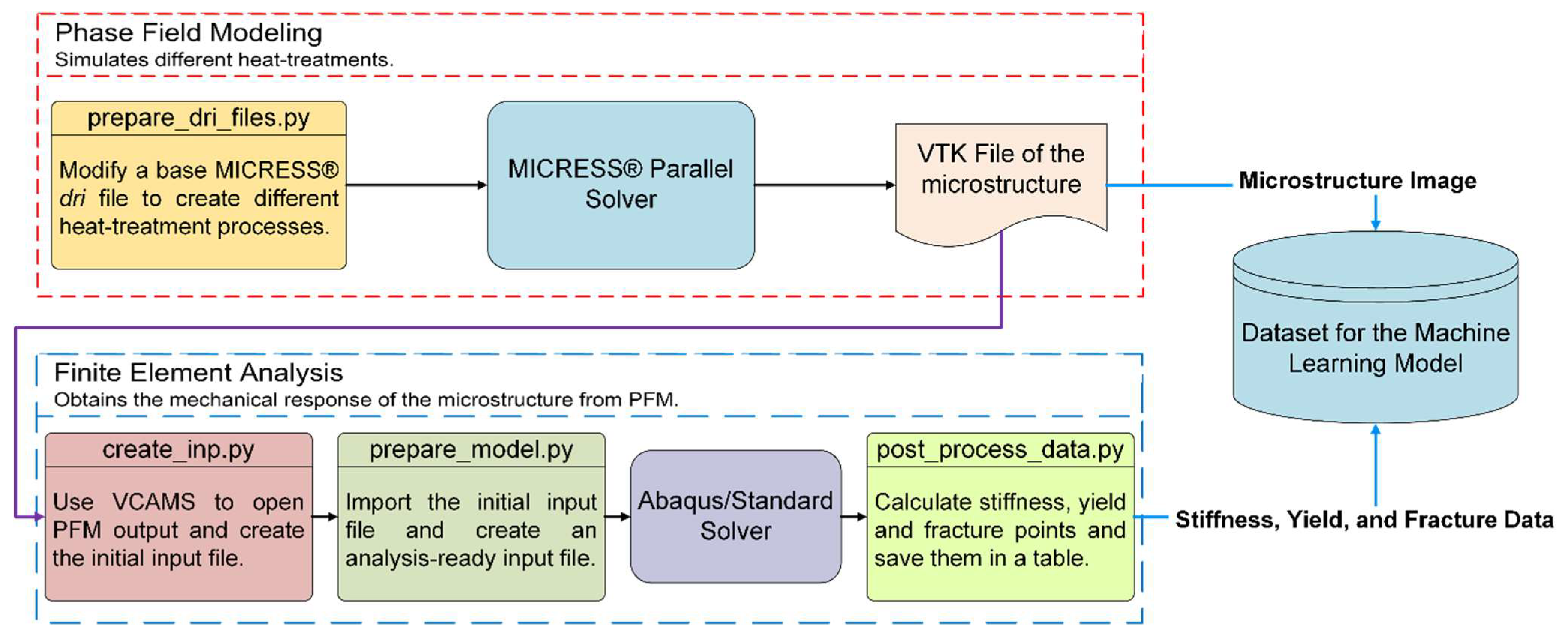
2.1. Overview
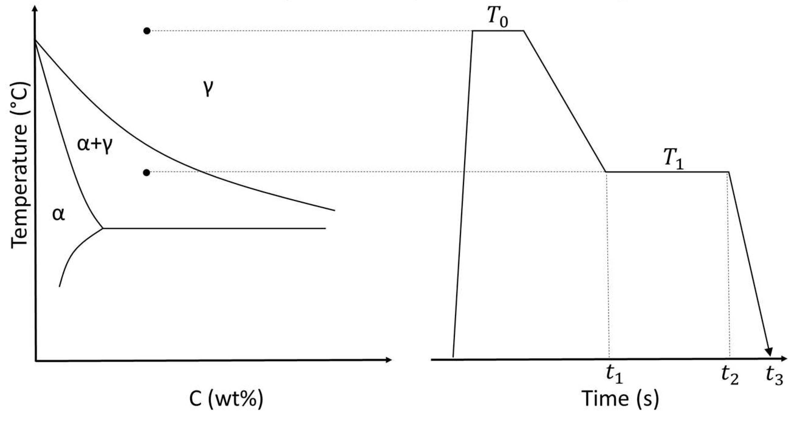
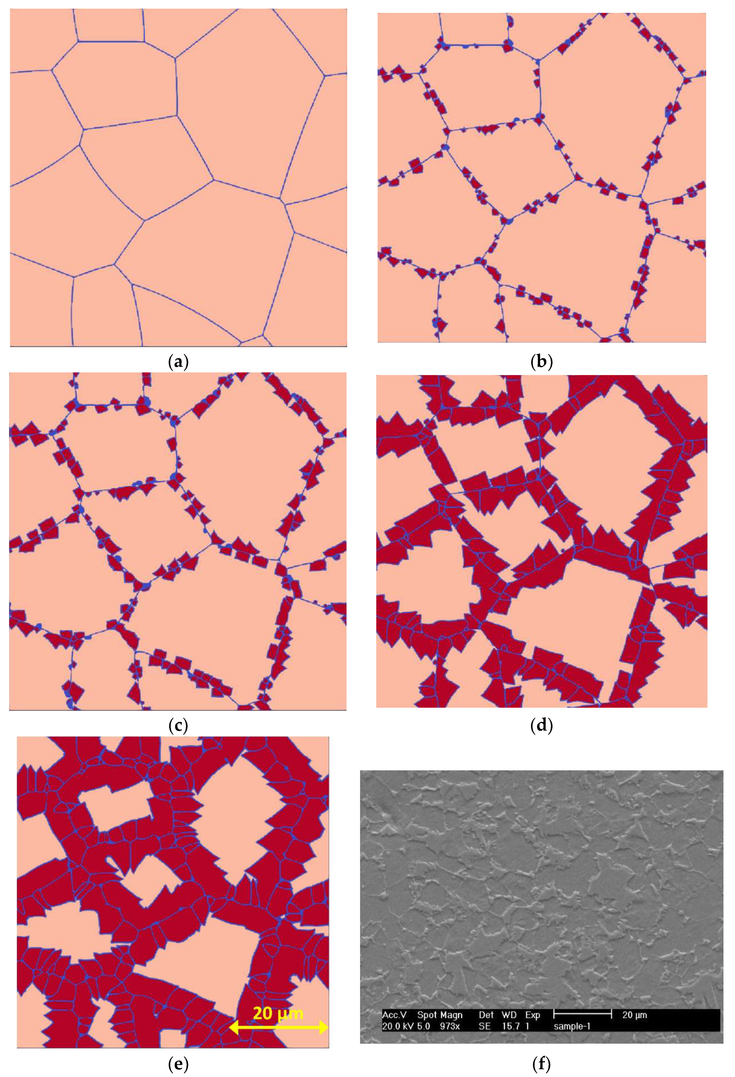
2.2. Multiphase Field Simulation
2.2.1. Basic Theory
2.2.2. Validation of PF Simulations
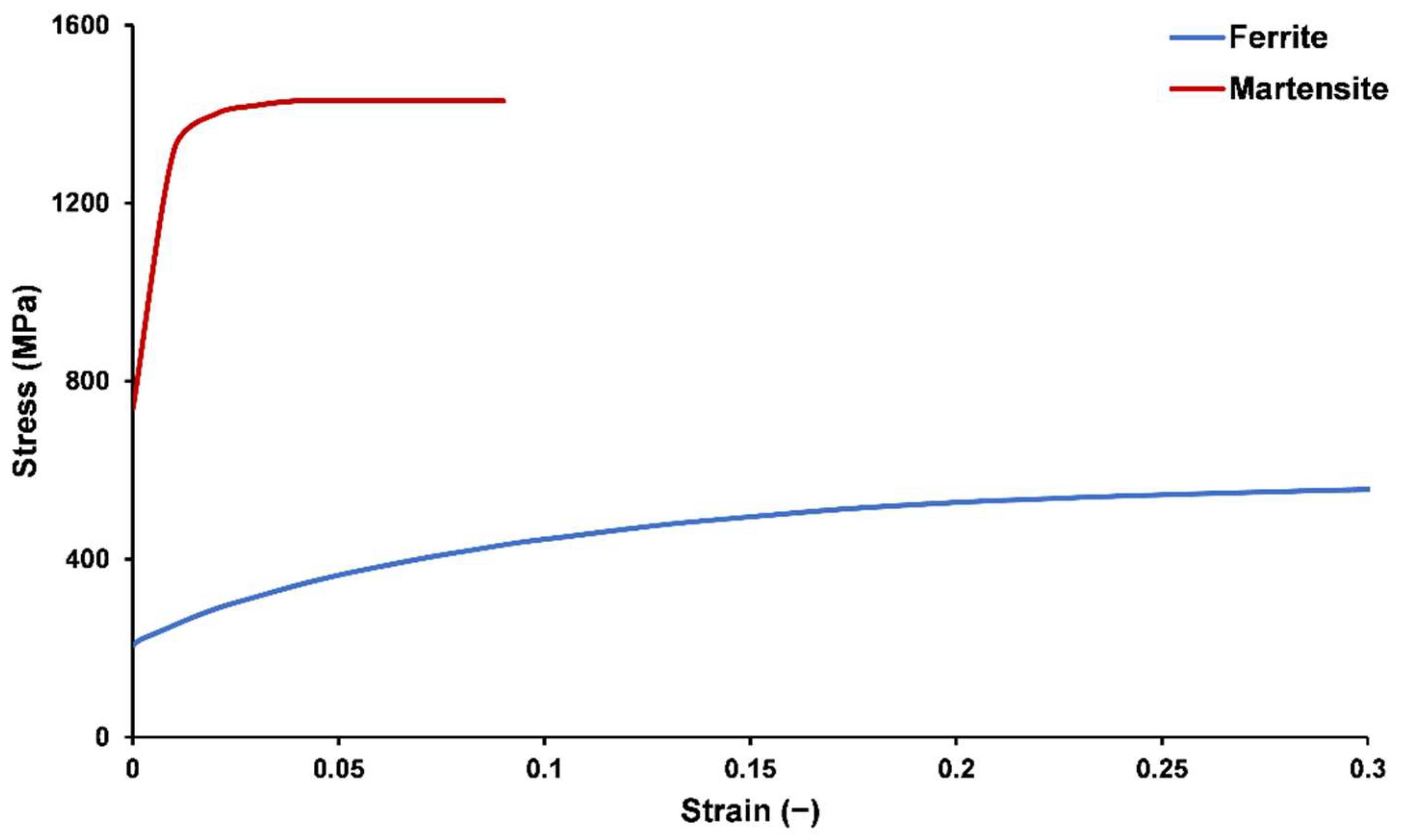
2.3. FEM Simulation
2.3.1. FEA Parameters
2.3.2. Validation of the FE Simulation
2.4. Data Pipelines
2.4.1. PFM Data Pipeline
2.4.2. FEA Data Pipeline
3. Deep Learning Approaches
3.1. Introduction and Overview
3.2. VGG16
3.3. ResNet50 (Deep Residual Learning)
3.4. Study of Hyper Parameters
3.4.1. Learning Rate (lr)
3.4.2. Dense Layers
3.4.3. Regression Ensemble Learning Method
3.5. Models’ Performance Analysis
4. Results and Discussion
5. Conclusions
Author Contributions
Funding
Institutional Review Board Statement
Informed Consent Statement
Data Availability Statement
Conflicts of Interest
References
- Rana, R.; Singh, S.B. (Eds.) Automotive Steels: Design, Metallurgy, Processing and Applications; Woodhead Publishing Series in Metals and Surface Engineering; Elsevier/Woodhead Publishing: Amsterdam, The Netherlands; Boston, MA, USA; Heidelberg, Germany, 2017; ISBN 978-0-08-100653-5. [Google Scholar]
- Cheloee Darabi, A.; Kadkhodapour, J.; Pourkamali Anaraki, A.; Khoshbin, M.; Alaie, A.; Schmauder, S. Micromechanical Modeling of Damage Mechanisms in Dual-Phase Steel under Different Stress States. Eng. Fract. Mech. 2021, 243, 107520. [Google Scholar] [CrossRef]
- Rudnizki, J.; Böttger, B.; Prahl, U.; Bleck, W. Phase-Field Modeling of Austenite Formation from a Ferrite plus Pearlite Microstructure during Annealing of Cold-Rolled Dual-Phase Steel. Metall. Mater. Trans. A 2011, 42, 2516–2525. [Google Scholar] [CrossRef]
- Zhu, B.; Militzer, M. Phase-Field Modeling for Intercritical Annealing of a Dual-Phase Steel. Metall. Mater. Trans. A 2015, 46, 1073–1084. [Google Scholar] [CrossRef]
- Rastgordani, S.; Ch Darabi, A.; Kadkhodapour, J.; Hamzeloo, S.R.; Khoshbin, M.; Schmauder, S.; Mola, J. Damage Characterization of Heat-Treated Titanium Bio-Alloy (Ti–6Al–4V) Based on Micromechanical Modeling. Surf. Topogr. Metrol. Prop. 2020, 8, 045016. [Google Scholar] [CrossRef]
- Yamanaka, A. Prediction of 3D Microstructure and Plastic Deformation Behavior in Dual-Phase Steel Using Multi-Phase Field and Crystal Plasticity FFT Methods. Key Eng. Mater. 2015, 651–653, 570–574. [Google Scholar] [CrossRef]
- Laschet, G.; Apel, M. Thermo-Elastic Homogenization of 3-D Steel Microstructure Simulated by the Phase-Field Method. Steel Res. Int. 2010, 81, 637–643. [Google Scholar] [CrossRef]
- Guo, K.; Yang, Z.; Yu, C.-H.; Buehler, M.J. Artificial Intelligence and Machine Learning in Design of Mechanical Materials. Mater. Horiz. 2021, 8, 1153–1172. [Google Scholar] [CrossRef]
- Liu, R.; Yabansu, Y.C.; Agrawal, A.; Kalidindi, S.R.; Choudhary, A.N. Machine Learning Approaches for Elastic Localization Linkages in High-Contrast Composite Materials. Integr. Mater. Manuf. Innov. 2015, 4, 192–208. [Google Scholar] [CrossRef] [Green Version]
- Hertel, L.; Collado, J.; Sadowski, P.; Ott, J.; Baldi, P. Sherpa: Robust Hyperparameter Optimization for Machine Learning. SoftwareX 2020, 12, 100591. [Google Scholar] [CrossRef]
- Chowdhury, A.; Kautz, E.; Yener, B.; Lewis, D. Image Driven Machine Learning Methods for Microstructure Recognition. Comput. Mater. Sci. 2016, 123, 176–187. [Google Scholar] [CrossRef]
- Khorrami, M.S.; Mianroodi, J.R.; Siboni, N.H.; Goyal, P.; Svendsen, B.; Benner, P.; Raabe, D. An Artificial Neural Network for Surrogate Modeling of Stress Fields in Viscoplastic Polycrystalline Materials. arXiv 2022, arXiv:2208.13490. [Google Scholar] [CrossRef]
- Yang, Z.; Yabansu, Y.C.; Al-Bahrani, R.; Liao, W.; Choudhary, A.N.; Kalidindi, S.R.; Agrawal, A. Deep Learning Approaches for Mining Structure-Property Linkages in High Contrast Composites from Simulation Datasets. Comput. Mater. Sci. 2018, 151, 278–287. [Google Scholar] [CrossRef]
- Peivaste, I.; Siboni, N.H.; Alahyarizadeh, G.; Ghaderi, R.; Svendsen, B.; Raabe, D.; Mianroodi, J.R. Accelerating Phase-Field-Based Simulation via Machine Learning. arXiv 2022, arXiv:2205.02121. [Google Scholar] [CrossRef]
- Li, X.; Liu, Z.; Cui, S.; Luo, C.; Li, C.; Zhuang, Z. Predicting the Effective Mechanical Property of Heterogeneous Materials by Image Based Modeling and Deep Learning. Comput. Methods Appl. Mech. Eng. 2019, 347, 735–753. [Google Scholar] [CrossRef] [Green Version]
- Li, Y.; Hu, S.; Sun, X.; Stan, M. A Review: Applications of the Phase Field Method in Predicting Microstructure and Property Evolution of Irradiated Nuclear Materials. npj Comput. Mater. 2017, 3, 16. [Google Scholar] [CrossRef] [Green Version]
- Gu, G.X.; Chen, C.-T.; Buehler, M.J. De Novo Composite Design Based on Machine Learning Algorithm. Extreme Mech. Lett. 2018, 18, 19–28. [Google Scholar] [CrossRef]
- Peivaste, I.; Siboni, N.H.; Alahyarizadeh, G.; Ghaderi, R.; Svendsen, B.; Raabe, D.; Mianroodi, J.R. Machine-Learning-Based Surrogate Modeling of Microstructure Evolution Using Phase-Field. Comput. Mater. Sci. 2022, 214, 111750. [Google Scholar] [CrossRef]
- Jung, J.; Na, J.; Park, H.K.; Park, J.M.; Kim, G.; Lee, S.; Kim, H.S. Super-Resolving Material Microstructure Image via Deep Learning for Microstructure Characterization and Mechanical Behavior Analysis. Npj Comput. Mater. 2021, 7, 96. [Google Scholar] [CrossRef]
- Rabbani, A.; Babaei, M.; Shams, R.; Da Wang, Y.; Chung, T. DeePore: A Deep Learning Workflow for Rapid and Comprehensive Characterization of Porous Materials. Adv. Water Resour. 2020, 146, 103787. [Google Scholar] [CrossRef]
- Kautz, E.; Ma, W.; Baskaran, A.; Chowdhury, A.; Joshi, V.; Yener, B.; Lewis, D. Image-Driven Discriminative and Generative Methods for Establishing Microstructure-Processing Relationships Relevant to Nuclear Fuel Processing Pipelines. Microsc. Microanal. 2021, 27, 2128–2130. [Google Scholar] [CrossRef]
- Banerjee, D.; Sparks, T.D. Comparing Transfer Learning to Feature Optimization in Microstructure Classification. iScience 2022, 25, 103774. [Google Scholar] [CrossRef] [PubMed]
- Tsutsui, K.; Matsumoto, K.; Maeda, M.; Takatsu, T.; Moriguchi, K.; Hayashi, K.; Morito, S.; Terasaki, H. Mixing Effects of SEM Imaging Conditions on Convolutional Neural Network-Based Low-Carbon Steel Classification. Mater. Today Commun. 2022, 32, 104062. [Google Scholar] [CrossRef]
- Steinbach, I.; Pezzolla, F. A Generalized Field Method for Multiphase Transformations Using Interface Fields. Phys. Nonlinear Phenom. 1999, 134, 385–393. [Google Scholar] [CrossRef]
- Eiken, J.; Böttger, B.; Steinbach, I. Multiphase-Field Approach for Multicomponent Alloys with Extrapolation Scheme for Numerical Application. Phys. Rev. E 2006, 73, 066122. [Google Scholar] [CrossRef] [PubMed]
- ACCESS, e.V. MICRESS Microstructure Simulation Software Manual, Version 7.0. Available online: https://micress.rwth-aachen.de/download.html#manuals (accessed on 21 November 2022).
- Kozeschnik, E. MatCalc Software, version 6.03 (rel 1.000); Materials Center Leoben Forschungsgesellschaft; Materials Cener Leoben MatCalc: Leoben, Austria, 2020.
- Krauss, G. Quench and Tempered Martensitic Steels. In Comprehensive Materials Processing; Elsevier: Amsterdam, The Netherlands, 2014; pp. 363–378. ISBN 978-0-08-096533-8. [Google Scholar]
- Steinbach, I.; Pezzolla, F.; Nestler, B.; Seeßelberg, M.; Prieler, R.; Schmitz, G.J.; Rezende, J.L.L. A Phase Field Concept for Multiphase Systems. Phys. Nonlinear Phenom. 1996, 94, 135–147. [Google Scholar] [CrossRef]
- Bréchet., Y. (Ed.) Solid-Solid Phase Transformations in Inorganic Materials; Solid State Phenomena; Trans Tech Publications: Durnten-Zuerich, Switzerland; Enfield, NH, USA, 2011; ISBN 978-3-03785-143-2. [Google Scholar]
- Azizi-Alizamini, H.; Militzer, M. Phase Field Modelling of Austenite Formation from Ultrafine Ferrite–Carbide Aggregates in Fe–C. Int. J. Mater. Res. 2010, 101, 534–541. [Google Scholar] [CrossRef]
- Steinbach, I.; Apel, M. The Influence of Lattice Strain on Pearlite Formation in Fe–C. Acta Mater. 2007, 55, 4817–4822. [Google Scholar] [CrossRef]
- Pierman, A.-P.; Bouaziz, O.; Pardoen, T.; Jacques, P.J.; Brassart, L. The Influence of Microstructure and Composition on the Plastic Behaviour of Dual-Phase Steels. Acta Mater. 2014, 73, 298–311. [Google Scholar] [CrossRef]
- Alibeyki, M.; Mirzadeh, H.; Najafi, M.; Kalhor, A. Modification of Rule of Mixtures for Estimation of the Mechanical Properties of Dual-Phase Steels. J. Mater. Eng. Perform. 2017, 26, 2683–2688. [Google Scholar] [CrossRef]
- Ch.Darabi, A.; Chamani, H.R.; Kadkhodapour, J.; Anaraki, A.P.; Alaie, A.; Ayatollahi, M.R. Micromechanical Analysis of Two Heat-Treated Dual Phase Steels: DP800 and DP980. Mech. Mater. 2017, 110, 68–83. [Google Scholar] [CrossRef]
- Ramprasad, R.; Batra, R.; Pilania, G.; Mannodi-Kanakkithodi, A.; Kim, C. Machine Learning in Materials Informatics: Recent Applications and Prospects. Npj Comput. Mater. 2017, 3, 54. [Google Scholar] [CrossRef] [Green Version]
- Azimi, S.M.; Britz, D.; Engstler, M.; Fritz, M.; Mücklich, F. Advanced Steel Microstructural Classification by Deep Learning Methods. Sci. Rep. 2018, 8, 2128. [Google Scholar] [CrossRef] [PubMed] [Green Version]
- Smokvina Hanza, S.; Marohnić, T.; Iljkić, D.; Basan, R. Artificial Neural Networks-Based Prediction of Hardness of Low-Alloy Steels Using Specific Jominy Distance. Metals 2021, 11, 714. [Google Scholar] [CrossRef]
- Agrawal, A.; Gopalakrishnan, K.; Choudhary, A. Materials Image Informatics Using Deep Learning. In Handbook on Big Data and Machine Learning in the Physical Sciences; World Scientific Publishing Co.: Singapore, 2020; pp. 205–230. [Google Scholar]
- Kwak, S.; Kim, J.; Ding, H.; Xu, X.; Chen, R.; Guo, J.; Fu, H. Machine Learning Prediction of the Mechanical Properties of γ-TiAl Alloys Produced Using Random Forest Regression Model. J. Mater. Res. Technol. 2022, 18, 520–530. [Google Scholar] [CrossRef]
- Gajewski, J.; Golewski, P.; Sadowski, T. The Use of Neural Networks in the Analysis of Dual Adhesive Single Lap Joints Subjected to Uniaxial Tensile Test. Materials 2021, 14, 419. [Google Scholar] [CrossRef]
- Kosarac, A.; Cep, R.; Trochta, M.; Knezev, M.; Zivkovic, A.; Mladjenovic, C.; Antic, A. Thermal Behavior Modeling Based on BP Neural Network in Keras Framework for Motorized Machine Tool Spindles. Materials 2022, 15, 7782. [Google Scholar] [CrossRef]
- Valença, J.; Mukhandi, H.; Araújo, A.G.; Couceiro, M.S.; Júlio, E. Benchmarking for Strain Evaluation in CFRP Laminates Using Computer Vision: Machine Learning versus Deep Learning. Materials 2022, 15, 6310. [Google Scholar] [CrossRef]
- Azarafza, M.; Hajialilue Bonab, M.; Derakhshani, R. A Deep Learning Method for the Prediction of the Index Mechanical Properties and Strength Parameters of Marlstone. Materials 2022, 15, 6899. [Google Scholar] [CrossRef]
- Liu, H.; Motoda, H. Feature Selection for Knowledge Discovery and Data Mining; Springer: Boston, MA, USA, 1998; ISBN 978-1-4613-7604-0. [Google Scholar]
- Rasool, M.; Ismail, N.A.; Boulila, W.; Ammar, A.; Samma, H.; Yafooz, W.M.S.; Emara, A.-H.M. A Hybrid Deep Learning Model for Brain Tumour Classification. Entropy 2022, 24, 799. [Google Scholar] [CrossRef]
- Zou, F.; Shen, L.; Jie, Z.; Zhang, W.; Liu, W. A Sufficient Condition for Convergences of Adam and RMSProp. arxiv 2018, arXiv:1811.09358. [Google Scholar] [CrossRef]
- Ramstad, T.; Idowu, N.; Nardi, C.; Øren, P.-E. Relative Permeability Calculations from Two-Phase Flow Simulations Directly on Digital Images of Porous Rocks. Transp. Porous Media 2012, 94, 487–504. [Google Scholar] [CrossRef]
- Simonyan, K.; Zisserman, A. Very Deep Convolutional Networks for Large-Scale Image Recognition. arxiv 2014, arXiv:1409.1556. [Google Scholar] [CrossRef]
- Patel, A.; Cheung, L.; Khatod, N.; Matijosaitiene, I.; Arteaga, A.; Gilkey, J.W. Revealing the Unknown: Real-Time Recognition of Galápagos Snake Species Using Deep Learning. Animals 2020, 10, 806. [Google Scholar] [CrossRef] [PubMed]
- Pengtao, W. Based on Adam Optimization Algorithm: Neural Network Model for Auto Steel Performance Prediction. J. Phys. Conf. Ser. 2020, 1653, 012012. [Google Scholar] [CrossRef]
- He, K.; Zhang, X.; Ren, S.; Sun, J. Deep Residual Learning for Image Recognition. arxiv 2015, arXiv:1512.03385. [Google Scholar] [CrossRef]
- Xu, M.; Wang, S.; Guo, J.; Li, Y. Robust Structural Damage Detection Using Analysis of the CMSE Residual’s Sensitivity to Damage. Appl. Sci. 2020, 10, 2826. [Google Scholar] [CrossRef] [Green Version]
- Pedersen, M.E.H. Available online: https://github.com/Hvass-Labs/TensorFlow-Tutorials/blob/master/11_Adversarial_Examples.ipynb (accessed on 2 April 2020).
- Brownlee, J. Loss and Loss Functions for Training Deep Learning Neural Networks. Machine Learning Mastery. 23 October 2019. Available online: https://machinelearningmastery.com/loss-and-loss-functions-for-training-deep-learning-neural-networks/ (accessed on 21 November 2022).
- Ritter, C.; Wollmann, T.; Bernhard, P.; Gunkel, M.; Braun, D.M.; Lee, J.-Y.; Meiners, J.; Simon, R.; Sauter, G.; Erfle, H.; et al. Hyperparameter Optimization for Image Analysis: Application to Prostate Tissue Images and Live Cell Data of Virus-Infected Cells. Int. J. Comput. Assist. Radiol. Surg. 2019, 14, 1847–1857. [Google Scholar] [CrossRef] [PubMed]
- Hyndman, R.J.; Koehler, A.B. Another Look at Measures of Forecast Accuracy. Int. J. Forecast. 2006, 22, 679–688. [Google Scholar] [CrossRef] [Green Version]
- Medghalchi, S.; Kusche, C.F.; Karimi, E.; Kerzel, U.; Korte-Kerzel, S. Damage Analysis in Dual-Phase Steel Using Deep Learning: Transfer from Uniaxial to Biaxial Straining Conditions by Image Data Augmentation. JOM 2020, 72, 4420–4430. [Google Scholar] [CrossRef]
- Bengio, Y. Practical Recommendations for Gradient-Based Training of Deep Architectures. arxiv 2012, arXiv:1206.5533. [Google Scholar] [CrossRef]
- Ibrahim, M.M. The Design of an Innovative Automatic Computational Method for Generating Geometric Islamic Visual Art with Aesthetic Beauty. University of Bedfordshire, 2021. Available online: https://uobrep.openrepository.com/handle/10547/625007 (accessed on 21 November 2022).
- Brownlee, J. Data Preparation for Machine Learning: Data Cleaning, Feature Selection, and Data Transforms in Python; Machine Learning Mastery: San Francisco, CA, USA, 2020; Available online: https://machinelearningmastery.com/data-preparation-for-machine-learning/ (accessed on 21 November 2022).
- Wang, Y.; Oyen, D.; Guo, W.G.; Mehta, A.; Scott, C.B.; Panda, N.; Fernández-Godino, M.G.; Srinivasan, G.; Yue, X. StressNet—Deep Learning to Predict Stress with Fracture Propagation in Brittle Materials. npj Mater. Degrad. 2021, 5, 6. [Google Scholar] [CrossRef]


| Element | C | Mn | Si | P | S | Cr | Mo | V | Cu | Co |
|---|---|---|---|---|---|---|---|---|---|---|
| wt% | 0.2 | 1.1 | 0.22 | 0.004 | 0.02 | 0.157 | 0.04 | 0.008 | 0.121 | 0.019 |
| Phase Boundary | α/γ + α | γ/α + γ | |
|---|---|---|---|
| Carbon () | Concentration (wt%) | 0.0048 | 0.365 |
| Slope (°K/wt%) | −13,972.00 | −188.80 | |
| Manganese () | Concentration (wt%) | 1.58 | 3.78 |
| Slope (°K/wt%) | −100.03 | −23.55 | |
| 0.238 | |||
| Interface | α/α | α/γ | γ/γ |
|---|---|---|---|
| Interfacial energy (J) | 7.60 × | 7.20 × | 7.60 × |
| Mobility () | 5.00 × | 2.40 × | 3.50 × |
| Yield Stress (MPa) | Ultimate Stress (MPa) | Fracture Strain (−) | |
|---|---|---|---|
| Numerical | 314.36 | 517.9 | 0.127 |
| Experimental | 323.7 | 530.1 | 0.131 |
| Parameter | Description | Values |
|---|---|---|
| Initial temperature of the microstructure. | 1250 | |
| Cooling rate between points 0 and 1. Not used directly. | −10, −5, −1 | |
| Number of seconds it takes to cool down from point 1 to point 2. | Calculated based on | |
| Temperature of the microstructure in point 1. | 1000, 1010, 1020, 1030, 1040, 1050, 1060, 1070, 1080, 1090, 1100, 1110 | |
| Holding time between points 1 and 2 in seconds. | 10, 20, 30, 60, 300, 600, 900, 1800, 3600, 7200, 10,800 | |
| Temperature of the microstructure in point 2. | Equal to | |
| Cooling rate between points 2 and 3 based on the quench media. Not used directly. | ||
| Number of seconds it takes to cool down from point 1 to point 2. | Calculated based on | |
| Room temperature. | 298 |
| Rotate 90 CC | MASE Y | MASE U | MASE F | |
| Hybrid Model Error Report (%) | Train | 10.196 | 6.681 | 11.215 |
| Test | 10.209 | 6.308 | 11.440 | |
| Rotate 90 CCW | MASE Y | MASE U | MASE F | |
| Hybrid Model Error Report (%) | Train | 10.89 | 6.502 | 12.002 |
| Test | 11.01 | 6.401 | 11.928 | |
| Random Shear | MASE Y | MASE U | MASE F | |
| Hybrid Model Error Report (%) | Train | 1.232 | 0.943 | 2.9172 |
| Test | 3.534 | 2.346 | 8.134 | |
| Flip UD | MASE Y | MASE U | MASE F | |
| Hybrid Model Error Report (%) | Train | 1.4474 | 1.0802 | 3.0451 |
| Test | 4.623 | 2.971 | 8.677 | |
| Flip LR | MASE Y | MASE U | MASE F | |
| Hybrid Model Error Report (%) | Train | 1.0306 | 0.8930 | 2.744 |
| Test | 2.692 | 2.195 | 7.025 |
| Parameter | Description | Values | VGG16 Optimized Values | ResNet50 Optimized Values |
|---|---|---|---|---|
| Epoch numbers | 200 | 200 | 200 | |
| Learning rate | 1 × 10⁻², 1 × 10⁻³, 1 × 10⁻⁴, 1 × 10⁻⁵ | 1 × 10⁻⁴ | 1 × 10⁻³ | |
| Number of filters in the convolution layer | min = 16, max = 512, step = 32 | 336 | 16 | |
(layer1) | Output size of each dense layer | min = 32, max = 1024, step = 64 | 992 | 992 |
(layer2) | - | 672 | ||
(layer3) | - | 32 |
| MASE Y | MASE U | MASE F | ||
|---|---|---|---|---|
| Resnet50 Model Error Report (%) | Train | 5.559 | 3.713 | 8.092 |
| Test | 5.465 | 3.610 | 10.448 | |
| MASE Y | MASE U | MASE F | ||
|---|---|---|---|---|
| VGG16 Model Error Report (%) | Train | 13.043 | 16.071 | 36.67 |
| Test | 11.292 | 15.001 | 41.963 | |
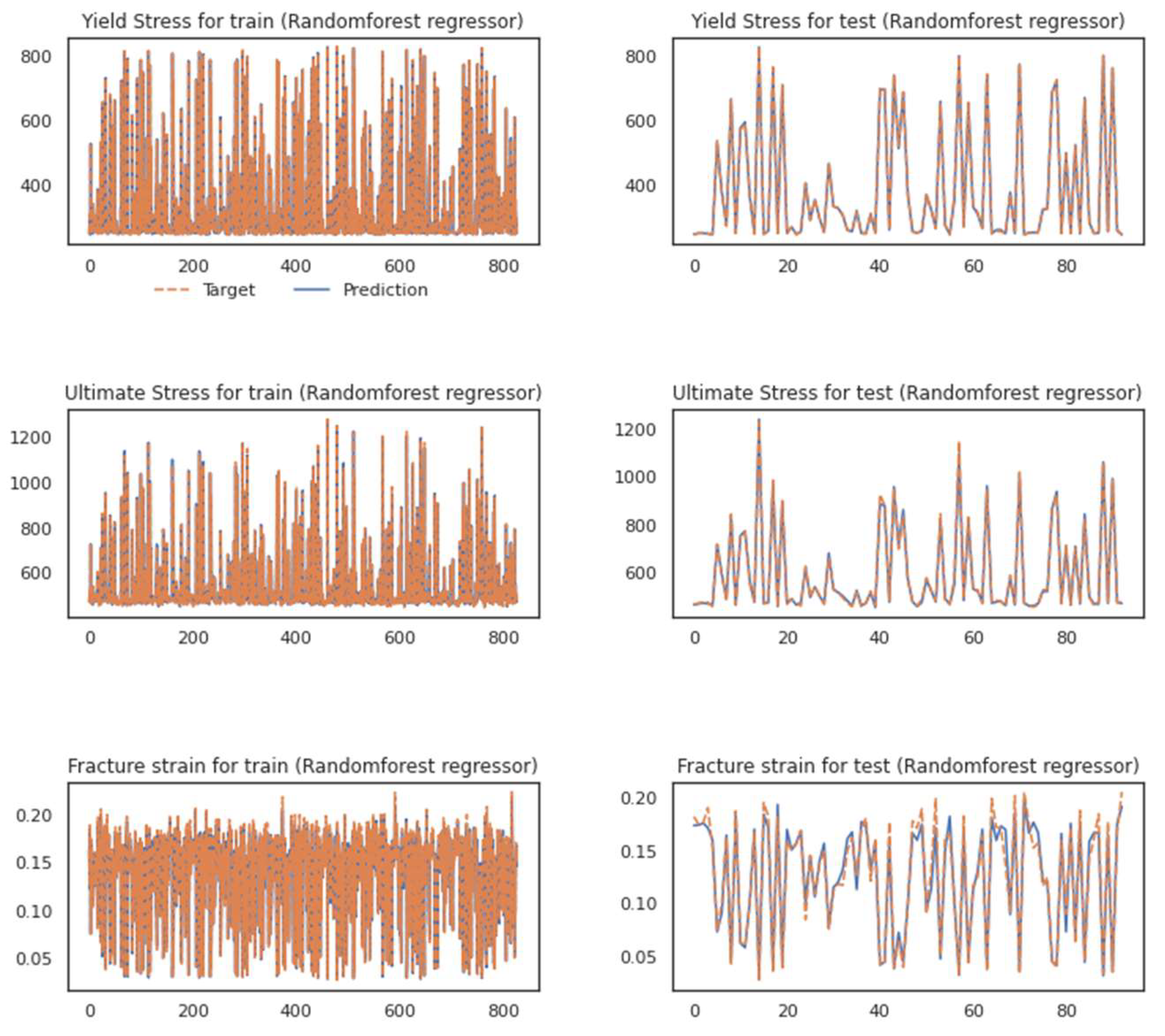
| Hybrid Model Error Report | MASE Y | MASE U | MASE F | |
|---|---|---|---|---|
| Adaboost (%) | Train | 2.532 | 1.625 | 6.323 |
| Test | 2.387 | 2.172 | 6.881 | |
| MASE Y | MASE U | MASE F | ||
| Random Forest (%) | Train | 0.386 | 0.494 | 2.432 |
| Test | 0.924 | 0.574 | 6.670 | |
Disclaimer/Publisher’s Note: The statements, opinions and data contained in all publications are solely those of the individual author(s) and contributor(s) and not of MDPI and/or the editor(s). MDPI and/or the editor(s) disclaim responsibility for any injury to people or property resulting from any ideas, methods, instructions or products referred to in the content. |
© 2023 by the authors. Licensee MDPI, Basel, Switzerland. This article is an open access article distributed under the terms and conditions of the Creative Commons Attribution (CC BY) license (https://creativecommons.org/licenses/by/4.0/).
Share and Cite
Cheloee Darabi, A.; Rastgordani, S.; Khoshbin, M.; Guski, V.; Schmauder, S. Hybrid Data-Driven Deep Learning Framework for Material Mechanical Properties Prediction with the Focus on Dual-Phase Steel Microstructures. Materials 2023, 16, 447. https://doi.org/10.3390/ma16010447
Cheloee Darabi A, Rastgordani S, Khoshbin M, Guski V, Schmauder S. Hybrid Data-Driven Deep Learning Framework for Material Mechanical Properties Prediction with the Focus on Dual-Phase Steel Microstructures. Materials. 2023; 16(1):447. https://doi.org/10.3390/ma16010447
Chicago/Turabian StyleCheloee Darabi, Ali, Shima Rastgordani, Mohammadreza Khoshbin, Vinzenz Guski, and Siegfried Schmauder. 2023. "Hybrid Data-Driven Deep Learning Framework for Material Mechanical Properties Prediction with the Focus on Dual-Phase Steel Microstructures" Materials 16, no. 1: 447. https://doi.org/10.3390/ma16010447