
Estimate of Coffin–Manson Curve Shift for the Porous Alloy AlSi9Cu3 Based on Numerical Simulations of a Porous Material Carried Out by Using the Taguchi Array


Abstract
:
1. Introduction
2. Materials and Methods
2.1. Methodology
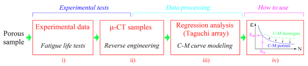
- (i)
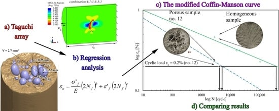
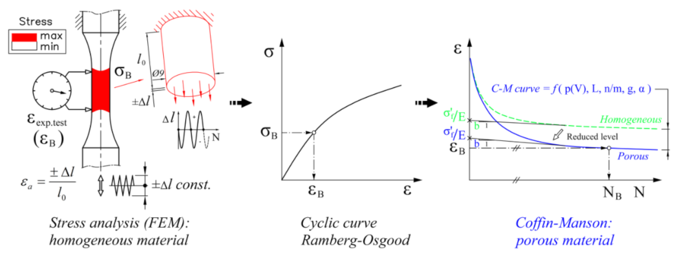
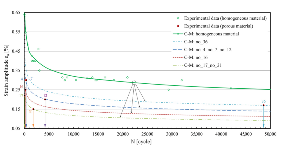
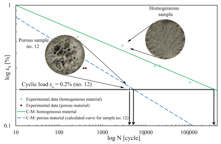
- From the experimental tests, the basic Coffin–Manson endurance curve of a homogeneous material is determined. The least-squares method is used to connect the experimental points into a uniform curve.
- (ii)
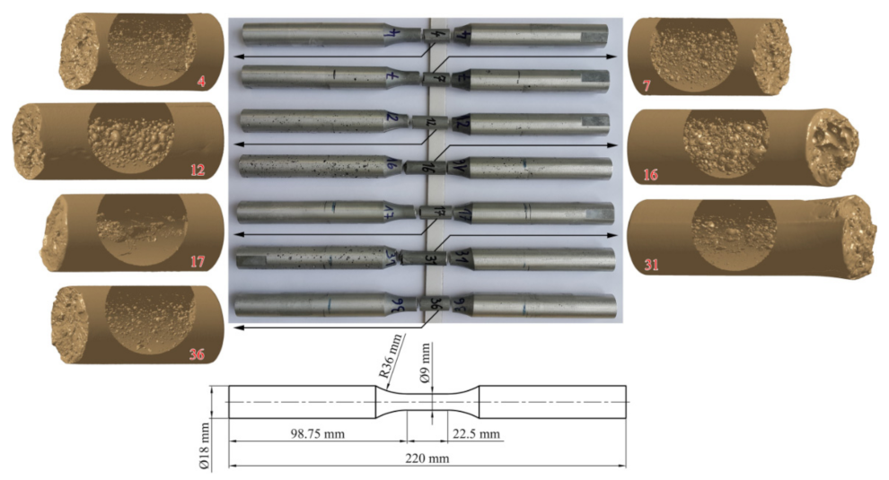
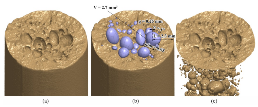
- To analyse the porosity in the alloy, the geometry of the pores is determined by using the μ-CT examination and reverse engineering based on the voxel-processing technique.
- (iii)
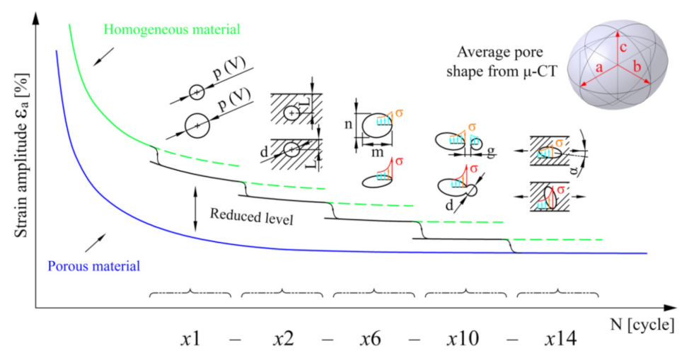
- This is followed by the most important phase, i.e., modelling the porosity of the adjusted C–M curve. Since the influence of notch effects can be estimated using FE simulations, a Taguchi matrix of randomly distributed pores was defined, which enabled the formation of the combinations of pore size, position, pore flatness, pore distance and pore orientation. These are the main effects that reduce the fatigue life of the porous alloy. Based on the FE simulations for every combination of pore geometry, the relationship between the five geometric influences and the parameters of the fatigue-life curve for the porous material are determined using a multivariate regression model. It shows the sensitivity of the fatigue life to the variation of the individual geometric parameters of the pores. Once all the regression model is built and the porosity state for a certain specimen/component is determined, the porosity-adjusted Coffin–Manson fatigue life curve can be modelled.
- (iv)
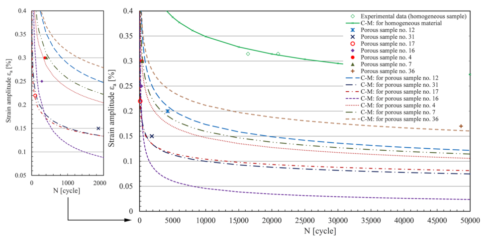
- In the final stage, the prediction of the service life is based on the case-wise adjusted Coffin–Manson curve of the porous material. Based on this curve, the fatigue life of the NB porous alloy can be estimated for a known load amplitude εB.
2.2. Application of Homogenised Approach
2.3. AlSi9Cu3 Alloy
2.4. Low-Cycle Fatigue Life
3. Numerical Simulations
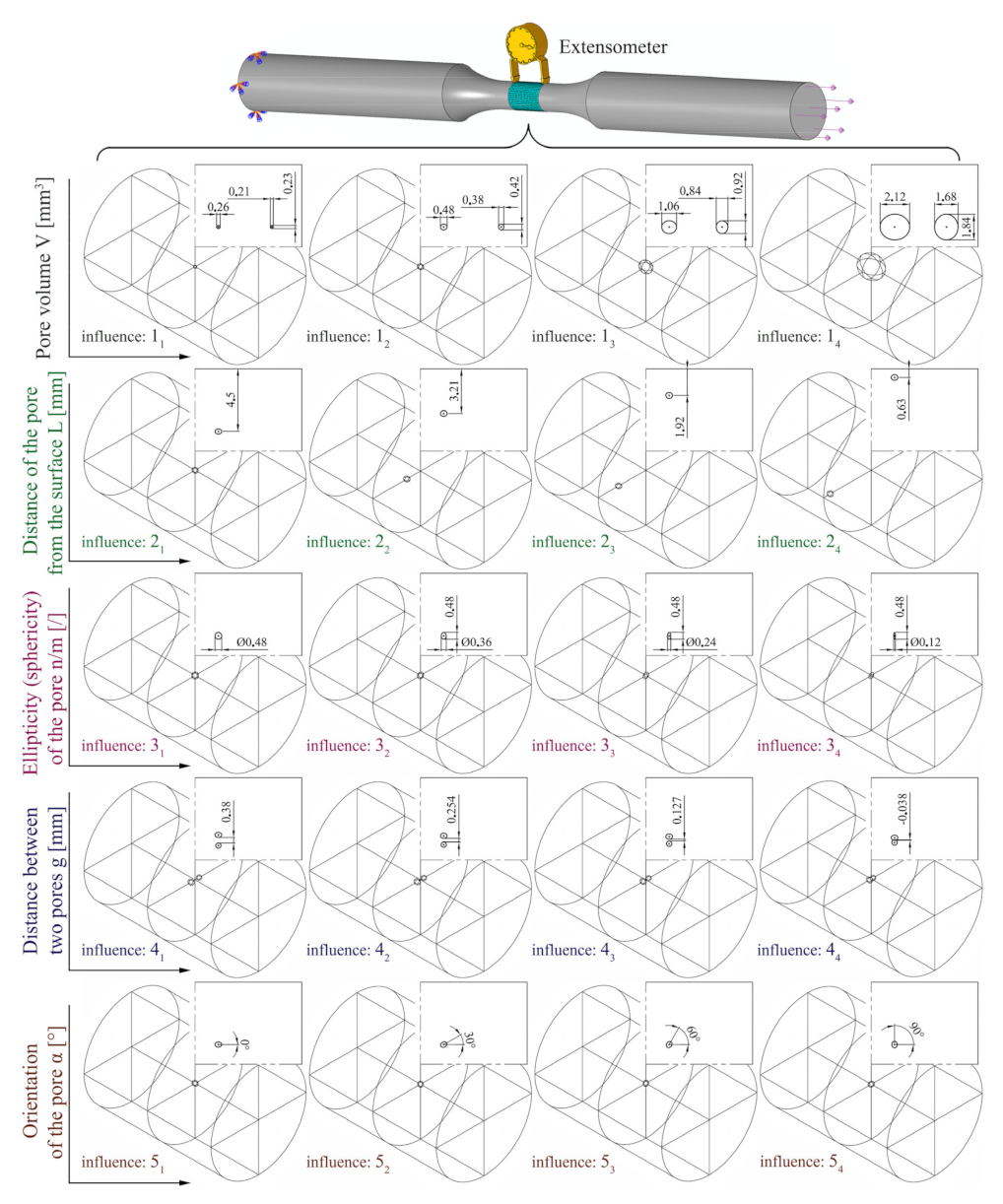
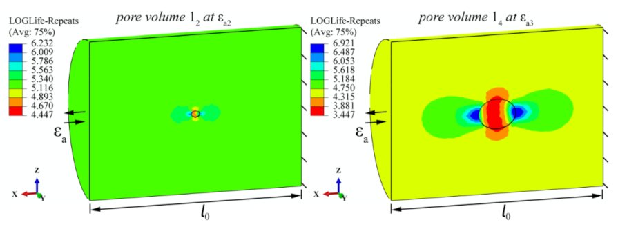
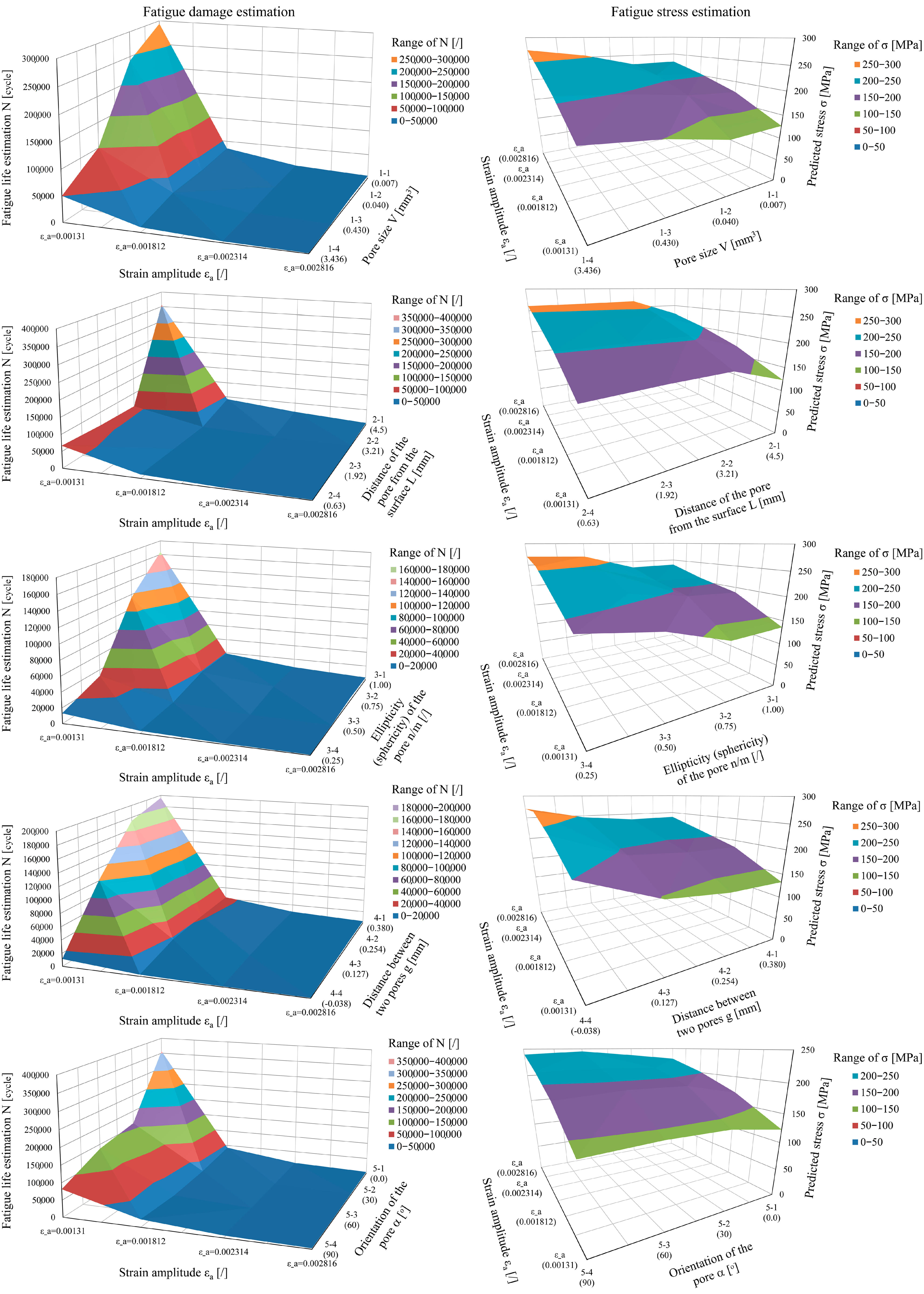
3.1. Separate Simulations for Each Geometric Parameter
- (11) V = Vmax/491 ≈ 0.007 mm3
- (12) V = Vaverage pore ≈ Vmax/86 ≈ 0.040 mm3
- (13) V = Vmax/8 ≈ 0.430 mm3
- (14) V = Vmax ≈ 3.436 mm3
- (21) L ≈ 10.8·dy(2) ≈ 4.5 mm (pore in the centre of the specimen)
- (22) L ≈ 7.7·dy(2) ≈ 3.21 mm
- (23) L ≈ 4.6·dy(2) ≈ 1.92 mm
- (24) L = 3/2·dy(2) ≈ 0.63 mm
- (31) n/m = 1 (sphere)
- (32) n/m = 0.75
- (33) n/m = 0.5
- (34) n/m = 0.25
- (41) g = dz(2) = 0.380 mm
- (42) g = 2/3·dz(2) ≈ 0.254 mm
- (43) g = 1/3·dz(2) ≈ 0.127 mm
- (44) g = −0.1·dz(2) ≈ −0.038 mm (overlapping of pores)
- (51) α = 0°
- (52) α = 30°
- (53) α = 60°
- (54) α = 90°
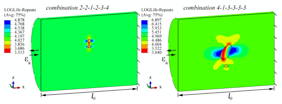
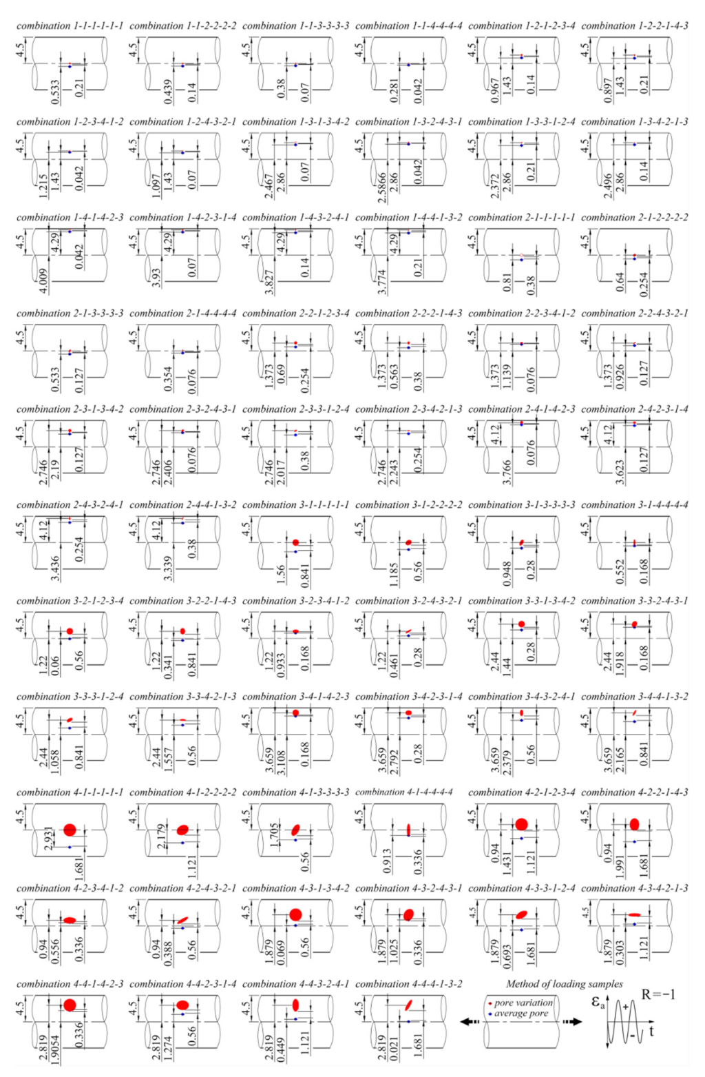
3.2. Simulations of Influences of Parameter Combinations on the Fatigue Life
3.3. Formulation of Equations to Calculate the Shift of the Synthetic εa–N Curve due to Porosity Effects
- (1)
- Pore size V (parameter x1 in the Taguchi array);
- (2)
- Distance of the pore from the surface of the specimen L (parameter x2 in the Taguchi array);
- (3)
- Pore ellipticity n/m (parameter x6 in the Taguchi array);
- (4)
- Distance between two pores g (parameter x10 in the Taguchi array);
- (5)
- Orientation of the pore α (parameter x14 in the Taguchi array).
4. Comparison of Theoretical and Experimental Results
5. Conclusions
- The method presented is an efficient and simple procedure for the estimation of the fatigue life, since the treatment of porosity starts from a homogeneous geometry, where fewer finite elements are used, and the influence of porosity is incorporated by a precise shift of the Coffin–Manson (C–M) εa–N durability curve.
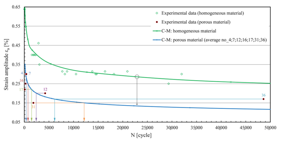
- As we have seen from experimental data, because of the large differences in the durability of differently porous samples, it is not reasonable to base the fatigue life calculation around one averagely shifted C–M curve because the predictions may be either too conservative or too optimistic. This brings us to the idea of individual treatment of a particular porous case.
- Modelling the synthetic durability C–M curve of a porous material based on regression calculations, its new terms σ′f and b, represents a significant advance in durability predictions according to the LCF theory since a simple preliminary analysis can give a reasonably good estimate of the fatigue life of a given porous specimen.
- The presented method allows the modelling of a synthetic C–M durability curve on two levels. By regression calculations of the coefficients si, bj, the basic course of the material durability curve is obtained first, which is then individually refined by entering the geometrical parameters x1–14 for a given analysed specimen. When studying porosity in AlSi9Cu3 alloy, it can be concluded from the simulations and regression analyses that this material is most sensitive to the geometric parameter of the orientation of the disc-shaped pores, defined by the regression coefficients s5 and b5. It is, therefore, important, when examining the porosity, to estimate as best as possible the angle α of the orientation of the dominant pores within the geometric influence x14.
- The prediction of the fatigue life is generally good on all samples analysed. The result is slightly more conservative only for sample no. 31, where the effect of the lamellarity of the structure around the central axis is more difficult to describe analytically via the ellipsoids used.
Author Contributions
Funding
Institutional Review Board Statement
Informed Consent Statement
Data Availability Statement
Acknowledgments
Conflicts of Interest
Nomenclature
| a,b,c | [mm] | Half-axes of ellipsoid |
| b | [-] | Fatigue strength exponent |
| b0,1,2,3,4,5 | [-] | Regression coefficients for estimating the Coffin–Manson exponent b |
| c | [-] | Fatigue ductility exponent |
| d | [mm] | Nominal diameter of the smallest half-axle of the ellipsoid |
| n/m | [-] | Sphericity ratio: quotient between the biggest and the smallest axle of the ellipsoid |
| n′ | [-] | Cyclic strain hardening exponent |
| p | [-] | Porosity |
| s0,1,2,3,4,5 | [-] | Regression coefficients for estimating the Coffin–Manson parameter σ′f |
| g | [mm] | Distance between two pores |
| l0 | [mm] | Gauge length (extensometer) |
| A | [mm2] | Cross-section |
| C–M | [-] | Coffin–Manson curve (equation) |
| D | [-] | Damage variable |
| E | [MPa] | Young’s modulus |
| K′ | [MPa] | Cyclic strain hardening coefficient |
| L | [mm] | The smallest distance between a pore boundary and a surface of the structure |
| Ln | [-] | Taguchi orthogonal array |
| N | [cycle] | Predicted fatigue life (cycles) |
| Nexp | [cycle] | Observed experimental fatigue life (cycles) |
| Nf | [cycle] | Number of cycles to failure |
| Ra | [μm] | Surface roughness |
| V | [mm3] | Pore volume |
| ε | [-] | Strain |
| εa | [-] | Strain amplitude |
| ε′f | [-] | Fatigue ductility coefficient |
| α | [°] | Pore direction: angle between the specimen longitudinal axis and the direction of the biggest pore half-axle |
| ν | [-] | Poisson’s ratio |
| ρ | [g/cm3] | Density |
| σ | [MPa] | Stress |
| σ′f | [MPa] | Fatigue strength coefficient |
| σm | [MPa] | Mean stress in the cycle |
| σmax | [MPa] | Maximum stress in the cycle |
| σu | [MPa] | Ultimate strength |
| σy | [MPa] | Yield strength |
| κt | [-] | Surface finish factor |
| Δl | [mm] | Length change |
| Δεn | [-] | Normal strain |
| Δγ | [-] | Shear strain |
References
- Anggraini, L. Sugeng Analysis of Porosity Defects in Aluminum as Part Handle Motor Vehicle Lever Processed by High-Pressure Die Casting. IOP Conf. Ser. Mater. Sci. Eng. 2018, 367, 012039. [Google Scholar] [CrossRef]
- Li, M.; Li, Y.; Zhou, H. Effects of Pouring Temperature on Microstructure and Mechanical Properties of the A356 Aluminum Alloy Diecastings. Mater. Res. 2020, 23, e20190676. [Google Scholar] [CrossRef]
- Murakami, Y.; Endo, M. Quantitative Evaluation of Fatigue Strength of Metals Containing Various Small Defects or Cracks. Eng. Fract. Mech. 1983, 17, 1–15. [Google Scholar] [CrossRef]
- Murakami, Y. Effects of Small Defects and Nonmetallic Inclusions on the Fatigue Strength of Metals. Key Eng. Mater. 1991, 51–52, 37–42. [Google Scholar] [CrossRef]
- Lee, H.W.; Basaran, C. A Review of Damage, Void Evolution, and Fatigue Life Prediction Models. Metals 2021, 11, 609. [Google Scholar] [CrossRef]
- Nečemer, B.; Vesenjak, M.; Glodež, S. Fatigue of Cellular Structures—A Review. SV-JME 2019, 65, 525–536. [Google Scholar] [CrossRef]
- Liu, A.F. Mechanics and Mechanisms of Fracture: An Introduction; ASM International: Materials Park, OH, USA, 2005; p. 500. [Google Scholar]
- Stephens, R.I.; Fatemi, A.; Stephens, R.R.; Fuchs, H.O. Metal Fatigue in Engineering, 2nd ed.; John Wiley & Sons: New York, NY, USA, 2001; p. 496. [Google Scholar]
- Spanos, P.D.; Sofi, A.; Wang, J.; Peng, B. A Method for Fatigue Analysis of Piping Systems on Topsides of FPSO Structures. J. Offshore Mech. Arct. Eng. 2006, 128, 162–168. [Google Scholar] [CrossRef]
- Al-Zubaidy, B.M.; AbidAli, A.K.; Athaib, N.H. Finite Element Analysis Of Porous Aluminium Aa3003 Alloy Under Compression And Bending Loading. Eur. J. Mol. Clin. Med. 2020, 7, 735–746. [Google Scholar]
- Tomažinčič, D.; Virk, Ž.; Kink, P.M.; Jerše, G.; Klemenc, J. Predicting the Fatigue Life of an AlSi9Cu3 Porous Alloy Using a Vector-Segmentation Technique for a Geometric Parameterisation of the Macro Pores. Metals 2020, 11, 72. [Google Scholar] [CrossRef]
- Kariyawasam, K.K.G.K.D.; Mallikarachchi, H.M.Y.C. Simulation of Low Cycle Fatigue with Abaqus/FEA. In Proceedings of the 3rd International Symposium on Advances in Civil and Environmental Engineering Practices for Sustainable Development (ACEPS—2015), Galle, Sri Lanka, 9 March 2015. [Google Scholar] [CrossRef]
- Upadhyaya, Y.S.; Sridhara, B.K. Fatigue Life Prediction: A Continuum Damage Mechanics and Fracture Mechanics Approach. Mater. Des. 2012, 35, 220–224. [Google Scholar] [CrossRef]
- Tomažinčič, D.; Borovinšek, M.; Ren, Z.; Klemenc, J. Improved Prediction of Low-Cycle Fatigue Life for High-Pressure Die-Cast Aluminium Alloy AlSi9Cu3 with Significant Porosity. Int. J. Fatigue 2021, 144, 106061. [Google Scholar] [CrossRef]
- Pawliczek, R.; Rozumek, D. Cyclic Tests of Smooth and Notched Specimens Subjected to Bending and Torsion Taking into Account the Effect of Mean Stress. Materials 2020, 13, 2141. [Google Scholar] [CrossRef] [PubMed]
- Yang, K.; Zhong, B.; Huang, Q.; He, C.; Huang, Z.-Y.; Wang, Q.; Liu, Y.-J. Stress Ratio and Notch Effects on the Very High Cycle Fatigue Properties of a Near-Alpha Titanium Alloy. Materials 2018, 11, 1778. [Google Scholar] [CrossRef] [PubMed] [Green Version]
- Nečemer, B.; Glodež, S.; Novak, N.; Kramberger, J. Numerical Modelling of a Chiral Auxetic Cellular Structure under Multiaxial Loading Conditions. Theor. Appl. Fract. Mech. 2020, 107, 102514. [Google Scholar] [CrossRef]
- Klemenc, J.; Nagode, M. Design of Step-stress Accelerated Life Tests for Estimating the Fatigue Reliability of Structural Components Based on a Finite-element Approach. Fatigue Fract. Eng. Mater. Struct. 2021, 44, 1562–1582. [Google Scholar] [CrossRef]
- Tomazincic, D.; Sedlacek, M.; Podgornik, B.; Klemenc, J. Influence of different micro-imprints to fatigue life of components. Mater. Perform. Charact. 2017, 6, 79–95. [Google Scholar] [CrossRef]
- Ricotta, M. Simple Expressions to Estimate the Manson–Coffin Curves of Ductile Cast Irons. Int. J. Fatigue 2015, 78, 38–45. [Google Scholar] [CrossRef]
- Peng, H.; Fan, J.; Zhang, X.; Chen, J.; Li, Z.; Jiang, D.; Liu, C. Computed Tomography Analysis on Cyclic Fatigue and Damage Properties of Rock Salt under Gas Pressure. Int. J. Fatigue 2020, 134, 105523. [Google Scholar] [CrossRef]
- Aguilar, C.; Arancibia, M.; Alfonso, I.; Sancy, M.; Tello, K.; Salinas, V.; De Las Cuevas, F. Influence of Porosity on the Elastic Modulus of Ti-Zr-Ta-Nb Foams with a Low Nb Content. Metals 2019, 9, 176. [Google Scholar] [CrossRef] [Green Version]
- Bergant, M.; Werner, T.; Madia, M.; Yawny, A.; Zerbst, U. Short Crack Propagation Analysis and Fatigue Strength Assessment of Additively Manufactured Materials: An Application to AISI 316L. Int. J. Fatigue 2021, 151, 106396. [Google Scholar] [CrossRef]
- Klemenc, J.; Fajdiga, M. Joint estimation of E–N curves and their scatter using evolutionary algorithms. Int. J. Fatigue 2013, 56, 42–53. [Google Scholar] [CrossRef]
- DNVGL-ST-0361. Machinery for Wind Turbines; DNV Holding AS: Høvik, Norway, 2016; p. 61. [Google Scholar]
- Susmel, L. Multiaxial Notch Fatigue: From Nominal to Local Stress/Strain Quantities; Woodhead Publishing Limited and CRC Press LLC: New York, NY, USA, 2009; p. 727. [Google Scholar]
- Murakami, Y.; Endo, T. Effects of Small Defects on Fatigue Strength of Metals. Int. J. Fatigue 1980, 2, 23–30. [Google Scholar] [CrossRef]
- Bižal, A.; Klemenc, J.; Fajdiga, M. Modelling the Fatigue Life Reduction of an AlSi9Cu3 Alloy Caused by Macro-Porosity. Eng. Comput. 2015, 31, 259–269. [Google Scholar] [CrossRef]
- Morgan, K.E. Standard Practice for Strain-Controlled Fatigue Testing; ASTM E606–92(2004)e1; ASTM International: West Conshohocken, PA, USA, 2004; p. 15. [Google Scholar]
- Li, Y.; Shterenlikht, A.; Pavier, M.; Coules, H. Fatigue of Thin Periodic Triangular Lattice Plates. MATEC Web Conf. 2019, 300, 03002. [Google Scholar] [CrossRef] [Green Version]
- Cui, T.; Mukherjee, S.; Sudeep, P.M.; Colas, G.; Najafi, F.; Tam, J.; Ajayan, P.M.; Singh, C.V.; Sun, Y.; Filleter, T. Fatigue of Graphene. Nat. Mater. 2020, 19, 405–411. [Google Scholar] [CrossRef]
- Szalva, P.; Orbulov, I.N. Effects of Artificial and Natural Defects on Fatigue Strength of a Cast Aluminum Alloy. Fatigue Fract. Eng. Mater. Struct. 2021, 44, 3214–3218. [Google Scholar] [CrossRef]
- Bogdanoff, T.; Lattanzi, L.; Merlin, M.; Ghassemali, E.; Jarfors, A.E.W.; Seifeddine, S. The Complex Interaction between Microstructural Features and Crack Evolution during Cyclic Testing in Heat-Treated Al–Si–Mg–Cu Cast Alloys. Mater. Sci. Eng. A 2021, 825, 141930. [Google Scholar] [CrossRef]
- Brown, M.W.; Miller, K.J. A theory for fatigue failure under multiaxial stress–strain conditions. Proc. Inst. Mech. Eng. 1973, 187, 745–755. [Google Scholar] [CrossRef]
- Corp, D.S.S. SIMULIA Fe-Safe. User Guide, 1st ed.; Dassault Systemes: Vélizy-Villacoublay, France, 2019; p. 445. [Google Scholar]
- Parks, J.M. On Stochastic Optimization: Taguchi Methods™ demystified; Its limitations and fallacy clarified. Probabilistic Eng. Mech. 2001, 16, 87–101. [Google Scholar] [CrossRef]
- Ross, P.J. Taguchi Techniques for Quality Engineering, 2nd ed.; McGraw Hill Professional: New York, NY, USA, 1996; p. 329. [Google Scholar]
- Kacker, R.N.; Lagergren, E.S.; Filliben, J.J. Taguchi’s Orthogonal Arrays Are Classical Designs of Experiments. J. Res. Natl. Inst. Stand. Technol. 1991, 96, 577. [Google Scholar] [CrossRef]
- Ma, Y.; Wang, Q.; Guo, Z.; Wang, G.; Wang, L.; Zhang, J. Static and Fatigue Behavior Investigation of Artificial Notched Steel Reinforcement. Materials 2017, 10, 532. [Google Scholar] [CrossRef] [PubMed] [Green Version]
- Milella, P.P. Notch Effect. In Fatigue and Corrosion in Metals; Springer: Milano, Italy, 2013; pp. 365–403. [Google Scholar] [CrossRef]


| Sp. No. | Strain εa [%] | Number of Cycles Reached Nexp | Volume of the Critical Pore ‡ V [mm3] | Distance of the Pore from the Surface L [mm] | Ellipticity of the Poren/m [/] | Distance between Two Pores g [mm] | Orientation of the Pore α [°] | C–M of the Porous Structure | |
|---|---|---|---|---|---|---|---|---|---|
| x1 | x2 | x6 | x10 | x14 | σ′f | b | |||
| 12 | 0.2 * (0.19 **) | 4243 | 2.7 | 2.3 | 0.95 | 0.25 | 1 | 1063 | −0.22 |
| 31 | 0.15 * (0.13 **) | 1853 | 0.17 | 4.5 | 0.35 | 0.5 | 12 | 411 | −0.18 |
| 36 | 0.17 * (0.16 **) | 48,619 | 0.11 | 2.2 | 0.85 | 1 | 2 | 801 | −0.172 |
| 17 | 0.22 * (0.21 **) | 98 | 1.3 | 4 | 0.1 | –0.1 | 12 | 331 | −0.154 |
| 16 | 0.25 * (0.25 **) | 282 | 16.7 | 2.5 | 0.9 | –0.2 | 4 | 1790 | −0.408 |
| 4 | 0.3 * (0.28 **) | 370 | 0.83 | 3.6 | 0.95 | 0.2 | 6 | 772 | −0.205 |
| 7 | 0.3 * (0.28 **) | 415 | 1.3 | 3.8 | 0.9 | 0.2 | 4 | 851 | −0.206 |
| (1) Pore Size (Volume) V | ||||||||
|---|---|---|---|---|---|---|---|---|
| / | (6) Strain Level εa | |||||||
| εa1 = 0.00131 | εa2 = 0.001812 | εa3 = 0.002314 | εa4 = 0.002816 | |||||
| Stress σ [MPa] | Cycles N [Cycle] | Stress σ [MPa] | Cycles N [Cycle] | Stress σ [MPa] | Cycles N [Cycle] | Stress σ [MPa] | Cycles N [Cycle] | |
| 11 | 127 | 5.468 * (293,764) | 175 | 4.536 * (34,356) | 204 | 4.061 * (11,508) | 227 | 3.689 * (4887) |
| 12 | 122 | 5.384 * (242,103) | 181 | 4.447 * (27,990) | 209 | 3.966 * (9247) | 225 | 3.712 * (5152) |
| 13 | 149 | 5.004 * (100,925) | 197 | 4.433 * (27,102) | 226 | 3.689 * (4887) | 254 | 3.261 * (1824) |
| 14 | 165 | 4.702 * (50,350) | 208 | 3.987 * (9705) | 241 | 3.447 * (2799) | 271 | 2.996 * (991) |
| (2) Distance of the pore from the surface L | ||||||||
| 21 | 123 | 5.552 * (356,451) | 170 | 4.621 * (41,783) | 202 | 4.294 * (19,679) | 226 | 3.698 * (4989) |
| 22 | 162 | 4.751 * (56,364) | 206 | 4.012 * (10,280) | 239 | 3.486 * (3062) | 266 | 3.075 * (1189) |
| 23 | 161 | 4.771 * (59,020) | 204 | 4.039 * (10,940) | 236 | 3.506 * (3206) | 263 | 3.082 * (1208) |
| 24 | 157 | 4.825 * (66,834) | 202 | 4.053 * (11,298) | 233 | 3.548 * (3532) | 261 | 3.125 * (1334) |
| (3) Ellipticity of the pore n/m | ||||||||
| 31 | 136 | 5.214 * (163,682) | 188 | 4.275 * (18,836) | 209 | 3.911 * (8147) | 236 | 3.495 * (3126) |
| 32 | 131 | 5.064 * (115,878) | 192 | 4.276 * (18,880) | 209 | 3.953 * (8974) | 233 | 3.577 * (3776) |
| 33 | 171 | 4.502 * (31,769) | 210 | 3.845 * (6998) | 242 | 3.331 * (2143) | 267 | 2.973 * (940) |
| 34 | 190 | 4.120 * (13,183) | 223 | 3.535 * (3428) | 256 | 3.070 * (1175) | 270 | 2.842 * (695) |
| (4) Distance between two pores g | ||||||||
| 41 | 133 | 5.291 * (195,434) | 184 | 4.356 * (22,699) | 211 | 3.888 * (7727) | 237 | 3.473 * (2972) |
| 42 | 134 | 5.241 * (174,181) | 185 | 4.323 * (21,038) | 209 | 3.917 * (8260) | 235 | 3.501 * (3170) |
| 43 | 147 | 5.005 * (101,158) | 193 | 4.245 * (17,579) | 219 | 3.791 * (6180) | 246 | 3.373 * (2360) |
| 44 | 200 | 4.054 * (11,324) | 241 | 3.402 * (2523) | 271 | 2.953 * (897) | 271 | 2.842 * (695) |
| (5) Orientation of the pore α | ||||||||
| 51 | 123 | 5.552 * (356,451) | 170 | 4.621 * (41,783) | 202 | 4.072 * (11,803) | 226 | 3.698 * (4989) |
| 52 | 139 | 5.207 * (161,065) | 190 | 4.406 * (25,468) | 214 | 3.945 * (8810) | 236 | 3.560 * (3631) |
| 53 | 141 | 5.136 * (136,773) | 191 | 4.247 * (17,660) | 216 | 3.820 * (6607) | 245 | 3.374 * (2366) |
| 54 | 137 | 4.911 * (81,470) | 184 | 4.356 * (22,699) | 215 | 3.826 * (6699) | 240 | 3.431 * (2698) |
| Pore Volume V | Taguchi Combinations | Stress σ [MPa] | Cycles N [Cycle] | Pore Volume V | Taguchi Combination | Stress σ [MPa] | Cycles N [Cycle] | ||||||||||
|---|---|---|---|---|---|---|---|---|---|---|---|---|---|---|---|---|---|
| x1 | x2 | x6 | x10 | x14 | x18 | x1 | x2 | x6 | x10 | x14 | x18 | ||||||
| 11 | 1-1-1-1-1-1 | 124 | 5.113 * (129,718) | 13 | 3-1-1-1-1-1 | 147 | 5.000 * (100,000) | ||||||||||
| 1-1-2-2-2-2 | 188 | 4.302 * (20,045) | 3-1-2-2-2-2 | 206 | 3.986 * (9683) | ||||||||||||
| 1-1-3-3-3-3 | 268 | 3.001 * (1002) | 3-1-3-3-3-3 | 252 | 3.192 * (1556) | ||||||||||||
| 1-1-4-4-4-4 | 271 | 2.713 * (516) | 3-1-4-4-4-4 | 271 | 2.555 * (359) | ||||||||||||
| 1-2-1-2-3-4 | 239 | 3.479 * (3013) | 3-2-1-2-3-4 | 258 | 3.187 * (1538) | ||||||||||||
| 1-2-2-1-4-3 | 208 | 3.958 * (908) | 3-2-2-1-4-3 | 237 | 3.487 * (3069) | ||||||||||||
| 1-2-3-4-1-2 | 217 | 3.432 * (2704) | 3-2-3-4-1-2 | 214 | 3.883 * (7638) | ||||||||||||
| 1-2-4-3-2-1 | 178 | 4.367 * (23,281) | 3-2-4-3-2-1 | 188 | 4.047 * (11,143) | ||||||||||||
| 1-3-1-3-4-2 | 203 | 4.074 * (11,858) | 3-3-1-3-4-2 | 205 | 4.033 * (10,789) | ||||||||||||
| 1-3-2-4-3-1 | 204 | 3.779 * (6012) | 3-3-2-4-3-1 | 188 | 3.996 * (9908) | ||||||||||||
| 1-3-3-1-2-4 | 254 | 3.252 * (1786) | 3-3-3-1-2-4 | 260 | 3.161 * (1449) | ||||||||||||
| 1-3-4-2-1-3 | 207 | 4.010 * (10,233) | 3-3-4-2-1-3 | 206 | 4.032 * (10,765) | ||||||||||||
| 1-4-1-4-2-3 | 252 | 3.214 * (1637) | 3-4-1-4-2-3 | 259 | 3.173 * (1489) | ||||||||||||
| 1-4-2-3-1-4 | 258 | 3.210 * (1622) | 3-4-2-3-1-4 | 270 | 3.000 * (1000) | ||||||||||||
| 1-4-3-2-4-1 | 186 | 4.288 * (19,409) | 3-4-3-2-4-1 | 201 | 4.000 * (10,000) | ||||||||||||
| 1-4-4-1-3-2 | 240 | 3.342 * (2198) | 3-4-4-1-3-2 | 265 | 2.928 * (847) | ||||||||||||
| 12 | 2-1-1-1-1-1 | 128 | 5.269 * (185,780) | 14 | 4-1-1-1-1-1 | 181 | 4.422 * (26,424) | ||||||||||
| 2-1-2-2-2-2 | 189 | 4.269 * (18,578) | 4-1-2-2-2-2 | 217 | 3.823 * (6653) | ||||||||||||
| 2-1-3-3-3-3 | 240 | 3.395 * (2483) | 4-1-3-3-3-3 | 264 | 3.040 * (1096) | ||||||||||||
| 2-1-4-4-4-4 | 271 | 2.812 * (649) | 4-1-4-4-4-4 | 271 | 2.558 * (361) | ||||||||||||
| 2-2-1-2-3-4 | 236 | 3.515 * (3273) | 4-2-1-2-3-4 | 271 | 2.926 * (843) | ||||||||||||
| 2-2-2-1-4-3 | 209 | 3.942 * (8750) | 4-2-2-1-4-3 | 270 | 2.959 * (910) | ||||||||||||
| 2-2-3-4-1-2 | 204 | 4.034 * (10,814) | 4-2-3-4-1-2 | 203 | 4.052 * (11,272) | ||||||||||||
| 2-2-4-3-2-1 | 127 | 5.215 * (16,406) | 4-2-4-3-2-1 | 194 | 3.896 * (7870) | ||||||||||||
| 2-3-1-3-4-2 | 192 | 4.272 * (18,707) | 4-3-1-3-4-2 | 219 | 3.775 * (5957) | ||||||||||||
| 2-3-2-4-3-1 | 167 | 3.741 * (5508) | 4-3-2-4-3-1 | 187 | 4.318 * (20,800) | ||||||||||||
| 2-3-3-1-2-4 | 250 | 3.301 * (2000) | 4-3-3-1-2-4 | 270 | 2.996 * (991) | ||||||||||||
| 2-3-4-2-1-3 | 210 | 3.926 * (8433) | 4-3-4-2-1-3 | 208 | 3.985 * (9661) | ||||||||||||
| 2-4-1-4-2-3 | 264 | 2.990 * (977) | 4-4-1-4-2-3 | 266 | 3.079 * (1199) | ||||||||||||
| 2-4-2-3-1-4 | 252 | 3.306 * (2023) | 4-4-2-3-1-4 | 271 | 2.978 * (951) | ||||||||||||
| 2-4-3-2-4-1 | 175 | 4.489 * (30,832) | 4-4-3-2-4-1 | 192 | 4.024 * (10,568) | ||||||||||||
| 2-4-4-1-3-2 | 243 | 3.308 * (2032) | 4-4-4-1-3-2 | 271 | 2.796 * (625) | ||||||||||||
| Combinations from Taguchi Array | Brown–Miller–Morrow (B–M–M) | Smith–Watson–Topper (S–W–T) | Comment of the Results |
|---|---|---|---|
| 2-2-1-2-3-4 | 3.515 * (3273) | 3.583 * (3828) | When considering pores of the same size with mutual distances g < 0.38 mm, the B–M–M criterion gives slightly more conservative results. The reason may be the additional inclusion of the shear stress in the B–M–M criterion, which has an additional impact on the interaction between the proximal pores. |
| 4-1-3-3-3-3 | 3.040 * (1096) | 3.086 * (1219) | If there is a combination of the dominant pores in the middle of the sample and the distance between the pores g > 0.38 mm, the criteria B–M–M and S–W–T are comparable, with minimal differences in the prediction of the duration. In this case too, the B–M–M criterion is somewhat more conservative. |
Publisher’s Note: MDPI stays neutral with regard to jurisdictional claims in published maps and institutional affiliations. |
© 2022 by the authors. Licensee MDPI, Basel, Switzerland. This article is an open access article distributed under the terms and conditions of the Creative Commons Attribution (CC BY) license (https://creativecommons.org/licenses/by/4.0/).
Share and Cite
Tomažinčič, D.; Klemenc, J. Estimate of Coffin–Manson Curve Shift for the Porous Alloy AlSi9Cu3 Based on Numerical Simulations of a Porous Material Carried Out by Using the Taguchi Array. Materials 2022, 15, 2269. https://doi.org/10.3390/ma15062269
Tomažinčič D, Klemenc J. Estimate of Coffin–Manson Curve Shift for the Porous Alloy AlSi9Cu3 Based on Numerical Simulations of a Porous Material Carried Out by Using the Taguchi Array. Materials. 2022; 15(6):2269. https://doi.org/10.3390/ma15062269
Chicago/Turabian StyleTomažinčič, Dejan, and Jernej Klemenc. 2022. "Estimate of Coffin–Manson Curve Shift for the Porous Alloy AlSi9Cu3 Based on Numerical Simulations of a Porous Material Carried Out by Using the Taguchi Array" Materials 15, no. 6: 2269. https://doi.org/10.3390/ma15062269