

An HGA-LSTM-Based Intelligent Model for Ore Pulp Density in the Hydrometallurgical Process

Abstract
:1. Introduction
- We introduced an intelligent model to resolve the difficulty encountered in measuring the feed density in the thickener through online real-time detection in hydrometallurgy.
- A novel intelligent modeling method combining SQP, GA, and LSTM was developed to address the nonlinear and dynamic background. The HGA algorithm was used to optimize the hyperparameters of the LSTM.
- From the perspective of actual cases, the results show that the method fulfills the measurement requirements in the factory.
2. Methodology
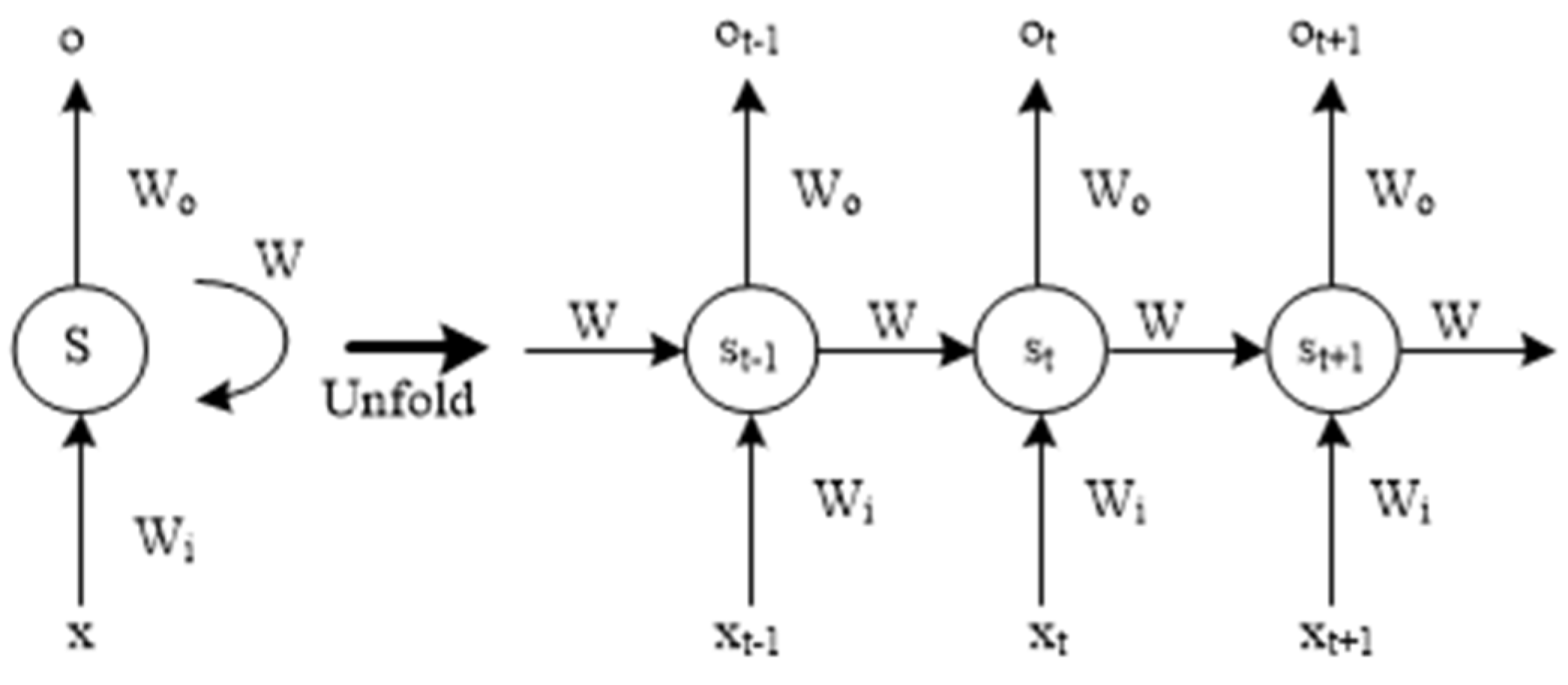
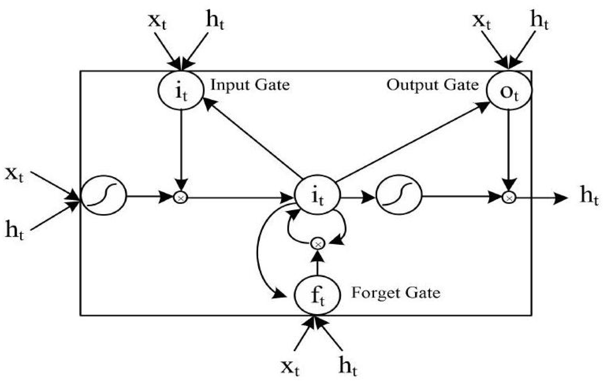
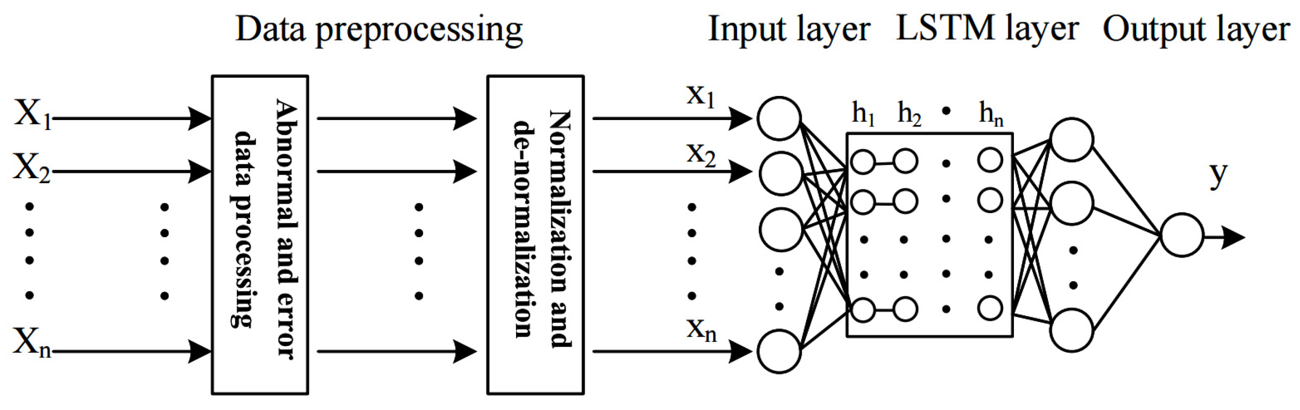
2.1. LSTM Network
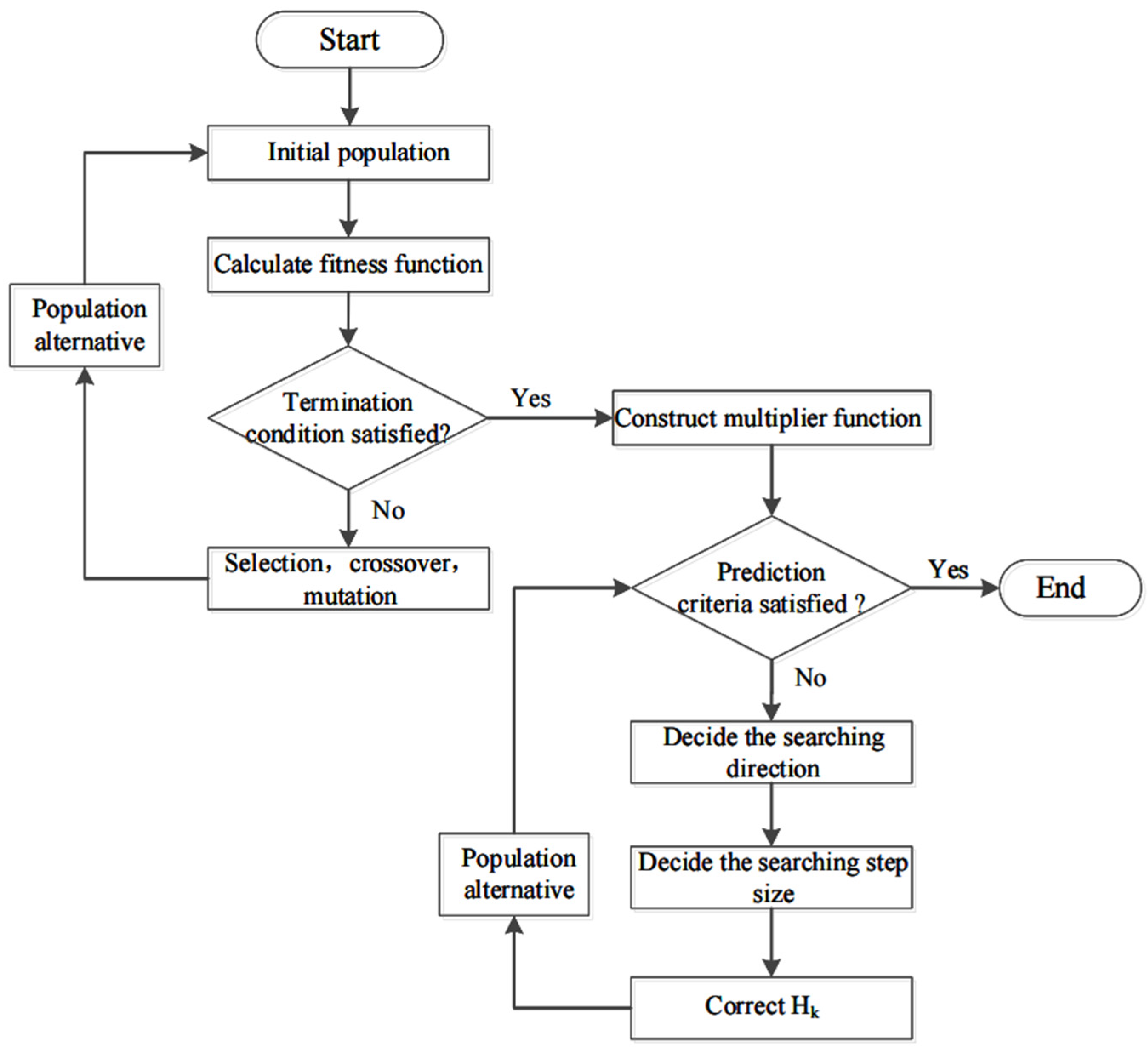
2.2. Hybrid Genetic Algorithm
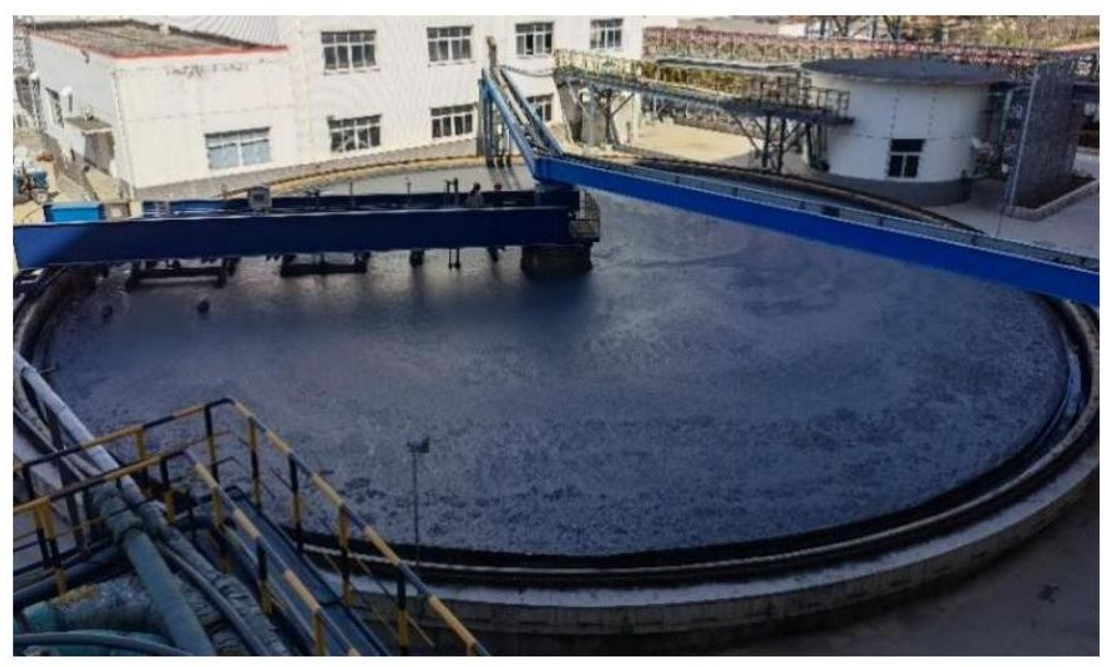
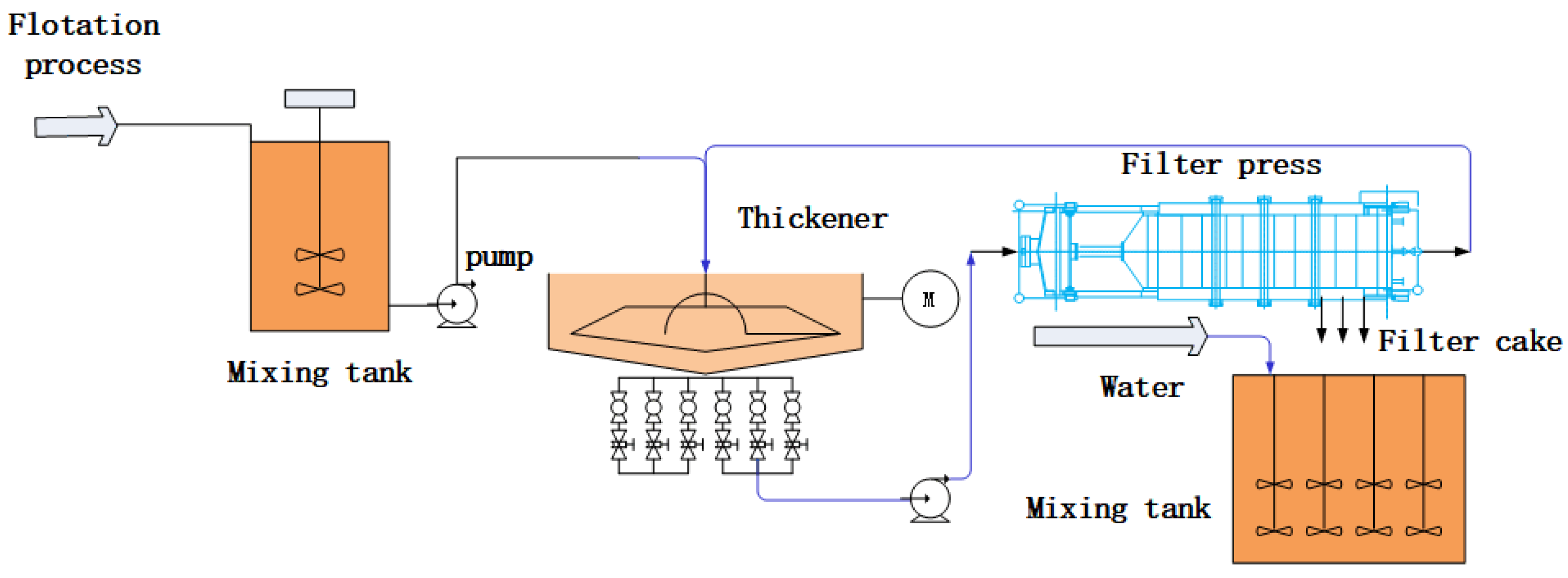
3. Process Description
4. Intelligent Model Based on HGA-LSTM
4.1. Data Preprocessing
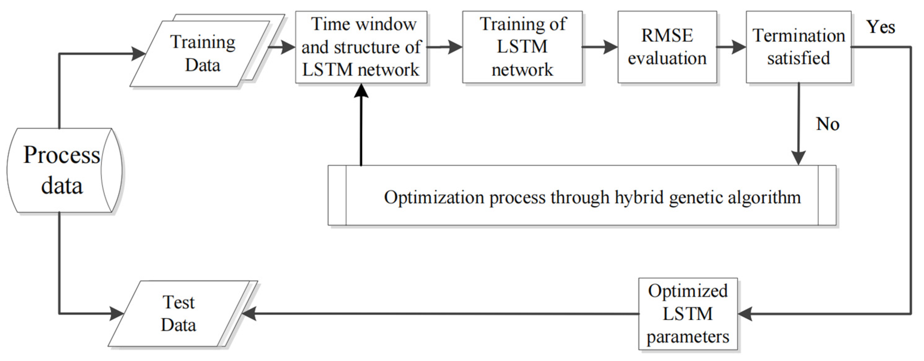
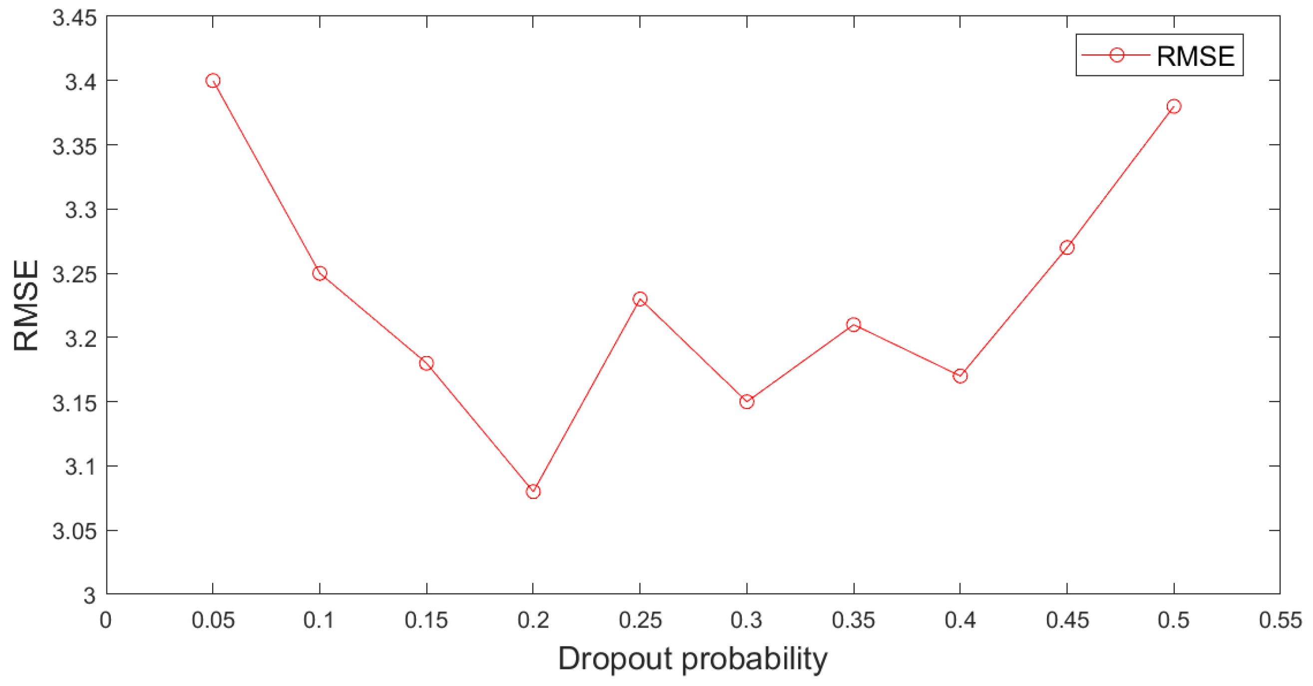
4.2. LSTM Network Training and Hyperparameter Optimization
| Algorithm 1 HGA–LSTM steps |
| 1. Divide the raw data into a test set and training set; 2. Use the test data to evaluate the LSTM; 3. Set GA parameters, and initialize population p randomly; 4. Select the RMSE of LSTM in the testing set as the fitness function of GA; 5. While the prediction criteria are not satisfied: (a) Select befitting parents from the population; (b) Generate a new population through crossover and mutation of chromosomes; (c) Consider the individual chromosome that includes the time window, hidden layers, and number of hidden units per hidden layer into the LSTM to evaluate the fitness of the new population; End |
| 6. Set the five fast convergence values of output GA as the initial values of SQP, fit a modified fitness function, and set ; |
| 7. Calculate the quasi-Newton approximation matrix of the language function using the BFGS method at ; |
| 8. Calculate the search direction , and select the appropriate step length parameter ; |
| If satisfactory, stop; else set , , and return to step 7; |
| 9. Discrete and output the optimal solution of the SQP, which is the hyperparameter of the LSTM network; |
| 10. Use the well-trained LSTM network for soft sensor modeling, and evaluate the predicted results. |
5. Experimental Results
5.1. Dataset Description
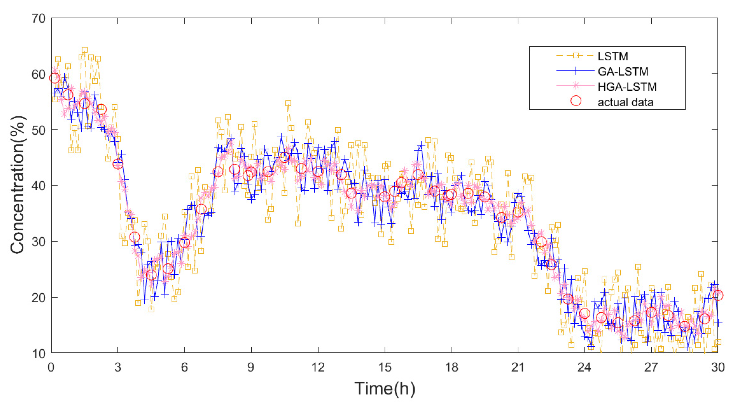
5.2. Results Analysis
6. Conclusions
Author Contributions
Funding
Conflicts of Interest
References
- La Brooy, S.; Linge, H.; Walker, G. Review of gold extraction from ores. Miner. Eng. 1994, 7, 1213–1241. [Google Scholar] [CrossRef]
- Yan, H.; Wang, F.; He, D.; Wang, Q. An operational adjustment framework for a complex industrial process based on hybrid Bayesian network. IEEE Trans. Autom. Sci. Eng. 2020, 17, 1699–1710. [Google Scholar] [CrossRef]
- Tan, C.K.; Bao, J.; Bickert, G. A study on model predictive control in paste thickeners with rake torque constraint. Miner. Eng. 2017, 105, 52–62. [Google Scholar] [CrossRef]
- Jia, R.; Zhang, B.; He, D.; Mao, Z.; Chu, F. Data-driven-based self-healing control of abnormal feeding conditions in thickening–dewatering process. Miner. Eng. 2020, 146, 106141. [Google Scholar] [CrossRef]
- Jiang, Y.; Yin, S.; Dong, J.; Kaynak, O. A review on soft sensors for monitoring, control, and optimization of industrial processes. IEEE Sens. J. 2020, 21, 12868–12881. [Google Scholar] [CrossRef]
- Kim, B.; Lee, D.E.; Preethaa, K.S.; Hu, G.; Natarajan, Y.; Kwok, K. Predicting wind flow around buildings using deep learning. J. Wind Eng. Ind. Aerodyn. 2021, 219, 104820. [Google Scholar] [CrossRef]
- Kim, B.; Yuvaraj, N.; Sri Preethaa, K.R.; Hu, G.; Lee, D.E. Wind-Induced Pressure Prediction on Tall Buildings Using Generative Adversarial Imputation Network. Sensors 2021, 21, 2515. [Google Scholar] [CrossRef]
- Dai, J.; Chen, N.; Yuan, X.; Gui, W.; Luo, L. Temperature prediction for roller kiln based on hybrid first-principle model and data-driven MW-DLWKPCR model. ISA Trans. 2020, 98, 403–417. [Google Scholar] [CrossRef]
- Kim, B.; Yuvaraj, N.; Sri Preethaa, K.R.; Arun Pandian, R. Surface crack detection using deep learning with shallow CNN architecture for enhanced computation. Neural Comput. Appl. 2021, 33, 9289–9305. [Google Scholar] [CrossRef]
- Kadlec, P.; Gabrys, B.; Strandt, S. Data-driven soft sensors in the process industry. Comput. Chem. Eng. 2009, 33, 795–814. [Google Scholar] [CrossRef]
- Kaneko, H.; Funatsu, K. Application of online support vector regression for soft sensors. AIChE J. 2014, 60, 600–612. [Google Scholar] [CrossRef]
- Yang, K.; Jin, H.; Chen, X.; Dai, J.; Wang, L.; Zhang, D. Soft sensor development for online quality prediction of industrial batch rubber mixing process using ensemble just-in-time Gaussian process regression models. Chemom. Intell. Lab. Syst. 2016, 155, 170–182. [Google Scholar] [CrossRef]
- Pisa, I.; Santín, I.; Vicario, J.L.; Morell, A.; Vilanova, R. ANN-based soft sensor to predict effluent violations in wastewater treatment plants. Sensors 2019, 19, 1280. [Google Scholar] [CrossRef] [PubMed] [Green Version]
- Popli, K.; Afacan, A.; Liu, Q.; Prasad, V. Development of online soft sensors and dynamic fundamental model-based process monitoring for complex sulfide ore flotation. Miner. Eng. 2018, 124, 10–27. [Google Scholar] [CrossRef]
- Mou, L.; Ghamisi, P.; Zhu, X.X. Deep recurrent neural networks for hyperspectral image classification. IEEE Trans. Geosci. Remote Sens. 2017, 55, 3639–3655. [Google Scholar] [CrossRef] [Green Version]
- Yan, H.; Wang, F.; He, D.; Zhao, L.; Wang, Q. Bayesian network-based modeling and operational adjustment of plantwide flotation industrial process. Ind. Eng. Chem. Res. 2020, 59, 2025–2035. [Google Scholar] [CrossRef]
- Zhou, Q.; Ooka, R. Comparison of different deep neural network architectures for isothermal indoor airflow prediction. In Building Simulation; Springer: Berlin/Heidelberg, Germany, 2020; Volume 13, pp. 1409–1423. [Google Scholar]
- Yuan, X.; Qi, S.; Wang, Y. Stacked enhanced auto-encoder for data-driven soft sensing of quality variable. IEEE Trans. Instrum. Meas. 2020, 69, 7953–7961. [Google Scholar] [CrossRef]
- Yan, H.; Wang, F.; Yan, G.; He, D. Hybrid approach integrating case-based reasoning and Bayesian network for operational adjustment in industrial flotation process. J. Process Control 2021, 103, 34–47. [Google Scholar] [CrossRef]
- Sherstinsky, A. Fundamentals of recurrent neural network (RNN) and long short-term memory (LSTM) network. Phys. D Nonlinear Phenom. 2020, 404, 132306. [Google Scholar] [CrossRef] [Green Version]
- Hochreiter, S.; Schmidhuber, J. Long short-term memory. Neural Comput. 1997, 9, 1735–1780. [Google Scholar] [CrossRef]
- Zhang, H.; Tang, Z.; Xie, Y.; Gao, X.; Chen, Q.; Gui, W. Long short-term memory-based grade monitoring in froth flotation using a froth video sequence. Miner. Eng. 2021, 160, 106677. [Google Scholar] [CrossRef]
- Pan, H.; Su, T.; Huang, X.; Wang, Z. LSTM-based soft sensor design for oxygen content of flue gas in coal-fired power plant. Trans. Inst. Meas. Control 2021, 43, 78–87. [Google Scholar] [CrossRef]
- Ke, W.; Huang, D.; Yang, F.; Jiang, Y. Soft sensor development and applications based on LSTM in deep neural networks. In Proceedings of the 2017 IEEE Symposium Series on Computational Intelligence (SSCI). IEEE, Honolulu, HI, USA, 27 November–1 December 2017; pp. 1–6. [Google Scholar]
- Bouktif, S.; Fiaz, A.; Ouni, A.; Serhani, M.A. Optimal deep learning lstm model for electric load forecasting using feature selection and genetic algorithm: Comparison with machine learning approaches. Energies 2018, 11, 1636. [Google Scholar] [CrossRef] [Green Version]
- Chung, H.; Shin, K.S. Genetic algorithm-optimized long short-term memory network for stock market prediction. Sustainability 2018, 10, 3765. [Google Scholar] [CrossRef] [Green Version]
- Alshwaheen, T.I.; Hau, Y.W.; Ass’Ad, N.; Abualsamen, M.M. A novel and reliable framework of patient deterioration prediction in intensive care unit based on long short-term memory-recurrent neural network. IEEE Access 2020, 9, 3894–3918. [Google Scholar] [CrossRef]
- Jahed Armaghani, D.; Hasanipanah, M.; Mahdiyar, A.; Abd Majid, M.Z.; Bakhshandeh Amnieh, H.; Tahir, M. Airblast prediction through a hybrid genetic algorithm-ANN model. Neural Comput. Appl. 2018, 29, 619–629. [Google Scholar] [CrossRef]
- Zhang, Y.; Li, J.; Fan, X.; Liu, J.; Zhang, H. Moisture prediction of transformer oil-immersed polymer insulation by applying a support vector machine combined with a genetic algorithm. Polymers 2020, 12, 1579. [Google Scholar] [CrossRef]
- Mandic, D.P.; Chambers, J.A. Exploiting inherent relationships in RNN architectures. Neural Netw. 1999, 12, 1341–1345. [Google Scholar] [CrossRef]
- Felix, A.G.; Jürgen, S.; Fred, C. Learning to forget: Continual prediction with LSTM. Neural Comput. 2000, 12, 2451–2471. [Google Scholar]
- Li, Y.C.; Zhao, L.N.; Zhou, S.J. Review of Genetic Algorithm. Adv. Mater. Res. 2011, 179–180, 365–367. [Google Scholar] [CrossRef]
- Fletcher, R.; Leyffer, S.; Ralph, D.; Scholtes, S. Local convergence of SQP methods for mathematical programs with equilibrium constraints. SIAM J. Optim. 2006, 17, 259–286. [Google Scholar] [CrossRef]
- Mansoornejad, B.; Mostoufi, N.; Jalali-Farahani, F. A hybrid GA–SQP optimization technique for determination of kinetic parameters of hydrogenation reactions. Comput. Chem. Eng. 2008, 32, 1447–1455. [Google Scholar] [CrossRef]
- Li, K.; Wang, F.; He, D.; Zhang, S. A knowledge based intelligent control method for dehydration and mixing process 2017. In Proceedings of the 2017 29th Chinese Control and Decision Conference (CCDC), Chongqing, China, 28–30 May 2017; pp. 477–482. [Google Scholar]


| Variable | Description |
|---|---|
| current of the pump | |
| frequency of the pump | |
| flow rate of the pump |
| Parameter | GA-LSTM | HGA-LSTM | LSTM |
|---|---|---|---|
| Time windows | 11 | 11 | 10 |
| Number of LSTM hidden-layers | 2 | 2 | 2 |
| Number of fully connected hidden-layers | 1 | 1 | 1 |
| LSTM units on the first layer | 94 | 88 | 90 |
| LSTM units on the second layer | 55 | 53 | 60 |
| Fully connected units on the third layer | 70 | 72 | 80 |
| Method | RMSE | Improvement (%) | ARGE | Improvement (%) |
|---|---|---|---|---|
| LSTM | 3.83 | - | 0.119 | - |
| GA-LSTM | 3.21 | 15.45 | 0.0839 | 26.5 |
| HGA-LSTM | 3.08 | 19.5 | 0.0752 | 36.8 |
Publisher’s Note: MDPI stays neutral with regard to jurisdictional claims in published maps and institutional affiliations. |
© 2022 by the authors. Licensee MDPI, Basel, Switzerland. This article is an open access article distributed under the terms and conditions of the Creative Commons Attribution (CC BY) license (https://creativecommons.org/licenses/by/4.0/).
Share and Cite
Zou, G.; Zhou, J.; Li, K.; Zhao, H. An HGA-LSTM-Based Intelligent Model for Ore Pulp Density in the Hydrometallurgical Process. Materials 2022, 15, 7586. https://doi.org/10.3390/ma15217586
Zou G, Zhou J, Li K, Zhao H. An HGA-LSTM-Based Intelligent Model for Ore Pulp Density in the Hydrometallurgical Process. Materials. 2022; 15(21):7586. https://doi.org/10.3390/ma15217586
Chicago/Turabian StyleZou, Guobin, Junwu Zhou, Kang Li, and Hongliang Zhao. 2022. "An HGA-LSTM-Based Intelligent Model for Ore Pulp Density in the Hydrometallurgical Process" Materials 15, no. 21: 7586. https://doi.org/10.3390/ma15217586